Mesh Parameterization Methods and Their Applications

Vol. 2, No 2 (2006) 105–171 c

2006 A. Sheffer, E. Praun and K. Rose DOI: 10.1561/0600000011

Mesh Parameterization Methods and Their

Applications

Alla Sheffer

, Emil Praun

and Kenneth Rose

1 _{University of British Columbia, Canada, sheff[email protected]} 2 _{Google, USA}

3 _{University of British Columbia, Canada, [email protected]}

Abstract

We present a survey of recent methods for creating piecewise lin-ear mappings between triangulations in 3D and simpler domains such as planar regions, simplicial complexes, and spheres. We also discuss emerging tools such as global parameterization, inter-surface mapping, and parameterization with constraints. We start by describing the wide range of applications where parameterization tools have been used in recent years. We then briefly review the pertinent mathematical background and terminology, before proceeding to survey the existing parameterization techniques. Our survey summarizes the main ideas of each technique and discusses its main properties, comparing it to other methods available. Thus it aims to provide guidance to researchers and developers when assessing the suitability of different methods for var-ious applications. This survey focuses on the practical aspects of the methods available, such as time complexity and robustness and shows multiple examples of parameterizations generated using different meth-ods, allowing the reader to visually evaluate and compare the results.

1

Introduction

Given any two surfaces with similar topology, it is possible to compute a one-to-one and onto mapping between them. If one of these surfaces is represented by a triangular mesh, the problem of computing such a mapping is referred to as mesh parameterization [7, 35]. The surface that the mesh is mapped to is typically referred to as the parameter domain. Parameterizations between surface meshes and a variety of domains have numerous applications in computer graphics and geom-etry processing as described below. In recent years numerous methods for parameterizing meshes were developed, targeting diverse parame-ter domains and focusing on different parameparame-terization properties. This survey reviews the various parameterization methods, summarizing the main ideas of each technique and focusing on the practical aspects of the methods. It also provides examples of the results generated by many of the more popular methods. When several methods address the same parameterization problem, the survey strives to provide an objective comparison between them based on criteria such as parameterization quality, efficiency, and robustness.

We start by surveying the applications which can benefit from parameterization in Section 1.1 and then in Section 2 briefly review

the terminology commonly used in the parameterization literature. The rest of the survey describes the different techniques available, classify-ing them based on the parameter domain used. Section 3 describes techniques for planar parameterization. Section 4 reviews methods for pre-processing meshes for planar parameterization by cutting them into one or more charts. Section 5 examines parameterization methods for alternative domains such as a sphere or a base mesh as well as methods for cross-parameterization between mesh surfaces. Section 6 discusses ways to introduce constraints into a parameterization. Finally, Section 7 summarizes the paper and discusses potential open problems in mesh parameterization.

1.1 Applications

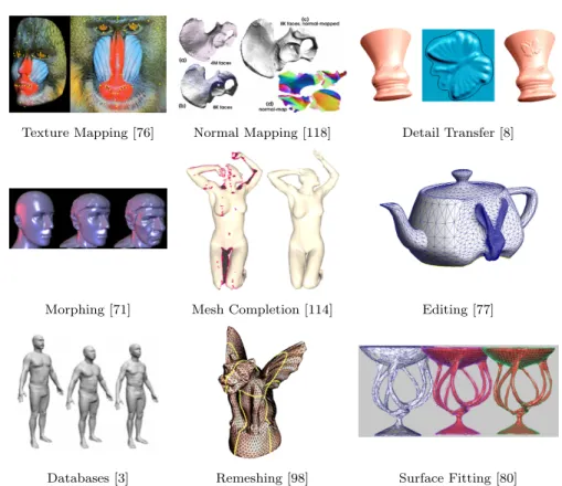
Surface parameterization was introduced to computer graphics as a method for mapping textures onto surfaces [7,84]. Over the last decade, it has gradually become a ubiquitous tool, useful for many mesh pro-cessing applications, discussed below (Figure 1.1).

Detail Mapping Detailed objects can be efficiently represented by a coarse geometric shape (polygonal mesh or subdivision surface) with the details corresponding to each triangle stored in a separate 2D array. In traditional texture mapping, the detail is the local albedo of a Lam-bertian surface. Texture maps alone can enrich the appearance of a surface in a static picture, but since neighboring pixels will have sim-ilar shadowing, objects may still look flat in animations with varying lighting conditions. Bump mapping stores small deviations of the point-wise normal from that of the smooth underlying surface and uses the perturbed version during shading [13]. Normal mapping [118, 130] is a similar technique that replaces the normals directly rather than storing a perturbation. As the light direction changes, the shading variations produced by the normal perturbations simulate the shadows caused by small pits and dimples in the surface. Since the actual geometry of the object is not modified, the silhouettes still look polygonal or smooth. Displacement mapping addresses this problem by storing small local deformations of the surface, typically in the direction of the normal.

1.1. Applications 107

Texture Mapping [76] Normal Mapping [118] Detail Transfer [8]

Morphing [71] Mesh Completion [114] Editing [77]

Databases [3] Remeshing [98] Surface Fitting [80] Fig. 1.1 Parameterization applications.

Recent techniques [75,93,96] model a thick region of space in the neigh-borhood of the surface by using a volumetric texture, rather than a 2D one. Such techniques are needed in order to model detail with compli-cated topology or detail that cannot be easily approximated locally by a height field, such as sparsely interwoven structures or animal fur. The natural way to map details to surfaces is using planar parameterization (Section 3).

Detail Synthesis While the goal of texture mapping is torepresent

the complicated appearance of 3D objects, several methods make use of mesh parameterization tocreatethe local detail necessary for a rich appearance. Such techniques can use as input flat patches with sample detail [92, 97, 119, 127, 129, 131]; parametric or procedural models; or

direct user input and editing [17, 57]. The type of detail can be quite varied and the intermediate representations used to create it parallel the final representations used to store it.

Morphing and Detail Transfer A map between the surfaces of two objects allows the transfer of detail from one object to another [81, 99, 121], or the interpolation between the shape and appearance of several objects [2, 63, 66, 71, 109]. By varying the interpolation ratios over time, one can produce morphing animations. In spatially varying and frequency-varying morphs, the rate of change can be different for different parts of the objects, or different frequency bands (coarseness of the features being transformed) [63,66,71]. Such a map can either be computed directly or, as more commonly done, computed by mapping both object surfaces to a common domain (Sections 5 and 6).

In addition to transferring the static appearance of surfaces, inter-surface parameterizations allow the transfer of animation data between shapes, either by transferring the local surface influence from bones of an animation rig, or by directly transferring the local affine transfor-mation of each triangle in the mesh [122].

Mesh Completion Meshes from range scans often contain holes and multiple components. L´evy [77] uses planar parameterization to obtain the natural shape for hole boundaries and to triangulate those. In many cases, prior knowledge about the overall shape of the scanned models exists. For instance, for human scans, templates of a generic human shape are readily available. Allenet al. [3], and Anguelovet al.[6] use this prior knowledge to facilitate completion of scans by computing a mapping between the scan and a template human model. Kraevoy and Sheffer [67] develop a more generic and robust template-based approach for completion of any type of scans. The techniques typically use an inter-surface parameterization between the template and the scan (Sec-tions 5 and 6).

Mesh Editing Editing operations often benefit from a local parame-terization between pairs of models. Biermannet al.[8] use local parame-terization to facilitate cut-and-paste transfer of details between models.

1.1. Applications 109 They locally parameterize the regions of interest on the two models in 2D and overlap the two parameterizations. They use the parameteriza-tion to transfer shape properties from one model to the other. Sorkine

et al.[121] and L´evy [77] use local parameterization for mesh composi-tion in a similar manner. They compute an overlapping planar param-eterization of the regions near the composition boundary on the input models and use it to extract and smoothly blend shape information from the two models.

Creation of Object Databases Once a large number of models are parameterized on a common domain (Sections 5 and 6), one can perform an analysis determining the common factors between objects and their distinguishing traits. For example on a database of human shapes [3], the distinguishing traits may be gender, height, and weight, while a database of human faces may add facial expressions [10–12, 85]. Objects can be compared against the database and scored against each of these dimensions, and the database can be used to create new plausible object instances by interpolation or extrapolation of existing ones.

Remeshing There are many possible triangulations that represent the same shape with similar levels of accuracy. Some triangulation may be more desirable than others for different applications. For example, for numerical simulations on surfaces, triangles with a good aspect ratio (that are not too small or too “skinny”) are important for convergence and numerical accuracy. One common way to remesh surfaces, or to replace one triangulation by another, is to parameterize the surface, then map a desirable, well-understood, and easy to create triangu-lation of the domain back to the original surface. For example, Gu

et al.[41] use a regular grid sampling of a planar square domain, while subdivision based methods [49, 63, 72] use regular subdivision (usually one-to-four triangle splits) on the faces of a simplicial domain. Such locally regular meshes can usually support the creation of smooth sur-faces as the limit process of applying subdivision rules. To generate high quality triangulations Desbrun et al. [26] parameterize the input mesh in the plane and then use planar Delaunay triangulation to obtain

a high quality remeshing of the surface. One problem these methods face is the appearance of visible discontinuities along the cuts created to facilitate the parameterization.

Surazhsky and Gotsman [123] avoid global parameterization, and instead use local parameterization to move vertices along the mesh as part of an explicit remeshing scheme. Ray et al. [102] use global periodic parameterization to generate a predominantly quadrilateral mesh directly on the 3D surface. Donget al.[26] use a parameterization induced by the Morse complex to generate a quad only mesh of the surface.

More details on the use of parameterization for remeshing can be found in a recent survey by Alliezet al. [5].

Mesh Compression Mesh compression is used to compactly store or transmit geometric models [4]. As with other data, compression rates are inversely proportional to the data entropy. Thus higher compres-sion rates can be obtained when models are represented by meshes that are as regular as possible, both topologically and geometrically. Topo-logical regularity refers to meshes where almost all vertices have the same degree. Geometric regularity implies that triangles are similar to each other in terms of shape and size, and vertices are close to the centroid of their neighbors. Such meshes can be obtained by parame-terizing the original objects and then remeshing with regular sampling patterns [41, 52]. The quality of the parameterization directly impacts the compression efficiency.

Surface Fitting One of the earlier applications of mesh parameteri-zation is surface fitting [32,51,54,80,82]. Many applications in geometry processing require a smooth analytical surface to be constructed from an input mesh. A parameterization of the mesh over a base domain sig-nificantly simplifies this task. Earlier methods either parameterized the entire mesh in the plane [32] or segmented it and parameterized each patch independently (Sections 3 and 4). More recent methods [51,80,82] focus on constructing smooth global parameterizations (Section 5.1) and use those for fitting, achieving global continuity of the constructed surfaces.

1.1. Applications 111

Modeling from Material Sheets While computer graphics focuses on virtual models, geometry processing has numerous real-world engi-neering applications. Particularly, planar mesh parameterization is an important tool when modeling 3D objects from sheets of material, rang-ing from garment modelrang-ing to metal formrang-ing or forgrang-ing [7, 60, 86, 88]. All of these applications require the computation of planar patterns to form the desired 3D shapes. Typically, models are first segmented into nearly developable charts (Section 4), and these charts are then parameterized in the plane (Section 3).

Medical Visualization Complex geometric structures are often bet-ter visualized and analyzed by mapping the surface normal-map, color, and other properties to a simpler, canonical domain. One of the struc-tures for which such mapping is particularly useful is the human brain [42,50,56]. Most methods for brain mapping use the fact that the brain has genus zero, and visualize it through spherical [42, 50] (Section 5.2) or planar [56] (Section 3) parameterization.

Given the vast range of processing techniques that have benefited from parameterization, we expect that many more applications can utilize it as a powerful processing tool.

2

Terminology

Before proceeding to describe various parameterization techniques in the next section, we first briefly establish some terminology. We are concerned with the parameterization of triangle meshes. The topology of such meshes is typically represented as a simplicial complex: a set of 1-, 2-, and 3-element subsets of a set V of labels, corresponding respec-tively to the vertices, edges, and triangles of the mesh. The geometry of the mesh is represented as 3D coordinates associated with each of the vertices c:V → R3, making edges correspond to (open) line segments in 3D, and mesh triangles to (open) triangles in 3D.

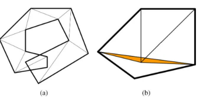
The purpose of mesh parameterization is to obtain a map between such a mesh and a triangulation of a domain. The map is piecewise linear, associating each triangle of the original mesh with a triangle in the domain. An important goal of parameterization is to obtain bijec-tive(invertible) maps, where each point on the domain corresponds to exactly one point of the mesh. Many applications of planar parame-terization can, with some modifications, handle global domain overlaps (Figure 2.1(a)). For such applications the bijectivity requirement can be weakened, requiring only local rather than global bijectivity. Local bijectivity [118] requires a map of any sufficiently small region of the

113

Fig. 2.1 Non-bijective parameterizations: (a) planar embedding with a global overlap; (b) planar embedding with a local overlap. The normal of the highlighted flipped trian-gle is inverted with respect to the other triantrian-gle normals.

mesh to be bijective. This condition is violated when the mappings of adjacent mesh triangles intersect, in this case the parameterization is said to “fold over” or contain “triangle flips” (Figure 2.1(b)).

The geometric shape of the domain triangles will typically be slightly different than the shape of the original triangles, resulting in angle and area distortion. Applications typically try to minimize the distortion for the whole mesh in a least squares sense. Very few meshes admitisometric,namely zero distortion, parameterizations. For exam-ple, only developable surfaces (such as cylindrical or conical sheets) admit planar isometric parameterizations. Maps that minimize the angular distortion, orshear, are called conformal, and maps that min-imize area distortion are called authalic. Often conformal maps are also calledharmonic, though, as shown by Floater and Hormann [35], the two are not equivalent. These terms are borrowed from differen-tial geometry of smooth surfaces, where Riemann’s theorem guaran-tees that conformal maps (with zero angular distortion) always exist, mapping any infinitesimally small circle on the surface to a circle on the domain, and thus preserving angles, but allowing the scale factor of the transformation to vary across the map. The Riemann theorem does not hold for meshes. For instance, when considering planar parameter-ization, the sum of angles around an interior mesh vertex in 3D can vary, while the sum of angles around a vertex in the plane is always 2π. Some conformal parameterization methods applied to a series of pro-gressively denser meshes of the same object (with smaller and smaller

triangles, obtained through subdivision) will converge in the limit to a smooth conformal map. The conformality of a mesh can be measured in multiple different ways [25,54,79,113], resulting in different function-als to be optimized. For instance, Hormann and Greiner [54] consider

the minimal and maximal eigenvaluesγ and Γ of the first fundamental

form of the mapping. Alternatively, Sheffer and de Sturler [113] directly measure the difference between the corresponding angles in the mesh and domain triangles.

As pointed out by Floater and Hormann [34], though authalic parameterizations are achievable, they are not very useful by them-selves, as they allow extreme angular and linear distortion. Thus, meth-ods that consider area preservation [24, 25] typically balance it with angle preservation.

Other metrics of parameterization distortion measure the preserva-tion of distances across the mesh [107, 138, 140]. The stretch metrics

proposed by Sander et al.[107] are now commonly used in the

graph-ics community as standard measures of distance preservation. Sander

et al.[107] observe that the linear map over each triangle can be decom-posed into a translation, a rotation, and a non-uniform scale along two orthogonal axes. The two scale factors 0≤γ≤Γ are the singular val-ues of the transformation matrix, or the square roots of the eigenvalval-ues of the integrated metric tensor (the transpose of the matrix times the matrix itself). Intuitively, the linear transformation map will stretch a unit circle to an ellipse with axes γ and Γ. The L_∞ stretch for a triangle is defined by Sanderet al.[107] as max(γ,Γ) = Γ, while the L2

stretch is defined as (γ2_{+ Γ}2_{)/2. The name for the stretch metric}

comes from applications that map signals with regular sampling in the domain to 3D surfaces; these applications want to minimize the stretch of the signal over the surface, or the space between the locations of mapped samples. In other words, stretch penalizes undersampling the mesh, but not oversampling it.

When parameterizations are used to resample or compress 3D objects, the quality of the reconstruction can be measured by the sym-metric Hausdorff sym-metric between the original and reconstructed meshes. This metric measures the maximum distance between any point on either mesh and its projection on the other mesh. In practice most

115 people use an RMS-average of these point distances. For compression schemes that allow trade-offs between the bit rate (file size) and approx-imation accuracy, the performance is measured using rate-distortion curves, plotting one against the other.

Keeping these definitions in mind, we now proceed to survey the parameterization techniques available.

3

Parameterization of Topological Disks

The early papers to address parameterization for computer graph-ics applications were interested in planar parameterization of meshes with disk-like topology. The first application for such parameteriza-tions was texture mapping. More recent applicaparameteriza-tions include map-ping of other surface properties such as normals or BRDFs, and mesh processing operations such as remeshing and compression. Two recent surveys [34, 35] list more than 20 different planar parameteri-zation techniques. Both surveys focus on the mathematical aspects of these techniques. To avoid unnecessary overlaps, we will address the more practical considerations, such as the suitability of the techniques for computer graphics applications in terms of distortion (type and amount), robustness, and efficiency. In our discussion, we classify the methods based on the type of parametric distortion minimized.

Planar parameterization of 3D surfaces inevitably creates distortion in all but special cases. A well-known result from differential geometry is that for a general surface patch there is no distance-preserving (iso-metric) parameterization in the plane [26]. Distance-preserving param-eterizations exist only for developable surfaces: that is, surfaces with

117 zero Gaussian curvature. Cutting the surface into charts or introducing seams (as discussed in Section 4), can reduce this distortion.

We classify planar parameterizations into roughly four groups: methods that ignore distortion altogether (Section 3.1), methods that minimize angular distortion (Section 3.2), methods that minimize stretch (Section 3.3), and methods that minimize area distortion (Section 3.4). There are also several techniques providing tools for achieving a trade-off between different types of distortion (Section 3.5). Ideally, most parameterization applications work best on zero dis-tortion parameterizations, though most are tolerant to some amount of distortion, some being more tolerant to shear and others to stretch. In general, applications that depend on regular grids for sampling, such as different types of detail mapping and synthesis, as well as compression and regular resampling schemes (e.g., geometry images [41]), tend to perform better on stretch minimizing parameterizations, since stretch is directly related to under-sampling. In contrast, applications based on irregular sampling, such as remeshing [25], are very sensitive to shear-ing, but can handle quite significant stretch. When acceptable levels of shear or stretch are not attainable because a surface is too complex, the surface needs to be cut prior to parameterization (Section 4) in order to achieve acceptable distortion.

In addition to distortion, several other factors should be considered when choosing a parameterization method for an application at hand:

• Free versus fixed boundary Many methods assume the boundary of the planar domain is pre-defined and convex. Fixed-boundary methods typically use very simple formula-tions and are very fast. Such methods are well suited for some applications, for instance those that utilize a base mesh parameterization, see Section 5.1. Free-boundary tech-niques, which determine the boundary as part of the solu-tion, are often slower, but typically introduce significantly less distortion.

• Robustness Most applications of parameterization require it to be bijective. For some applications local bijectivity (no triangle flips) is sufficient, while others require global

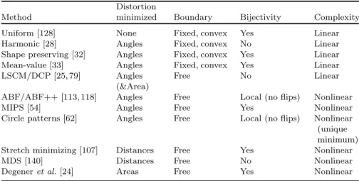
Table 3.1 Planar method summary. Distortion

Method minimized Boundary Bijectivity Complexity Uniform [128] None Fixed, convex Yes Linear Harmonic [28] Angles Fixed, convex No Linear Shape preserving [32] Angles Fixed, convex Yes Linear Mean-value [33] Angles Fixed, convex Yes Linear LSCM/DCP [25, 79] Angles

(&Area)

Free No Linear

ABF/ABF++ [113, 118] Angles Free Local (no flips) Nonlinear

MIPS [54] Angles Free Yes Nonlinear

Circle patterns [62] Angles Free Local (no flips) Nonlinear (unique minimum) Stretch minimizing [107] Distances Free Yes Nonlinear

MDS [140] Distances Free No Nonlinear

Degeneret al.[24] Areas Free Yes Nonlinear

bijectivity conditions (the boundary does not self-intersect). Only a subset of the parameterization methods can guarantee local or global bijectivity. Some of the others can guarantee bijectivity if the input meshes satisfy specific conditions.

• Numerical Complexity The existing methods can be roughly classified according to the optimization mechanism they use into linear and nonlinear methods. Linear methods are typically significantly faster and simpler to implement. However, as expected the simplicity usually comes at the cost of increased distortion.

Table 3.1 provides a summary of a number of popular recent meth-ods with respect to these four criteria. Figures 3.1–3.4 and Table 3.2 provide distortion and runtime comparison between some of the more popular recent methods.

3.1 Planar Mesh Embedding

One of the oldest methods referenced in the context of mesh parameter-ization is the graph embedding method of Tutte [128]. Tutte’s formu-lation of graph embedding directly applies to triangular meshes. It also

3.1. Planar Mesh Embedding 119

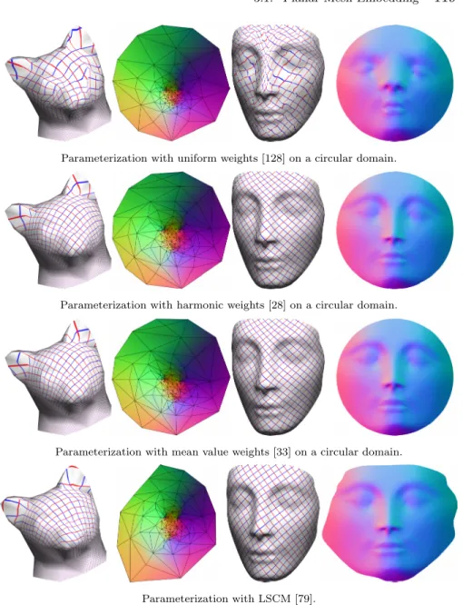
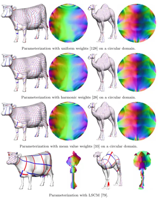
Parameterization with uniform weights [128] on a circular domain.

Parameterization with harmonic weights [28] on a circular domain.

Parameterization with mean value weights [33] on a circular domain.

Parameterization with LSCM [79]. Fig. 3.1 Linear parameterization methods.

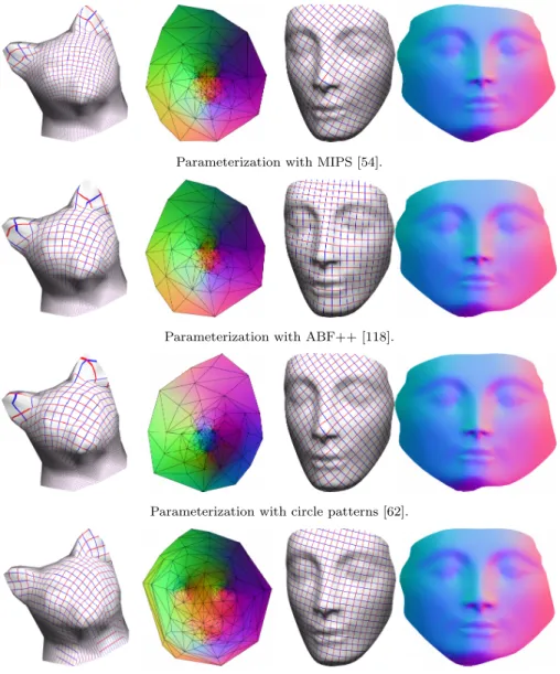
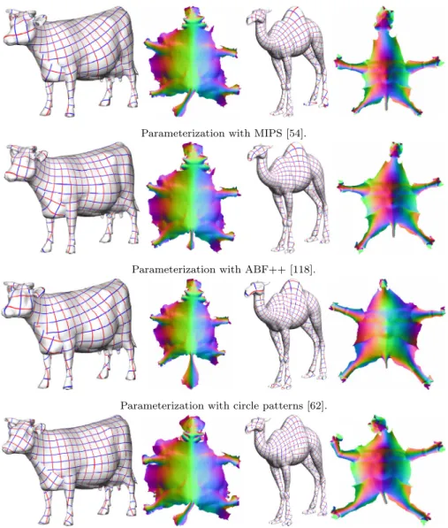
Parameterization with MIPS [54].

Parameterization with ABF++ [118].

Parameterization with circle patterns [62].

Stretch minimizing parameterization [107]. Fig. 3.2 Nonlinear parameterization methods.

provides a general framework employed by many more-recent methods. The graph embedding formulation uses a two stage procedure. First, the boundary vertices of the mesh are mapped to the boundary of a convex region in 2D. Then the positions of the rest of the vertices are

3.1. Planar Mesh Embedding 121

Parameterization with uniform weights [128] on a circular domain.

Parameterization with harmonic weights [28] on a circular domain.

Parameterization with mean value weights [33] on a circular domain.

Parameterization with LSCM [79].

Fig. 3.3 Linear parameterization methods on closed objects with a seam.

obtained by solving a linear system of the form Lu= 0, Lv= 0

L_i,j =

  

−_k=iLi,k i=j

w_ij (i, j)∈E

0 otherwise

Parameterization with MIPS [54].

Parameterization with ABF++ [118].

Parameterization with circle patterns [62].

Stretch minimizing parameterization [107]. Fig. 3.4 Nonlinear parameterization for closed objects with a seam.

The system is solved independently for the u and v coordinates.

The parameter values of the fixed boundary vertices are used to specify the boundary conditions for the system. The weights w_ij are defined for each edge of the mesh. It was proven [32, 128], that if the weights are positive and the matrix is symmetric, then the obtained

3.2. Angle-Preserving Parameterization 123 parameterization is guaranteed to be bijective. Tutte [128] used uniform unit weights, settingw_ij = 1 iff (i, j) is an edge in the mesh. Note that this setting definesLas the classical graph Laplacian matrix [19]. While the resulting parameterization is provably bijective, it does not preserve any shape properties of the mesh (Figures 3.1 and 3.3, top row).

Another well known, but less frequently used, mesh embedding tech-nique is based on the circle packing theorem [104]. Given a triangular mesh, a circle packing is a collection of circles, one for each mesh ver-tex, such that two circles are tangential if there is a mesh edge between their associated vertices. By connecting the centers of these circles we obtain a planar embedding. The circle packing theorem states that for any given triangular mesh with disk topology and for any selection of radiirassociated with the boundary vertices of the mesh, there exists a unique (up to symmetries) circle packing of the mesh with boundary cir-cles having these radii. Collins and Stephenson [23] provide a construc-tive technique to use the theorem to obtain mesh embeddings based only on combinatorial mesh information. Thus the method is guar-anteed to generate bijective embeddings but does not preserve shape properties.

3.2 Angle-Preserving Parameterization

Many of the disk-parameterization methods are focused on minimizing the angular distortion, or shear, of the parameterization. Several appli-cations require angle-preserving parameterization; for instance, remesh-ing replaces one triangulation with another of better quality, typically by mapping a regular triangulation of the domain onto the mesh. The quality is often defined in terms of angles: numerical simulations are adversely affected by small angles, while good compression depends on regular structures with triangles similar to their neighbors.

Angle-preserving parameterizations are efficient to obtain and are also often suitable for other applications, such as texture mapping, as long as the stretch of the parameterization is relatively low. This is often the case when the parameterized surfaces are not too far from developable. Riemann’s theorem [26] states that for smooth surfaces a conformal planar parameterization exists for any planar domain. Thus,

since meshes are often viewed as approximations of smooth surfaces, we can argue that it is possible to map them to the plane with very little angular distortion.

Several parameterization techniques [28,32,33] use an approach sim-ilar to Tutte’s [128]. They first map the boundary of the surface to the boundary of a convex domain in 2D and then obtain the param-eterization for the rest of the vertices solving a system of equations (Equation (3.1)), independently for theu andvcoordinates. The main difference between these methods is in the valuesw_ij assigned as edge weights. The choice of weights influences both the distortion and the bijectivity of the parameterization.

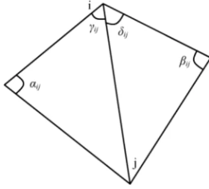
The harmonic or cotangent weights [28, 94] are perhaps the most widely known in the graphics community. They define the matrix ele-ments as:

w_ij = (cotα_ij + cotβ_ij)/2, (3.2)

whereα_ij andβ_ij are the opposite angles in the two triangles shared by the edge (i, j) as shown in Figure 3.5. These weights are derived from a finite-element description of harmonic energy and therefore aim at reducing the angular distortion of the parameterization. The greatest drawback of harmonic parameterization is that if the mesh contains obtuse angles, the weights can be negative, and, as a result, the param-eterization can be non-bijective. Hence this formulation is not suit-able, as is, for applications where bijectivity is a major concern. In

3.2. Angle-Preserving Parameterization 125 practice many methods suggest first improving the mesh quality by bisecting obtuse angles or flipping edges. It has been proven that if the mesh satisfies the Delaunay criterion, even if it contains obtuse triangles, the parameterization obtained using the cotangent weights (Equation (3.2)) will always be bijective. Recently, Kharevychet al.[62] suggested using an “intrinsic” Delaunay triangulation of the surface as an input to the harmonic mapping to guarantee bijectivity. Figures 3.1 and 3.3 show a few examples of parameterizations generated using har-monic parameterization on a circular domain.

The shape-preserving parameterization [32] is also based on discrete harmonic mapping. It uses weights which are positive and symmetric thus ensuring that the parameterization is always bijective. However, the weights vary non-smoothly, i.e., they have derivative discontinu-ities, as the vertex i moves inside its one-ring polygon. Guskov [47] modifies the shape preserving parameterization [32] by introducing an extra term that allows an anisotropic parameterization stretched in the direction of a given surface direction field.

The mean-value weights also proposed by Floater [33] are much simpler and vary smoothly

w_ij = (tan(γ_ij/2) + tan(δ_ij/2))/c(i)−c(j),

where c(i) and c(j) are the 3D positions of vertices i and j, and γ_ij and δ_ij are the angles in the two triangles shared by the edge (i, j) shown in Figure 3.5. The mean-value weights are always positive. The resulting matrix is not symmetric (w_ij =w_ji) thus the bijectivity proof of Tutte [128] does not directly apply to this formulation. Neverthe-less, Floater [33] proves that mean-value parameterization is guaran-teed to be bijective. As shown in Figures 3.1 and 3.3 (third row) the mean-value weights lead to parameterizations with small angular dis-tortion. However, it was demonstrated [135] that they can in some cases introduce larger angular distortion than the more commonly used har-monic weights [28].

All of these techniques are very efficient and simple to implement as they only require solving a single linear system. However, since the parameterization distortion depends on how close the actual boundary shape matches the 2D domain shape, the fixed-boundary techniques

perform poorly when the 3D meshes have non-convex boundaries (Figure 3.3), or boundaries that differ significantly from the specified boundary of the planar domain. Thus, these techniques work best when the inputs have well-shaped nearly convex boundaries. For instance, in a base-mesh setting (Section 5.1) the input mesh is first segmented into nearly triangular patches. In this setting, the fixed-boundary methods introduce very little distortion when mapping the patches to the cor-responding triangular base mesh faces.

To reduce the distortion, the boundary of the 2D domain can be computed as part of the solution. Leeet al.[74] free the domain bound-ary by introducing one or more layers of triangles around the original boundary in 3D, creating a virtualboundary (Figure 3.6(a)). The vir-tual boundary is fixed onto a given convex polygon and the mapping for the rest of the vertices is computed using Floater’s method [32]. Since the original boundary vertices are free to move, the method obtains a parameterization with less distortion than with the original convex combination approach (Figure 3.6). A similar idea was used by Kos and Varady [65]. Zhanget al. [137] usescaffold triangles in the virtual boundary that only contribute a flip penalty to a stretch-like optimiza-tion metric.

Recently, two explicit formulations of free-boundary, linear param-eterization, LSCM and DCP, were independently proposed by

Fig. 3.6 (a) Adding a virtual boundary to the original mesh. (b) Shape Preserving [32] parameterization of the original mesh. (c) Parameterization of the original mesh and its virtual boundary [74]. The virtual boundary vertices are fixed, allowing the real boundary vertices to move.

3.2. Angle-Preserving Parameterization 127

Fig. 3.7 LSCM [79] notations.

L´evy et al. [79] and Desbrun et al. [25]. Using different formulations of harmonic energy, both sets of authors derived equivalent formula-tions for free-boundary parameterization that aim to minimize angular distortion. The formulation of L´evyet al.[79] is based on the observa-tion that given the anglesα1,α2,α3 of a planar triangle (Figure 3.7)

the following holds:

(u3, v3)−(u1, v1) =

sinα2

sinα3

Rα1_[(u

2, v2)−(u1, v1)], (3.3)

whereu_i, v_i are the planar coordinates of the triangle vertices andRα

a rotation matrix with angle α. To minimize angular distortion the

authors plug the original 3D angles into the formula and minimize the sum of square distances between the left and right sides of Equa-tion (3.3). They fix two vertices to avoid the degenerate soluEqua-tion where all the vertices are at one point. Interestingly, the conditions speci-fied by these two methods for interior mesh vertices are equivalent to the discrete harmonic energy formulation (Equation (3.2)). Thus the difference in the results can be viewed as a difference in the imposed boundary conditions.

Figures 3.1 and 3.3 (bottom row) show some models parameter-ized with LSCM. As demonstrated LSCM/DCP introduce significantly less distortion than fixed boundary approaches, particularly near the domain boundaries. The methods do not guarantee local or global bijec-tivity, and can theoretically result in both flipped triangles and global

overlaps. The HLSCM method [101] describes a mechanism for speed-ing up the solution process for LSCM usspeed-ing a hierarchical solver.

On meshes with high curvature, nonlinear conformal methods, dis-cussed below, introduce significantly less stretch than DCP/LSCM (Figure 3.4). The MIPS method [54, 55] optimizes a nonlinear func-tional that measures mesh conformality (Figures 3.2 and 3.4, top row). To obtain a solution it starts with a harmonic fixed-boundary parame-terization [32] as an initial guess. It then proceeds to move vertices one at a time to reduce the distortion metric. To prevent flips, vertices are only permitted to move inside the kernel of neighboring vertices. When moving boundary vertices, the method also checks for boundary over-laps and prevents those. Thus, it guarantees that the resulting param-eterization remains globally bijective throughout the procedure. The authors advocate the use of conformal mapping for remeshing [69] and surface fitting [53].

Instead of defining a planar parameterization in terms of vertex coordinates, the ABF method [113,114] defines it in terms of the angles of the planar triangles. Sheffer and de Sturler [113] specify a set of con-straints that angle values have to satisfy to define a planar triangular mesh. They search for angles that are as close as possible to the original 3D mesh angles and that satisfy those constraints. They then convert the solution angles into actual (u, v) vertex coordinates. The resulting parameterizations are guaranteed to have no flipped triangles (local bijectivity) but can contain global overlaps. The authors provided a mechanism for resolving such overlaps, but it has no guarantees of con-vergence. The original ABF method is relatively slow and suffers from stability problems in the angle-to-uvconversion stage for large meshes. ABF was augmented to yield ABF++ [118], a technique addressing both problems (Figures 3.2 and 3.4, second row). ABF++ introduces a stable angle-to-uv conversion and drastically speeds up the solution by introducing both direct and hierarchical solution approaches.

Zayeret al. [133] proposed to extend ABF by using additional straints on the angles enforcing the parameter domain to have con-vex boundaries, thus guaranteeing global bijectivity. Zayer et al.[135] introduce an iterative free-boundary conformal method. They start with a fixed-boundary parameterization and then relax it. In their

3.2. Angle-Preserving Parameterization 129

Fig. 3.8 Setting the boundary free [135].

comparisons, the method seems to be faster but introduce more distor-tion than ABF and MIPS (Figure 3.8).

Hurdal et al. [56] and Bowers and Hurdal [15] compute

angle-preserving parameterizations using a variation of the circle-packing for-mulation described later by Collins and Stephenson [23]. They observe that, in the circle-packing setting, angle preservation corresponds to preservation of specified distances between circles. They construct pat-terns of non-intersecting circles, where each circle corresponds to a vertex of a triangulation. To preserve angles, they optimize distances between circles corresponding to neighboring vertices. The authors use the conformal mapping technique for medical visualization, focusing on visualizing the structure of the human brain.

Kharevych et al. [62] use a circle patterns approach where each

circle corresponds to a mesh face. In contrast to classical circle pack-ing, they use intersecting circles, with prescribed intersection angles. Given these angles, the circle radii follow as the unique minimizer of a convex energy. The method first computes the intersection angles using nonlinear constrained optimization and then finds the energy minimizer. Since the solution for the intersection angles is conformal only for a Delaunay triangulation, the authors employ a pre-processing stage that involves “intrinsic” Delaunay triangulation. At the final stage of the method, the computed angles are converted to actualuv -coordinates. The method supports equality and inequality constraints on the angles along the boundary of the planar parameter domain. Similar to ABF, the parameterization is locally bijective, but can con-tain global overlaps. As shown in Figures 3.2 and 3.4, the amount of

Table 3.2 Timings (s) of various parameterization techniques. Method Cat head (257 ∆) Nefertiti (8071 ∆) Cow (5804 ∆) Camel (78K ∆)

Uniform [122]* 0.02 0.23 0.14 2.91

Harmonic [28]* 0.02 0.26 0.17 3.21

Mean-value [33]* 0.02 0.25 0.16 3.19

LSCM [79]* 0.03 0.38 0.20 5.28

ABF++ [118]* 0.06 1.87 0.77 36.31

MIPS [54]‡ 1 8 5 83

Circle patterns [62]* 0.1 3.6 2.1 76.7 Stretch minimizing [107] 5.17† 12 8.5 127

†_{1.2 GHz Pentium M;}∗_{3.0 GHz Pentium 4;}‡_{3.2 GHz Pentium 4.}

distortion introduced by the method is comparable with that of other nonlinear conformal techniques. Kharevychet al.propose an extension of the method to global parameterization of meshes by introducingcone singularites, as described in Section 6.

Karniet al. [61] propose an interesting iterative method for resolv-ing triangle flips in existresolv-ing planar triangulations. The input to their method is a planar triangulation generated by one of the methods above. If the triangulation contains flipped triangles they employ an iterative vertex relocation procedure to eliminate the flips. Their method can also be used to support soft positional constraints in pla-nar triangulations. The method reduces the number of flipped triangles does not guarantee that the final triangulation will be flip-free.

Table 3.2 lists the runtimes for the different conformal methods. We used the Graphite 3D modeling system [39] to time the fixed-boundary methods, LSCM and ABF++. For the other methods the timings were provided by the authors. As expected, linear techniques are about one order of magnitude faster than the nonlinear ones. Nevertheless, even the nonlinear methods are fairly fast taking less than two minutes to process average size models.

3.3 Distance Preserving Parameterization

In contrast to conformal parameterization, which always exists for smooth surfaces, stretch- or distance-preserving parameterization exists only for developable surfaces. Hence existing methods aim at

3.3. Distance Preserving Parameterization 131 minimizing linear distortion rather than completely eliminating it. Early parameterization techniques [7, 78, 84] introduced distance min-imizing formulations which were numerically quite complex and thus hard to minimize.

Sanderet al.[107] introduce two metrics of parameterization stretch (L2 andL∞), described in Section 2. These two stretch metrics are now

commonly used for comparing linear distortion between parameteriza-tions [62, 118, 138]. They then proceed to minimize theL2 metric using

a solution mechanism similar to that of Hormann and Greiner [54], starting with a shape-preserving parameterization [32] and moving one vertex at a time (Figures 3.2 and 3.4, bottom row). To speed up the parameterization, the authors use a hierarchical top-down parameter-ization approach. Similar to MIPS, the stretch minimparameter-ization method starts with non-self-intersecting parameter domains, therefore, it can effectively prevent both flips and global overlaps, thus guaranteeing globally bijective parameterization. Since the method’s goal is to mini-mize anL2 norm, it sometimes compensates for shrinkage in one

direc-tion by stretching in another, introducing shearing (see camel’s neck in Figure 3.4, bottom row). Example runtimes for the method are listed in Table 3.2. The runtimes are slower but within the same order of mag-nitude as those of the nonlinear conformal methods. Sanderet al.[106] introduced an extension of the method to signal specialized parameter-ization, where the user can influence the distribution of the distortion across the surface. This method assumes that the reconstructed signal is piecewise constant. Tewariet al.[125] assume that the reconstruction is piecewise linear, which provides greater sensitivity to signal detail.

Zigelman et al. [140] introduce a mesh parameterization method

that aims to preserve the distances between all pairs of vertices on the surface. They first compute those distance using geodesics, and then use multi-dimensional scaling (MDS) to embed the mesh in the plane. The method performs quite well for surfaces that are close to developable. However, for complex surfaces, it often tends to fold the surface in the plane generating a non-bijective parameterization, since the folded solution provides better distance preservation [138].

Zhouet al.[138] also use an MDS orisomapbased approach, intro-ducing several mechanisms to speedup the computation process. If the

parameterized planar mesh contains folds, they segment the surface, and parameterize each chart independently (Section 4). Figure 3.9(b) shows the charts and the parameterization produced by the method.

In some settings it is possible to avoid solving a linear system and simply compute the parameterization one triangle at a time [86, 120]. However, for most meshes this technique must be combined with simul-taneous generation of cuts in the mesh surface. We therefore choose to discuss it together with other cutting techniques in Section 4.

3.4 Area-Preserving Parameterization

As pointed out by Floater and Hormann [35], from a theoretical point of view, there are two independent qualities that can be minimized in a mapping: angular distortion and area distortion. For continuous sur-faces, whereas conformal mappings are nearly unique, area-preserving

mappings are not. Thus methods that search for authalic, namely

area-preserving, mesh parameterizations typically introduce additional optimization terms or constraints on the parameterization. Desbrun

et al. [25] use a similar derivation of their conformal DCP embed-ding to obtain a linear formulation for local area preservation. Degener

et al. [24] develop a nonlinear formulation of per-triangle area preser-vation. Both papers then proceed to combine the area optimization metric with a conformality metric to allow for parameterizations that mediate between the two as explained in the next section.

3.5 Trade-Off Between Metrics

Many applications of parameterizations fail when either the shear or the stretch are extreme. However, they can tolerate a small amount of either type of distortion. Thus it is sometimes advisable to provide a parameterization that provides an adequate degree of trade-off between angle preservation and area, or length preservation.

Desbrun et al. [25] provide a linear formulation which supports a trade-off between angular and area distortion. It is not clear if the combined formulation can be used in a free-boundary setting. Degener

3.5. Trade-Off Between Metrics 133

Fig. 3.9 Segmentation and texture atlases for (a) Isocharts [138] – 13 charts; (b) L´evy

et al.[79] – 44 charts; (c) D-charts [60] – 12 charts; (d) multi-chart geometry images [108] – 15 charts; and (e) Zhanget al.[137] – 24 charts.

that mediate between angle and area deformation by modifying the minimized functional. They define the minimized energy to be a sum of per-triangle terms. Each term is a product of the MIPS harmonic energy per-triangle and an energy functional that measures area distor-tion. The powers of the components in the product provide the media-tion between the two measures. The method maintains the bijectivity guarantees of the original MIPS algorithm. Clarenzet al.[20] provide a different set of nonlinear energy metrics allowing for trade-off between angle, area, and distance distortion measures.

In recent years, a number of researchers suggested using a two stage approach. First, a mesh is parameterized using one of the existing tech-niques listed above, and then a second, post-processing stage is applied to improve the parameterization. The improvement typically focuses on reducing some measure of distortion, or providing a trade-off between several distortion measures. The methods measure the distortion of parameterization produced by the first stage of the algorithm, and then adopt the parameters of the second stage to reduce this distortion.

Sheffer and de Sturler [115] first computed an angle-preserving parameterization using ABF [113]; they then used an overlay grid to compute the stretch of the resulting parameterization; finally, they smoothed the overlay grid to mitigate the stretch.

Yoshizawaet al.[132] and Zayeret al.[134] also start with a parame-terization that minimizes angular distortion. They first use linear, fixed-boundary methods to compute one. They then compute the stretch of the parameterization; scale the weights used in the linear method by a mitigating factor and solve the linear system again. To scale the weights, Yoshizawa et al. [132] used the stretch metric of Sander

et al.[107], while Zayeret al.[134] use a simpler construction based on inverse edge lengths.

4

Cutting/Chart Generation

Planar parameterization is only applicable to surfaces with disk topol-ogy. Hence, closed surfaces and surfaces with genus greater than zero have to be cut prior to planar parameterization. As previously noted, greater surface complexity usually increases parameterization distor-tion, independent of the parameterization technique used. To allow parameterizations with low distortion, the surfaces must be cut to reduce the complexity. Since cuts introduce discontinuities into the parameterization, a delicate balance between the conflicting goals of small distortion and short cuts has to be achieved. It is possible to use constrained parameterization techniques to reduce cross-cut disconti-nuities [68, 139] as discussed in Section 6. Cutting and chart generation are most commonly used when computing parameterizations for map-ping of textures and other signals onto the surface. They are also used for applications such as compression [41] and remeshing.

The techniques for cutting surfaces can be roughly divided into two categories: segmentation techniques which partition the surface into mul-tiple charts (Section 4.1), and seam generation techniques which intro-duce cuts into the surface but keep it as a single chart (Section 4.2). Multiple charts created by segmentation typically have longer boundaries

than those created by seam cutting. However, they can often be more effi-ciently packed (Section 4.1.1) into a compact planar domain.

4.1 Mesh Segmentation

Depending on the application, mesh segmentation techniques use differ-ent criteria for creating charts [110]. Segmdiffer-entation techniques, used for parameterization, break the surface into several charts such that the parametric distortion when parameterizing each chart is sufficiently low, while the number of charts remains small and their boundaries are kept as short as possible. Since planes are developable by defini-tion, one possible approach is to segment the surface into nearly planar charts [21, 36, 84, 107, 108].

Earlier approaches are based on incremental clustering of mesh faces into charts. They typically start by selecting several initial seed mesh faces, and then grow the charts around those seeds, adding one mesh face at a time, until all the faces are classified as belonging to one chart or the other.

Recently, Sander et al. [108] introduced a segmentation method

inspired by Lloyd quantization (Figure 3.9(d)). Their algorithm iterates between chart growing and reseeding stages. After each chart growing iteration, the method selects the best seeds with respect to each chart and repeats the process. The authors demonstrate that by iterating, they obtain better results than single pass methods such as that of Sanderet al. [107].

Planes are a special type of developable surfaces. Thus for param-eterization purposes planar segmentation is over-restrictive and usu-ally generates more charts than necessary. Several recent approaches

focused on developable segmentation instead [60, 79, 138]. L´evy

et al.[79] proposed to detect high mean-curvature regions on the mesh and then generate charts starting from seeds which are farthest from those regions (Figure 3.9(b)). This approach tends to capture many developable regions, but can also introduce charts which are far from developable.

Zhou et al. [138] propose a segmentation method based on spec-tral analysis of the surface (Figure 3.9(a)). They compute a matrix of

4.1. Mesh Segmentation 137 geodesic mesh distances and then perform face clustering by growing charts around thenfarthest points in a space defined by the dominant eigenvectors of the matrix.

Zhanget al. [137] use a Reeb graph connecting the critical points of the average geodesic distance to cut the mesh, reducing its genus to zero. The surface is further segmented into features by finding field iso-contours where the feature area increases significantly; then the features are classified as linear ellipsoids, flat ellipsoids, or spheres, and cut using a lengthwise, circular, or, respectively, a “baseball seam” cut. The resulting pieces are close to being developable and can be parameterized with little distortion (Figure 3.9(e)).

Similar to Sanderet al.[108], Julius et al. [60] use Lloyd iterations of growing and reseeding. But instead of looking for planar regions they search for a larger subset of developable surfaces, the so called “devel-opable surfaces of constant slope,” which are characterized by having a constant angle between the normal to the surface and some axis vector. They provide a metric to measure if a chart closely approximates such a surface, and use this metric in the chart growing and reseeding stages (Figure 3.9(c)).

4.1.1 Chart Packing

Chartification techniques raise an additional post-processing challenge. Following the parameterization of each individual chart, those charts

need to be placed, or packed, in a common parameter domain. For

efficient storage of the parameterized meshes, the packing has to be as compact as possible. The optimal packing problem is NP-hard [87], thus only heuristic or approximate packing algorithms exist. The Tetris algorithm [79] introduces charts one by one, searching for the best fit along the active-front of the charts packed so far (Figure 3.9(b)).

Sander et al. [108] extend this algorithm, testing for more options

(Figure 3.9(d)). Zhou et al. [138] use a similar approach but consider also non-square parameter domains (Figure 3.9(a)).

If discontinuities along chart boundaries are not a concern, one way to obtain a parameterization with very low distortion is to view each triangle as a single chart. In this case, the challenge of chartification shifts to finding compact packing [16].

When the shape of the charts is fixed, more efficient packing is pos-sible. Tarini et al. [16] parameterize a 3D mesh over a set of square charts as described in Section 5.1. They then store texture as a collec-tion of small square images, and are able support triangles spanning multiple charts and perform correct filtering across tile boundaries by storing a secondary index structure. Mesh vertices have 3D, rather than 2D, texture coordinates, mapping them to the space in the vicinity of a base domain formed by several cubes glued together. These 3D coor-dinates are interpolated for each pixel drawn for the mesh, and then a fragment program on the graphics card projects them onto a nearby cube face (identified using a small 3D texture) and reads the associated texture for the face.

4.2 Seam Cutting

It is possible to reduce the parameterization distortion without cutting the surface into separate patches by introducing multiple partial cuts or seams inside a single patch. This typically leads to shorter cuts than those created by segmentation. Piponi and Borshukov [95] generated such cuts manually using a network of edges.

McCartney et al.[86] and Sorkine et al.[120] perform parameteri-zation and cutting simultaneously. They unfold the mesh vertices onto the plane one after the other, optimizing the local mapping. Whenever the distortion of the mapping reaches a threshold, Sorkine et al.[120] cut the mesh to reduce it. As a result they have a hard bound on the distortion, but can end up with long and complicated boundaries (Figure 4.1(a)). To measure distortion, Sorkineet al. [120] use the sin-gular valuesγ and Γ of the per-triangle mapping (Section 2).

Gu et al. [41] use parameterization results to facilitate the cut-ting process. The authors first parameterize the surface using shape-preserving parameterization [32]. They then find the point of maximal parametric distortion on the mapping, and generate the shortest cut from the surface boundary to that point. They repeat the process until the distortion falls below a certain threshold (Figure 4.1(b)).

The Seamster algorithm [112, 117] considers the differential geom-etry properties of the surface, independent of a particular parameter-ization technique. It first finds regions of high Gaussian curvature on

4.2. Seam Cutting 139

Fig. 4.1 Generating seams: (a) Sorkineet al.[120]; (b) geometry images [41]; and (c) seam-ster [117]. The color in (c) shows visibility – green is more visible, red is less. The Seamseam-ster cuts go across the palm which is considered more occluded than the back of the hand.

the surface and then uses a minimal spanning tree of the mesh edges to connect those. Finally, it cuts the mesh along the tree edges. While Sheffer [112] uses only the edge length criterion when generating the cuts, Sheffer and Hart [117] use a visibility metric as an edge weight when computing the minimal spanning tree. This way they are able to trace the cuts through the less visible parts of the surface hiding the potential cross-cut discontinuities in texture or other maps on the surface (Figure 4.1(c)). This algorithm was also used to cut the cow and camel in Figures 3.3 and 3.4.

While methods that segment meshes into multiple charts implic-itly generate charts with disk topology, seam cutting methods, such as those of Sheffer and Hart [117] and Gu et al. [41] require an explicit pre-processing stage to convert surfaces with high genus into topological disks. The generation of minimal length cuts that convert a high genus surface into a topological disk is NP-hard [30]. Lazaruset al.[70] intro-duce a method for extraction of canonical schema, converting a high genus surface into a topological disk which in practice produces rela-tively short cuts. Erickson and Har-Peled [30] propose a handle cutting method which has some elegant theoretical guarantees but is complex

to implement. A more practical approach is taken by Gu et al. [41],

who trace a spanning graph of all the faces in the mesh and then prune this graph, obtaining a genus reducing cut. Niet al.[90] smooth scalar functions over a mesh obtaining “fair” Morse functions that have few critical points and whose Morse complexes generate a small number of cuts for genus reduction.

5

Alternate Base Domains

Some applications are quite sensitive to discontinuities in the param-eterization, or cannot tolerate them at all. In such cases, when the object to be parameterized is not a topological disk, it is worthwhile to use a different base domain for the parameterization. Examples of such domains that have been investigated include simplicial complexes (Section 5.1), spheres (Section 5.2), and periodic planar regions with transition curves (Section 5.3).

In addition, numerous applications of parameterization require cross-parameterization or inter-surface mapping between multiple mod-els [66, 109]. Pair-wise mappings between modmod-els can be used for the transfer of different properties between the models, including straight-forward ones, such as texture, and less obvious ones such as deformation and animation [122]. It can also be used for blending and morph-ing [3, 66, 109], as well as mesh completion and repair [67]. The most common approach for pair-wise mapping is to parameterize both mod-els on a common base domain. Free-boundary planar parameterization is clearly unsuitable for this purpose. Instead, alternate domains such as a simplicial complex or a sphere are commonly used.

5.1. Simplicial and Quadrilateral Complexes 141

5.1 Simplicial and Quadrilateral Complexes

Historically, the most popular non-planar base domain has been a sim-plicial complex [48, 49, 63, 66, 71–73, 99, 100, 108]. A simsim-plicial complex can be considered as just the connectivity part of a traditional triangle mesh: the sets of vertices, edges, and faces. Most applications typically use simplicial complexes representing two-manifolds with a boundary (an edge can only be adjacent to one or two faces) with a small number of elements. One method for obtaining such complexes is to simplify an original mesh. Once a suitable base mesh has been chosen, the original mesh is parameterized by assigning each of its vertices to a simplex of the base domain (vertex, edge, or face), along with barycentric coordi-nates inside it.

Early methods took a two-step approach to compute a parameter-ization; in the first step, elements of the fine mesh were assigned to faces of the base simplicial complex, while the second step would com-pute barycentric coordinates for these elements, usually using one of the fixed-boundary parameterization methods discussed in Section 3. These steps could be repeated, but typically not mixed. More recent methods, such as [63], try to perform both steps at the same time.

5.1.1 Computing Base Complexes

To obtain the simplicial complex, Eck et al. [28] grow Voronoi

regions of faces from seed points and then use the dual triangulation (Figure 5.1(a)). The seed points are initially linked using shortest paths across mesh edges that provide the initial boundaries of the patches corresponding to base domain faces. To straighten each of these paths, the two adjacent patches are parameterized to a square. The path in question is then replaced with the diagonal of the square mapped onto the mesh surface.

Lee et al. [73] simplify the original mesh, keeping track of corre-spondences between the original vertices and the faces of the simplified mesh (Figure 5.1(b)). Others, like Guskov et al. [49] (Figure 5.1(c)) and Khodakovsky et al. [63] use clustering techniques to generate the patch connectivity and derive the base-mesh from it.

(a) Ecket al.[28] (b) Leeet al.[73] (c) Guskovet al.[49] Fig. 5.1 Base mesh construction.

(a) Praunet al.[99] (b) Schreineret al.[109]

(c) Kraevoy and Sheffer [66] Fig. 5.2 Consistent base-mesh creation.

The construction becomes more challenging when multiple models need to be parameterized on the same complex [66, 99, 109]. Praun

et al. [99] partition a mesh into triangular patches, which correspond to the faces of a user given simplicial complex, by drawing a network of paths between user-supplied feature vertices that correspond to the vertices of the base-mesh (Figure 5.2(a)).

5.1. Simplicial and Quadrilateral Complexes 143 Kraevoyet al.[68] address a similar problem in the context of con-strained planar parameterization (Section 6). Schreineret al.[109], and

Kraevoy and Sheffer [66] extend the methods of Praunet al. [99] and

Kraevoy et al. [68] to construct the simplicial complex automatically, in parallel to the patch formation. The input to both methods includes a set of correspondences between feature vertices on the two input models. The methods use those as the vertices of the base complex. They simultaneously trace paths on the input meshes between cor-responding pairs of vertices, splitting existing mesh edges if necessary (Figure 5.2(b) and 5.2(c)). Tariniet al.[124] were the first, to our knowl-edge, to use a quadrilateral base domain (Figures 5.3(a) and 5.4(a)). Such a domain is much more suitable for quadrilateral remeshing of the input surface and for spline fitting. Tarini et al.[124] generate the base domain manually.

(a) Polycube maps [124]. (b) Boier-Martinet al.[14].

(c) SSQ [27]. (d) Tonget al.[126]. (e) Carret al.[18]. Fig. 5.3 Quadrilateral base domain construction and mapping.

Tariniet al.[124]. Kraevoy and Sheffer [66]. Fig. 5.4 Maps to base domains.

Boier-Martinet al.[14] first construct a coarse mesh using normal-based clustering of faces followed by spatially normal-based clustering of the initially generated charts. This coarse mesh is then cleaned up and quadrangulated, yielding the base domain over which the input mesh is parameterized (Figure 5.3(b)).

Recently, Tonget al.[126] introduced a method for semi-automatic construction of curvature aligned quadrilateral base meshes. The method finds the umbilical points of the curvature field and then con-nects them along paths aligned with the principal curvature directions. They then proceed to find a global parameterization across the base domain as explained in Section 5.3 (Figure 5.3(d)).

Dong et al.[27] combine spectral analysis and Morse theory, com-puting the Morse complex of one of the eigenvectors of the Laplacian matrix (Equation (3.1)) weighted by the cotangent weights (Section 3.2). After smoothing, the Morse complex partitions the mesh into quad patches (Figure 5.3(c)). The constructed base domains and the

5.1. Simplicial and Quadrilateral Complexes 145 subsequent parameterization are typically not aligned with principal curvatures, an undesirable property when the parameterization is used for surface fitting or remeshing.

Similar to Sorkineet al.[120], Carret al.[18] grow clusters outward from initial seed faces. To constrain cluster growth to a rectangular shape, a parameterization distance metric is employed which roughly approximates geodesic distance on the surface. The rectangular charts are then parameterized using shape-preserving parameterization [32], with the constraint that the parameterization is continuous on chart boundaries (Figure 5.3(e)).

5.1.2 Mapping to the Base Mesh

Once the discrete assignment to base domain faces has been done, the barycentric coordinates can be computed using fixed-boundary planar parameterization with the techniques from Section 3 [28, 49, 72]. Ear-lier methods computed the barycentric coordinates once, based on the initial assignment of the vertices to the base triangles (Figure 5.5(a) and 5.5(b)). More recent methods [63, 66, 67, 120] use a process where vertices can be reassigned between base faces.

Khodakovsky et al. [63] perform the vertex-to-patch assignment

and coordinate relaxation in a single procedure, by letting vertices cross patch boundaries using transition functions (Figure 5.5(c)).

(a) MAPS [73]. (b) Guskovet al.[63]. (c) Khodakovskyet al.[63]. Fig. 5.5 Mappings to base, visualizing derivative magnitudes of the tangent field (gray: small; red: large). The figures come from Khodakovskyet al.[63].

A transition function expresses the barycentric coordinates of a ver-tex with respect to a base domain face as barycentric coordinates for a neighboring base domain face. For this procedure, only the images of the base domain vertices needs to be fixed, rather than the edges as well as in the previous methods. The authors relax the base domain vertices separately, prompting a new run of the main relaxation. In practice, this cycle is repeated only very few times. The implementation sometimes needs to discard some relaxation results when mesh vertices moved around base domain vertices end up with barycentric coordinates that are invalid for all the base domain faces around that vertex.

Tarini et al. [124] and Kraevoy and Sheffer [66, 67] fix the bound-ary of a group of base mesh faces, update the bbound-arycentric coordinates in the interior, and then possibly re-assign some vertices to different faces inside the group. The methods differ in the grouping they use and the choice of parameterization technique used for the barycentric coordinates computation (Figure 5.4).

Schreiner et al. [109] never compute an explicit map between the

full-resolution objects and the base domain. Instead, they alternate the role of base domain between the two meshes, at various complexity levels in a multi-resolution representation. They progressively refine each mesh by adding new vertices and relaxing their location using a stretch-based metric measured on a temporary planar unfolding of their neighborhoods.

Most of the methods listed above assume that the input meshes

are closed. Schreiner et al. [109] handle meshes with boundaries by

mapping the boundaries to edges of the base complex and the corre-sponding holes to a subset of its faces (Figure 5.6(a)). Kraevoy and Sheffer [67] support parameterization of meshes with both holes and multiple components (Figure 5.6(b)). They allow free-boundary param-eterization of the holes and the outer boundaries of the components by introducing avirtualtriangulation of the holes and gaps, and updating this triangulation during the iterative parameterization process. This parameterization method is particularly suitable for mesh completion operations.

The modern parameterization methods that use simplicial