Proceedings of the Workshop on the
Layout of (Software) Engineering Diagrams
(LED 2007)
Automatic Visualization of Relational Logic Models
Derek Rayside, Felix Chang, Greg Dennis, Robert Seater, and Daniel Jackson
14 pages
Guest Editors: Andrew Fish, Alexander Knapp, Harald St ¨orrle
Managing Editors: Tiziana Margaria, Julia Padberg, Gabriele Taentzer
Automatic Visualization of Relational Logic Models
Derek Rayside, Felix Chang, Greg Dennis, Robert Seater, and Daniel Jackson
Software Design Group MIT CSAIL
drayside, fschang, gdennis, rseater, dnj @mit.edu http://sdg.csail.mit.edu
Abstract: The Alloy Analyzer is a software design tool that generates examples of system states and executions from logic models and displays those examples graphically with a visualization facility. Although many users find the visualiza-tion indispensable, others are put off by the perceived difficulty of customizing the visualization and the poor quality of default diagrams. Many others do not take full advantage of the customization, usually because they do not understand what customizations are available and how best to apply them.
This paper describes techniques for inferring a better initial customization, ortheme,
entirely automatically, based on the model and on criteria derived from experience with manual customization. A plugin that implements these techniques was applied to a repertoire of models. Each automatically generated theme was compared to an “expert” theme and to the default theme, with a simple metric that quantifies the visual difference between themes. These comparisons, which provide an indication of how closely the plugin can match the expert result, show the generated theme to be superior to the default for most models.
Keywords:Alloy, visualization, relations, logic
1
Introduction
The Alloy Analyzer is a software design tool that generates examples of system states and
exe-cutions from logical models written in the Alloy modelling language [Jac00]. Depending on the
user’s command, an example might be an instance, illustrating the behavior of the system, or a counterexample, showing how the system fails to satisfy a given property. These examples take the form of a collection of objects and relationships between them.
Over several versions of the tool, the visualization facility has been improved, with more customization options, and refinements to the user interface to make the customization process simpler and more intuitive. The tool has been adopted in more than 30 courses internationally, and is in use in research labs and development groups at several companies, including Airbus, AT&T, Northrop Grumman, Navteq, Telcordia, IBM and Microsoft. It has been applied not only to design analysis (for example, in software architecture, discovery protocols, and security policies) but also to test case generation, code verification, and automatic configuration.
Many users have reported finding the visualization facility indispensable, but, despite its ap-parent benefits, other users avoid it entirely, and rely on the tool’s textual output alone. Based on informal discussions, it seems that these users are put off by the perceived difficulty of cus-tomization, and the poor quality of the default diagrams. A larger group use the visualization facility but do not take full advantage of the customization, usually because they are not aware what customizations are available and how they might best be applied to the problem at hand.
This paper explores the possibility that an initial customization, ortheme, could be produced
entirely automatically, based on the Alloy model. Many users might be satisfied with default visualizations, and would not have to make customization choices at all. More demanding users might accept many of the automatically generated settings, saving the time it would have taken to select them, and could refine the remaining settings.
A prototype plugin has been developed that generates settings based on a collection of crite-ria derived from experience accumulated over the last few years in using the existing, manual customization facility. Some of the criteria are straightforward ‘presentational’ criteria based on the aesthetics of the diagram, and do not depend on understanding the meaning of the diagram. For example, nodes containing many lines of text grow unacceptably large when they have an elliptical outline, so a simple rule could assign a rectangular shape in this case. Other criteria are ‘structural’ and depend on semantic properties of the model. For example, some objects represent the values of an enumeration. Binary relations that map to enumerations are best rep-resented as attribute labels on the source node, rather than as edges between source and target (enumeration). Consider a traffic light system: a relation might map lights to their current colour
state; this relation could be rendered as a label likestate: greenon the light nodes.
To evaluate the plugin, it was applied to a repertoire of models distributed with the tools. For each of these, a theme had previously been prepared for inclusion in the distribution, and represents expert judgment of the best possible customization settings. The default theme, which has evolved through different versions of the tool, offers a baseline. Each automatically generated theme was compared to the corresponding manual theme and to the default, with the distance from each being measured using a simple metric that quantifies the visual difference between one theme and the other. These comparisons therefore provide an indication of how closely the plugin can simulate an expert user.
Figure 1: Railway, Alloy defaults TrainState0 ($PolicyWorks_x) Train0 ($PolicyWorks_ts) $contains [Seg1] Train1 $contains [Seg3] Seg3
occupied on [Train1]
Seg1 on [Train0] occupied TrainState1 ($PolicyWorks_x’) $contains [Seg0] $contains [Seg3] occupied on [Train1]
Seg0
occupied on [Train0] GateState ($PolicyWorks_g) closed overlaps next next Seg2 ($Safe_s) next overlaps next overlaps overlaps overlaps overlaps
Figure 2: Railway, all relations as attributes
GateState ($PolicyWorks_g)
closed: Seg3 Seg0 overlaps: Seg0, Seg2
Seg1 next: Seg0 overlaps: Seg1
Seg2 ($Safe_s) overlaps: Seg0, Seg2, Seg3
Seg3 next: Seg1, Seg2, Seg3
overlaps: Seg2, Seg3 Train0 ($PolicyWorks_ts) Train1
TrainState0 $contains: Seg1->Train0, Seg3->Train1
($PolicyWorks_x) occupied: Seg1, Seg3 on: Train0->Seg1, Train1->Seg3
TrainState1 $contains: Seg0->Train0, Seg3->Train1
($PolicyWorks_x’) occupied: Seg0, Seg3 on: Train0->Seg0, Train1->Seg3
Figure 3: Railway, expert
(a) state 0 (b) state 1
Gate Segment
Segment
Segment (problem) Segment
Train 0 Train 1 Gate Segment
Segment
Segment (problem) Segment
2
Example: Railway System
Alloy is a language for modelling systems in terms of sets and relations and first-order logical constraints on those sets and relations. Alloy is used to describe both the design of the system, as well as claims about the system that the user wants the design to entail. The Alloy Analyzer
is capable of checking those claims, known in Alloy asassertions, for validity [Jac06]. We use
the term ‘atom’ to refer to an individual element of a set. Since Alloy is first-order, sets may only contains atoms, and relations are tuples of atoms; in other words, sets and relations may not contain other sets or relations.
In this section, we use a simple model of a railway system to demonstrate how the Alloy visu-alizer displays solutions to logical models as diagrams, and how an expert user might customize those diagrams make them more comprehensible. This model is one of the sample models
dis-tributed with the downloadable version of the Alloy tool [Sof].
The railway model uses sets and relations to represent how trains move about on railroad tracks. It includes an assertion that a simple gate-controlled mechanism will keep trains safely separated from one another. The definition of a safe state of the railway system is expressed using the following Alloy predicate:
pred Safe [x: TrainState] {
all s: Seg | lone s.overlaps.˜(x.on)}
The reader is not expected to understand the details of the Alloy notation — the gist will suffice.
The predicate labels a state of the system (aTrainState) as “safe” if, for every track segment,
there is at most one train on the set of track segments it overlaps. It uses a relationon, which
maps trains to the segments of railroad track they occupy, and a relationoverlaps, which
models how segments overlap with one another. The rest of the model describes the gate-policy that trains follow and and the rules governing train movement between tracks. It ends with an assertion that if all trains follow the state policy, then the system will never reach an unsafe state. When the Alloy Analyzer is used to automatically check the safety assertion, it finds a coun-terexample. The counterexample is displayed to the user pictorially as a graph (using an
auto-matically generateddotfile [GKN]), where each node represents an atom (an element of a set)
in the model and each arc is a tuple of a relation.
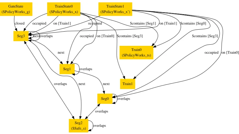
Figure1shows one such counterexample that the Analyzer produces, with the default theme.
Figure 3 shows the same counterexample with a theme produced by an expert, and Figure5
shows the counterexample with our inferred theme. The latter two figures are clearly more comprehensible than the default.
The uncustomized (default) diagram is dense and hard to comprehend. The ternary relations are particularly hard to follow. Furthermore, the nodes all look the same, and as such it is difficult to quickly differentiate trains from segments. It isn’t clear from the diagram why this scenario represents a counterexample to our claim or if the scenario is even well-formed.
Other default settings are possible, but produce results that are not noticeably better. For
example, in Figure2, relations are displayed, not as edges between nodes, but as labels on the
nodes themselves. While the diagram is less cluttered, the structure has been lost, and the user
might as well read a text dump of the solution. Neither the settings that produced Figure 1or
Figure3shows a custom visualization developed by an experienced Alloy user. This repre-sentation demonstrates several key decisions by the user:
• Sets are disambiguated by color and shape as well as by name – gates are green diamonds,
track segments are gray rectangles, and trains are blue trapezoids.
• The relation names have been dropped, and the relationships are distinguished instead by
color. Black arcs indicate segment connections, red arcs indicate that two segments over-lap, green arcs indicate the segments that are blocked by the gate, and blue arcs indicate train locations.
• The two states of the solution (the pre-state and the post-state) are represented as two
dia-grams. This is done by aprojectionoverTrainState– any relation with aTrainState
column has that column dropped. This means, for example, that theonrelation (shown as
a red arc) is no longer a ternary relation fromTrainStatetoTraintoSegbut instead
a binary relation fromTraintoSeg. As a binary relation,onis now easy to understand
when drawn as an arc. It is now apparent that the solution involvesTrain0moving from
one segment to an adjacent one. (Projection is described in greater detail in section3.1.)
• The node labels have been shortened. One segment has been labeledproblem, because it
is the segment that violates theSafepredicate; it overlaps with (connects via gray arrows
to) two other segments containing trains. We can now see why this is an example of an unsafe situation.
• A more subtle decision is to choose the track connections (black arcs) and overlaps (red
arrows) as thespineof the diagram. Selecting these spine relations tells the layout tool to
use those relations as the backbone of the diagram when planning the layout. Since the track connections are the same in both states, the structure of the track segments appears the same in both states. Without this, the diagram might be laid out differently after each train move, even if only one arc had changed. Choosing a good spine helps keep the structure intact throughout the solution trace.
3
Properties
As illustrated in the above example, solutions to Alloy models are rendered visually as a directed graph, where each node represents an element in a set, and edge is a tuple in a relation. When the solution contains many set elements or many tuples, the resulting graph can be difficult to comprehend.
To remedy this, Alloy allows the user to customize the graph by configuring properties of the sets and relations in the model. For example, if a particular set is not relevant to the current solution, the user can choose to make its nodes invisible. If there are many sets, the user can choose to make the nodes of each set take on a different color.
In addition, Alloy allows properties to be inherited based on the set hierarchy in the Alloy
model. For example, if CheckingAccount and SavingsAccount are both subsets of
SavingsAccount nodes will automatically be red unless the user explicitly overrides their color.
Once the user has customized the diagram, the user can save these customizations in aTheme
file for future reuse. In total, there are 8 properties that the user can adjust for each set, and
9 properties for each relation. These properties can be divided into two categories: structural
properties that affect the overall layout of the nodes and edges, andpresentationalproperties that
affect the appearance of each node and edge individually.
3.1 Structural Properties
Structural properties affect the layout of the graph, including which nodes and edges are visible, and the positioning of nodes and edges to one another. They do not affect the visual qualities of individual nodes and edges.
Projection. Since Alloy models do not have an intrinsic notion of time, models involving state changes are often represented using higher-order relations. For example, the balance of a bank
account over time might be modeled by creating a user-defined set calledTime and a ternary
relation that maps each element in the setAccounttoTimetoInteger, representing each
account’s balance at each point in time.
Visually, however, the resulting graph will simultaneously show the account balances at all points in time in the same diagram. With a large model, this can be very confusing. To remedy this, Alloy allows the user to project the graph over sets. For example, if the user chooses to
project the graph over theTimeset, Alloy will construct multiple graphs (one for each element
ofTime) and allow the user to scroll through each graph individually. Intuitively, the graph for
an elementTime0will just show the balances of each account atTime0.
When chosen properly, projection can make the result much easier to comprehend. However, if the wrong set is chosen for projection, the result is useless. For example, while it makes sense
to project overTimeto see how the account balance changes over time, and it may also makes
sense to project overAccountto view the changes to each account individually, it probably
doesn’t make sense to project overInteger.
Spine Relations. When determining the layout of nodes and edges, the visualization facility presumes the diagram to contain a dominant hierarchical structure. The default visualization setting treats all relations in the model as part of a single dominant hierarchy. However, in most models only a few relations are part of that hierarchy; the rest represent interactions across the hierarchy.
For example, in a model of a file system, the ideal visualization would probably treat the directory hierarchy as part the dominant structure, but not the linking relationships between objects in the file system.
The relations that participate in the dominant hierarchy are known as the ‘spines’ of the dia-gram.
nodes, the diagram can become cluttered and confusing. This clutter can be greatly reduced by
representing the relation as anattribute instead of an edge. That is, while the default layout
represents the tuple(a,b)in relationras an arc between nodesaandblabelled “r”, making
ran attribute causes(a,b)to be shown as an additional label in nodeathat reads “r: b”.
3.2 Presentational Properties
In addition to the structural properties detailed above, there are various visualization properties that affect the appearance of individual nodes and edges, but not the overall layout. When chosen properly, they can greatly enhance the clarity of the resulting graph.
Color and Shape. One way to clearly distinguish nodes visually is to assign different colors and shapes. In some domains, there may be existing conventions for what shapes to use for different type of objects in the model. Furthermore, sometimes it makes aesthetic sense to choose one shape over another. For example, if a node has multiple text labels on it, the node will occupy less space if drawn as a rectangle rather than a circle. On the other hand, if a node has many incoming or outgoing edges, the arrow heads will spread out more evenly if the node is drawn as a circle rather than a square or rectangle.
Label. By default, Alloy uses the set and relation names in the original model as the node and edge label. However, to ensure unique naming, the names in the model are often more verbose. For a given diagram, shortening a long name like “parentDirectory” to “parent” can make a big difference in reducing clutter. In the extreme case, if there is only one relation in the model, it makes sense to use the empty label, because the user only needs to know the topology of the nodes rather than the name of the edge.
Numbering Nodes. To distinguish multiple elements in a set from one another, the visualizer appends a number to each node. For example, in a file system model, the solution containing
three files will contain three nodes labeled File0, File1, and File2. This numbering is
unnecessary when the user cares only about the topology of the graph rather than the exact atom that each node points to. In such a situation, the user can turn off the automatic numbering for
theFileset to reduce clutter. Furthermore, by not including the number, eachFilenode will
have the same label and thus the same width, which usually permits a more regular arrangement of the nodes on screen.
4
Property Inference
There are two kinds of entities for which our technique infers properties: setsand relations.
There are also two kinds of properties to infer: structural andpresentational. Sometimes our
Projection. Perhaps the most important structural property isprojection. Our inference selects a set to project over in the following manner: assign a score to each set; if there is a set that scores at least 2, project over the set with highest score; otherwise, if no set scores at least 2, then do not project. A set earns a point for each of the following: it is totally ordered (an ordering constraint appears in the model); it participates in a ternary relation, its name begins or ends with
any of the following distinguished strings:State,Tick,Time,TimeStep.
Projection is usually necessary for dynamic models: that is, models that describe how the
system changes over time. Consequently, the name of the set to project over usually refers to
time or state in some way. Note that merely having a name that begins or ends withStateis
not sufficient: the set must score another point on one of the other criteria to be used as the basis of projection, as well as scoring more points than any other set.
Enumerations. Alloy models, like programs, often make use of the typesafe enumeration de-sign pattern for a predefined set of named constants. Here’s an example one using an enumeration to models colours in Alloy:
abstract sig Colour {}
one sig Red, Green, Blue extends Colour {}
We infer that a collection of sets constitutes an enumeration if those sets are mutually disjoint singletons that exhaustively partition a common superset. We use the knowledge of enumerations to infer other structural and presentational properties:
• Binary relations whose target is an enumeration (ie, where the second column is an
enu-meration) are shown as attributes rather than as edges.
• Enumerations are hidden unless they are the source (first column) of some relation.
• Relations involving enumerations are not considered as spine candidates.
Spine Relations. A ‘homogeneous’ relation is one whose source and target sets may overlap. If a relation is homogeneous, then it probably represents a recursive, graph-like data-structure, and should be considered a spine of the diagram. If the model contains a homogeneous binary relation whose target is not an enumeration, it is used as a spine; otherwise, all relations are considered spines.
Node shape and colour. Node shape and colour are used to represent set and subset mem-bership information. We here use the term ‘set family’ to refer to a top-level set and all of its subsets. Each set family is assigned a unique colour. Each set within a set family is assigned a similar shape: eg, one set family may have octagon and hexagon shapes, while another set family might have rectangle and trapezoid shapes. It would also be plausible to assign each set family a unique shape, and use different hues of the same colour to distinguish subsets. We have not presently implemented this alternative.
(Technical Alloy note: Where we say ‘set’ in the above paragraph we mean AlloyType
Node and edge labels and numbering. By default, nodes and edges are properly named with their fully qualified name: ie, their individual name is prepended with the name of their model. However, having two sets or relations with the same name in different models is rare, and so we trim off the model name.
If there is only one visible edge (after projection), then there is no need to label it. Similarly, if there is only one visible set (after projection), then its instances do not need to be labelled (numbering will be sufficient).
Nodes representing singletons do not need to be numbered.
5
Evaluation
To evaluate our property inference, we applied our techniques to a collection of Alloy models that come bundled in the Alloy distribution. The distribution also contains a theme file for each model, prepared by an expert user of the visualizer. We then measured the distance of our inferred theme to the expert theme and the distance from the standard default theme to the expert theme, according to a distance metric described below.
In this section, we discuss the distance metric that we developed and present comparisons between the default, expert, and inferred themes. On most models in the collection, our inferred theme measured visually closer to the expert theme than did the default theme. We also evaluated the inferred themes qualitatively, and discuss this further below.
5.1 Distance Metric
Our distance metric approximates the visual difference between two themes. To the first order, it simply counts the number of visualization properties that differ between two given themes and
reports the result. For example, if the nodes is a setNare numbered and labelled “N” in the first
theme, and un-numbered labelled “M” in the second, then our metric would count two setting changes (the numbering and label name settings) as the distance between the two.
However, there are a some properties, namely projection, color, and shape, where merely counting a change in their value does not accurately reflect the subsequent visualization differ-ences that change will effect. While projection over a set is controlled by a single setting that can be activated with a click of the mouse, it has extensive visual repercussions. As explained in
Section3.1, projection has the effect of turning one diagram into a sequence of of diagrams, and
in doing so, it can add sets and remove relations from the visual model.
To account for the extensive visual differences introduced by projection, the metric adds the sum of the number of sets and relations that are created and destroyed by the projection to the
overall distance between themes. Consider, for example, a model with setsAandBand a relation
rfromAtoB. Projection over the setAtransformsrfrom a relation to a set, so our metric adds
two additional units to the distance due to this projection, one for the removal of the relationr
and one for the addition of the setr.
A complication with measuring color and shape differences arises from color and shape
iso-morphisms. For example, if one theme colors elements in setAred and those is setBblue, and
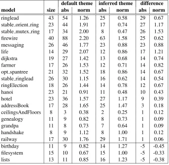
Table 1: Distances of the Default and Inferred Themes from the Ideal Theme
default theme inferred theme difference
model size abs norm abs norm abs norm
ringlead 43 54 1.26 25 0.58 29 0.67
stable orient ring 23 44 1.91 17 0.74 27 1.17
stable mutex ring 17 34 2.00 8 0.47 26 1.53
firewire 40 88 2.20 63 1.58 25 0.62
messaging 26 46 1.77 23 0.88 23 0.88
life 14 29 2.07 12 0.86 17 1.21
dijkstra 19 27 1.42 13 0.68 14 0.74
farmer 17 26 1.53 12 0.71 14 0.82
opt spantree 21 32 1.52 18 0.86 14 0.67
stable ringlead 26 30 1.15 16 0.62 14 0.54
ringElection 18 26 1.44 14 0.78 12 0.67
hanoi 23 21 0.91 11 0.48 10 0.43
hotel 23 36 1.57 27 1.17 9 0.39
addressBook 17 28 1.65 25 1.47 3 0.18
ceilingsAndFloors 8 3 0.38 2 0.25 1 0.12
genealogy 11 9 0.82 8 0.73 1 0.09
grandpa 11 8 0.73 7 0.64 1 0.09
handshake 8 9 1.12 8 1.00 1 0.12
railway 17 30 1.76 29 1.71 1 0.06
birthday 11 9 0.82 14 1.27 -5 -0.45
filesystem 15 10 0.67 15 1.00 -5 -0.33
lists 13 11 0.85 16 1.23 -5 -0.38
measure the distance between two colorings, the metric finds the color-to-color bijection that minimizes the number of miscolored nodes. Similarly, to find the distance between two shape configurations, the metric finds the shape-to-shape bijection that minimizes the number of mis-shaped nodes.
5.2 Quantitative Evaluation
The collection of models in the Alloy distribution come from a variety of domains and vary
greatly in size and complexity. Some, such asbirthday, are simple toy models typically
in-troduced in Alloy tutorials for novices, and some are models of famous puzzles, such ashanoi,
which formulates the Towers of Hanoi problem. Others are real-world systems, like the
rail-way gate policy described inrailway; textbook algorithms, such as the formulation Dijkstra’s
shortest path algorithm in dijkstra; and case studies of deployed protocols, including the
Firewire leader election protocol infirewire.
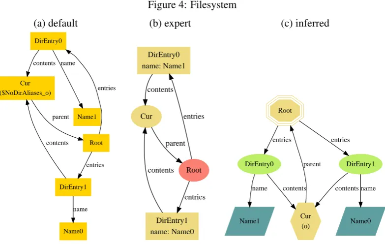
Figure 4: Filesystem
(a) default (b) expert (c) inferred
DirEntry0
Cur ($NoDirAliases_o)
contents
Name1 name
Root parent
DirEntry1 contents
Name0 name
entries
entries
DirEntry0 name: Name1
Cur contents
Root parent
DirEntry1 name: Name0 contents
entries
entries
DirEntry0
Cur (o) contents
Name1 name
DirEntry1
contents
Name0 name Root
entries
parent entries
The “size” column contains a measure of the size of the model, calculated as the number entities (sets and relations) it contains, and is suggestive of the model’s complexity. The third column shows the absolute distance from the default theme to the expert theme, as computed by our metric. The fourth column contains that absolute distance, normalized by the size of the model. The fifth and sixth columns show the distance from our inferred theme to the expert theme, both in absolute and normalized form. The last columns show the difference between the default-to-expert distance and the inferred-to-default-to-expert distance, both absolute and normalized.
As shown in Table1, for 19 of the 22 models, our inferred visualization theme came strictly
closer to the expert theme. For the remaining three, the inferred theme fell slightly behind the default theme, according to our metric.
5.3 Qualitative Evaluation
While the quantitative measurements estimate the proximity of one theme to another, ultimately what we care about is how the inferred themes looks to the human eye. In this section we visually
review three models that form a representative sample of how Alloy is commonly used: astatic
model (filesystem), adynamic transition model (railway), and a dynamic trace model
(ringlead). These are presented in order of increasing complexity, which also turns out to be the order of increasing success of our inference technique.
Filesystem Model. The filesystemmodel is one of the three models on which our infer-ence measured worse than the default settings. An instance rendered with the default, expert, and
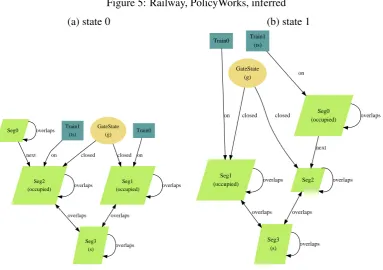
Figure 5: Railway, PolicyWorks, inferred
(a) state 0 (b) state 1
GateState (g)
Seg1 (occupied)
closed
Seg2 (occupied)
closed
overlaps
Seg3 (s)
overlaps overlaps
overlaps Seg0
next
overlaps Train0
on Train1
(ts)
on
overlaps
GateState (g)
Seg1 (occupied)
closed
Seg2 closed
overlaps
Seg3 (s) overlaps
overlaps
overlaps Seg0 (occupied)
next
overlaps Train0
on
Train1 (ts)
on
overlaps
a diagram that is already comprehensible, and the expert improves upon the default with some
color and shape changes and by showing thenamerelation as an attribute instead of an edge.
Despite the quantitative measurement, we feel that the inferred visualization is superior to the default because the visual hierarchy corresponds to the hierarchy of the modelled file system (due to the appropriate selection of spine relation). The “expert” visualization should have arguably made this choice as well, demonstrating that the automatic inference can out-perform experts in some respects.
Railway Model. We return to therailwaymodel presented in Section2. The default theme
and expert themes were given earlier in Figure1(a) and Figure3, respectively, and the inferred
theme is now shown in Figure5. Like the expert theme, our inferred theme includes a projection
over the setTrainState, but does not manage to infer the aesthetically-pleasing colors of the
expert.
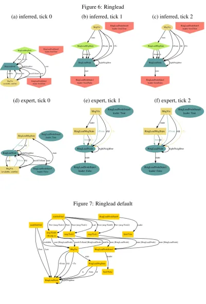
Ringlead Model. Lastly, we look atringlead, the model on which our inferred theme most out-performed the default theme. An example rendered with the default theme, shown in
Fig-ure7, is a tangled web of nodes and edges, and its meaning is hard to decipher. Both the inferred
and the expert themes (Figure6) project over the set of ticks, and they look fairly similar and far
Figure 6: Ringlead
(a) inferred, tick 0 (b) inferred, tick 1 (c) inferred, tick 2
RingLeadMsgState
RingLeadNode from id to
rightNeighbor MsgViz (available, sentOn) needsToSend sent RingLeadNodeState1 leader: bool/False state state
vTo vFrom vId
RingLeadNodeState0 leader: bool/True RingLeadMsgState RingLeadNode fromid to rightNeighbor RingLeadNodeState1 leader: bool/False state MsgViz state
vFrom vId vTo RingLeadNodeState0 leader: bool/True RingLeadMsgState RingLeadNode fromid to rightNeighbor RingLeadNodeState1 leader: bool/False state MsgViz state
vFrom vId vTo RingLeadNodeState0
leader: bool/True
(d) expert, tick 0 (e) expert, tick 1 (f) expert, tick 2
RingLeadMsgState
RingLeadNode
from idto
rightNeighbor MsgViz (available, sentOn) needsToSend sent RingLeadNodeState1 leader: False state state
vTo vFromvId
RingLeadNodeState0 leader: True
RingLeadMsgState
RingLeadNode
fromidto
rightNeighbor RingLeadNodeState1 leader: False state MsgViz state
vFromvIdvTo RingLeadNodeState0
leader: True
RingLeadMsgState
RingLeadNode
fromidto
rightNeighbor RingLeadNodeState1 leader: False state MsgViz state
vFromvIdvTo RingLeadNodeState0
leader: True
Figure 7: Ringlead default
msg/Tick0 ($Loop_t)
MsgViz
available sent [RingLeadNode]needsToSend [RingLeadNode]
RingLeadNodeState1 state [RingLeadNode] sentOn
RingLeadNode
vFrom vId vTo RingLeadMsgState state nodeOrd/Ord
First Last
rightNeighbor tickOrd/Ord
Prev [msg/Tick1] First
msg/Tick2
Next [msg/Tick1] Last
msg/Tick1
Next [msg/Tick0] Prev [msg/Tick2]
to from id
6
Discussion
A key observation from our evaluation is that the bigger and more complex the model, the greater the benefit of the automatic theme inference. In hindsight, this is not surprising. Instances of simples models are usually relatively easy to understand, so extensive customization beyond the default is usually not needed. As models become more complex, however, detailed customization becomes increasingly important in order to untangle and decipher the diagrammatic webs.
We also observed that the appropriate structural properties of a visualization are more easily and reliably inferred compared to the presentational ones. If, for example, the model exhibits
some of the tell-tale signs of being dynamic (discussed in Section4), then a projection should
almost certainly be applied. Compared to such structural properties, presentational characteris-tics are more likely to be arbitrary matters of taste. In a model of a file system, for instance, a user could choose to distinguish files from folders using different colors, shapes, labels, or some combination of all three.
The evaluation in this study focused on demonstrating the basic utility of our inference tech-nique. We have demonstrated that our inference technique produces better visualizations than the generic defaults in almost all cases. The ultimate objective of this project is to capture and mechanize the behaviour of expert users. Future work may include an objective qualitative study of how expert users customize visualization themes.
Acknowledgements:
This material is based upon work supported by the National Science Foundation under grants:
National Science Foundation,Deep and Scalable Analysis of Software, award number 0541183;
National Science Foundation ITR Programme,SoD Collaborative Research: Constraint-based
Architecture Evaluation, with Dewayne Perry, Sarfraz Khurshid and James Browne, award
num-ber 0438897: National Science Foundation ITR Programme, Safety Mechanisms for Medical
Software, with Michael Ernst and Martin Rinard, award number 0325283.
Bibliography
[GKN] E. Gansner, E. Koutsofios, S. North. Graphviz Website. http://graphviz.org
[Jac00] D. Jackson. Automating First-Order Relational Logic. InProceedings ACM SIGSOFT
Conference on Foundations of Software Engineering. San Diego, November 2000.
[Jac06] D. Jackson. Software Abstractions: Logic, Language, and Analysis. The MIT Press,
Cambridge, Mass., Apr. 2006.
[Lin02] L. Lin. Visualization Framework for Software Design Analysis. Master’s thesis, Mas-sachusetts Institute of Technology, 2002.
[Sof] Software Design Group. Alloy Website.