Volume 73 (2016)
Graph Computation Models
Selected Revised Papers from GCM 2015
Proving Correctness of Graph Programs
Relative to Recursively Nested Conditions
Nils Erik Flick
20 pages
Guest Editors: Detlef Plump
Managing Editors: Tiziana Margaria, Julia Padberg, Gabriele Taentzer
Proving Correctness of Graph Programs
Relative to Recursively Nested Conditions
Nils Erik Flick∗
Carl von Ossietzky Universität, 26111 Oldenburg, Germany,
Abstract: We propose a new specification language for the proof-based approach
to verification of graph programs by introducingµ-conditions as an alternative to
existing formalisms which can express many non-local properties of interest. The contributions of this paper are the lifting of constructions from nested conditions to the new, more expressive conditions and a proof calculus for partial correctness relative toµ-conditions. Most importantly, we prove the correctness of a new
con-struction to compute weakest preconditions with respect to finite graph programs.
Keywords: correctness, graph programs, non-local graph conditions, weakest
pre-condition calculus, proof calculus
1
Introduction
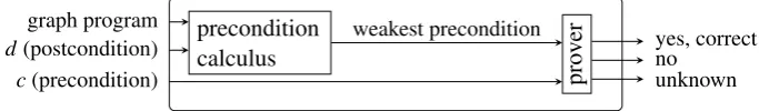
Graph transformations provide a formal way to model the graph-based behaviour of a wide range of systems by way of diagrams, amenable to formal verification. One approach to verification proceeds via model checking of abstractions, notably Gadducci et al., Baldan et al., König et al., Rensink et al. [GHK98,BKK03,KK06, RD06]. This can be contrasted with the proof-based approaches of Habel, Pennemann and Rensink [HPR06,HP09] and Poskitt and Plump [PP13]. Here, state properties are expressed by nested graph conditions, and a program can be proved correct with respect to a preconditioncand a postconditiond. The following figure presents a schematic overview of the approach, which is also our starting point:
precondition calculus
pro
v
er
graph program weakest precondition
d(postcondition)
c(precondition)
yes, correct no
unknown
Figure 1: Overview of the proof-based verification approach
Correctness proofs are done in the style of Dijkstra’s [Dij76] predicate transformer approach in Pennemann’s thesis [Pen09], while Poskitt’s thesis [Pos13] features a Hoare [Hoa83] logic for partial and total correctness. Both works are based on nested conditions, which cannot ex-press non-local properties of graphs, such as connectivity. In this paper, we consider non-local properties, and we present an extension to the proof calculus from [Pen09]. Our formalism is an extension of nested conditions by recursive definitions. Several extensions of nested graph
conditions to non-local conditions already exist (Radke [Rad13], Poskitt and Plump [PP14]). We argue that as opposed to the former, ours offers a weakest precondition calculus that can handle any condition expressible in it. As compared to the latter, which relies more heavily on expressing properties directly in (monadic second-order) logic, ours is more closely related to nested conditions and shares the same basic methodology. Thusµ-conditions offer a viewpoint
sufficiently different from existing ones to be worth investigating.
This paper is structured as follows:Section 2recalls graph programs and conditions.Section 3
introducesµ-conditions andSection 4defines correctness underµ-conditions and the proof
cal-culus, together with proofs of the results and a (small) exemplary application of the method.
Section 5provides context by listing related work.Section 6concludes with an outlook.
2
Graph Conditions and Programs
In this section, we introduce graph conditions and graph programs. We assume familiarity with graph transformation systems in the sense of Ehrig et al. [EEPT06], and the basic notions of category theory. For practical approaches to semi-automatic theorem proving in this context, we also refer the reader to Pennemann [Pen09]. In this paper, all graphs are assumed to be finite.
Notation The domain and codomain of a morphism f :G→H are denoted bydom(f) =G andcod(f) =H. Curly arrows f :G,→Hdenote injective morphisms (monomorphisms) while double-ended arrows f :GHdenote surjective ones (epimorphisms).Mdenotes the class of all graph monomorphisms. Anisomorphismof graphs is both a mono- and an epimorphism. A
partial morphismis a pair of monomorphisms with the same domain. /0denotes the empty graph.
Let us recall nested conditions, initially due to Habel and Pennemann. Finite nested conditions are known to be equally expressive as graph-interpreted first-order predicate logic.
Definition 1(Nested Graph Conditions) Let Cond be the class of nested conditions, defined
inductively as follows (whereP,C0,Care graphs):
• IfJis a countable set and for all j∈J,cjis a condition(overP), thenWj∈Jcjis a condition (overP). This includes the caseJ=/0(for anyP).
• Ifcis a condition(overP), then¬cis also a condition(overP).
• Ifa:P,→C0 is a monomorphism, ι :C,→C0 is a monomorphism andc0 is a condition
(overC), then∃(a,ι,c0)is a condition(overP).
Notation We callc0adirect subconditionof∃(α,ι,c0),¬c0andc0∨c00and usesubconditionfor the reflexive and transitive closure of this syntactically defined relation. Ifcis a condition over P, thenPis itstype1, denotedc:P, andCondP is the class of all conditions overP. The usual
abbreviations define the other standard operators: V is¬W
¬,∀is¬∃¬. No morphism satisfies the disjunction over the empty index set. To avoid special cases, we write it as⊥(false), and> (true) for¬⊥, though technically for each graphPthere is one⊥:Pand one >:P. We write ∃(a)for∃(a,ι,>),∃(a,c)for∃(a,idcod(a),c)and∃−1(ι,c)for∃(idcod(ι),ι,c).
With finite index sets, one obtains thefinitenested conditions. The morphismι serves to
unse-lect2a part ofC0. Our extension is similar to lax conditions [RAB+15], but slighter in scope.
Definition 2(Satisfaction) A monomorphism f :P,→G satisfies a conditionc:P, denoted
f |=c, iffc=>,c=¬c0 and f 6|=c0, orc=W
j∈Jcj and there is a j∈J such that f |=cj, or
c=∃(a,ι,c0)(wherea:P,→C0,ι:C,→C0,c0:C) and there exists a monomorphismq:C0,→G
such that f =q◦aandq◦ι|=c0.
∃(P C0 C, )
G
a ι
q
f q◦
ι
c0 |=
A graphGsatisfies a conditionc: /0 if and only if the unique morphism /0,→Gsatisfiesc.
Notation The symbol≡denotes logical equivalence, i.e. for conditionsc,c0:P, c≡c0 if and only if for all monomorphismsmwith domainP,⇒m|=c⇔m|=c0.
Remark1 (No Added Expressivity) Our conditions withι are equally expressive as the nested conditions defined in [Pen09]. The proof, omitted, relies on the transformationAfrom [Pen09].
Notation As one can see inFig. 2, the notation for graph conditions often only depicts source or target graphs of morphisms. The small blue numbers show the morphisms’ node mappings. We also adopt the convention of representing the morphismι in a situation∃(a,ι,xi)implicitly:
we prefer to annotate the variable’s type graph with the images of items underι in parentheses.
∃
/0,→ 1 2 ←- 2 ,¬∃
2
,→ 2 ←- 2 ,>
≡ ∃
1 2
,¬∃
2
Figure 2: A nested graph condition, in full and in abbreviated notation (stating the existence of two nodes linked by an edge, the second node not having a self-loop).
Next, we introduce graph transformations. We follow the double pushout approach with injec-tive rules and injecinjec-tive matches. For technical reasons, we define graph transformations in terms of four elementary steps, namely selection, deletion, addition and unselection. Deletion and addition always apply to a selected subgraph, and selection and unselection allow the selection to be changed. skip is a no-op used in the definition of sequential composition. The definition below allows for somewhat more general combinations of the basic steps, which cannot be ex-pressed as sets of graph transformation rules. Another reason for breaking up rules into more elementary steps is to make constructions and proofs easier to follow. Its only complication is that programs can only be composed if they agree on the currently selected subgraph, called the
interface. This ensures that an addition is performed in the same place as the deletion. A graph transformation rule is then nothing else than a selection; a deletion; an addition; an unselection.
The semantics of a graph program is a triple of two monomorphisms and one partial morphism. The two monomorphisms represent the selected subgraphs before and after the execution of the
2We will use the term “unselection” anytime a morphism is used in the inverse direction: inDef. 1, the morphism ι
program respectively, and the partial morphism records the changes effected by the program. Our programs are a proper subset of those in Pennemann [Pen09], and use the same semantics.
Definition 3(Graph Programs) In the following table,x,l,r,y,minandmout are
monomorph-isms, withx,l,randyarbitrarily chosen to define a program step, while theinterfaces min(input)
andmout (output) are universally quantified in the set comprehensions that appear in the
defini-tions below. Each triple(min,mout,(pl,pr))has cod(pl) =dom(min)and cod(pr) =dom(mout).
Name ProgramP SemanticsJPK
selection Sel(x) {(min,mout,x)|mout◦x=min}
deletion Del(l) {(min,mout,l−1)| ∃l0,(mout,l,min,l0)pushout}
addition Add(r) {(min,mout,r)| ∃r0,(min,r,mout,r0)pushout}
unselection U ns(y) {(min,mout,y−1)|mout=min◦y}
skip skip {(m,m,iddom(m))|m∈M}
IfPandQare graph programs, so are their disjunction{P,Q}and sequenceP;Q. The seman-tics of disjunction is a set unionJPK∪JQKand the semantics of sequence isJP;QK={(m,m
0,p)
| ∃(m,m00,p0)∈JPK,(m00,m0,p00)∈JQK,p=p0;p00}, where partial morphismsp0= (l1,r1),p00= (l2,r2)compose as p0;p00= (l1◦l20,r2◦r01)using the pullback(r01,l20) of(r1,l2). IfPis a graph program, so is itsiteration P∗:JP
∗
K=
S
j∈NJP
j
KwhereP
j=P;Pj−1for j≥1 andP0=skip.
Remark2 The definitions generalise the state transitions in plain graph transformation: a rule
ρ= (L←l-K,→r R)is exactly simulated by the programSel(/0,→L);Del(l);Add(r);U ns(/0,→R).
3
µ
-Conditions
In this section, we define µ-conditions on the basis of nested graph conditions. As opposed
to nested conditions, the ones defined here can express path and connectivity properties, which frequently arise in the study of the correctness of programs with recursive data structures, or in the modelling of networks. We then define and prove the correctness of some basic constructions. An example is provided at the end of this section to illustrate the constructions step by step.
3.1 Definingµ-Conditions
Nested conditions are a very successful approach to the specification of graph properties for verification. However, they cannot express non-local properties such as connectedness. Our idea is to generalise nested conditions to capture certain non-local properties by adding recursion. The resulting formalism is similar to first order fixed point logics, see e.g. Kreutzer [Kre02].
The reader might want to compare our µ-conditions to a distinct formalism for expressing
non-local properties, the very powerful grammar-based HR∗conditions of Radke [Rad13]. We argue thatµ-conditions are worth looking into despite the availability of strong contenders for an extension of nested conditions to non-local properties, such as MSO-conditions [PP14] because our approach provides a new and different generalisation of nested conditions, also is it not obvious how the respective expressivities compare.3 Specifically, we show in this section that
the weakest liberal precondition transformation, core of the Dijkstra-style approach, carries over.
Notation Sequences (of graphs, placeholders, morphisms) are written with a vector arrow~P,~x,
~f, and their components are numbered starting from 1. The length of a sequence~Pis denoted
byk~Pk. Indexed typewriter lettersx1 stand for placeholders, i.e. variables. The notationc:P
indicating thatchas typePis also extended to sequences:~c:~P(providedk~ck=k~Pk).
To define fixed point conditions, we need something to take fixed points of, and to enforce existence and uniqueness. Choosing a partial order on Cond~P, one can define monotonic
oper-ators on Cond~P. The semantics of satisfaction already defines a pre-order: c≤c
0 if and only if
every morphism that satisfiescalso satisfiesc0, which is obviously transitive and reflexive. As in every pre-order,≤ ∩ ≤−1 is an equivalence relation compatible with≤and comparing rep-resentants via≤partially orders its equivalence classes. We introduce variables as placeholders where further conditions can be substituted4. To represent systems of simultaneous equations, we work on tuples of conditions. If~P=P1, . . . ,Pk~Pk is a sequence of graphs, then Cond~P is the
set of allk~Pk-tuples~cof conditions, whosei-th element is a condition over thei-th graph of~P. Satisfaction is defined component-wise:~f|=~cif and only if∀k∈ {1, . . . ,k~Pk} fk|=ck.
DisjunctionsV
and conjunctionsW
of countable sets of CondPconditions, which by definition
exist for anyP, are easily seen to be least upper resp. greatest lower bounds of the sets. This makes Cond≡P a complete lattice. Let Cond~P be ordered with the product order by defining
~f |=~cto be true when the conjunction holds. This again induces a partial order on the set of
equivalence classes, Cond≡~P. Thus, Cond≡~Pis also a complete lattice, and a monotonic operator Fhas a least fixed point (lfp), given by the limit of~Fn(−→⊥)for alln∈N, by the Knaster-Tarski theorem [Tar55]. This is crucial in the definition of a µ-condition. We extend the inductive
definitionDef. 1by placeholders, and define substitutions of conditions for placeholders:
Definition 4(Graph Conditions with Placeholders) Given a graphPand a finite sequence~Pof graphs, acondition with placeholders from~PoverPis a (graph) condition with placeholders is either∃(a,ι,c), or¬c, orWj∈Jcj, orxi, 1≤i≤ kP~kwherexiis a variable of typePi.
Definition 5(Substitution) IfFis a condition with placeholders~xof typesP~ and~c∈Cond~P, thenF[~x/~c]is obtained by substitutingcifor each occurrence ofxifor alli∈ {1,...,k~Pk}.
Satisfaction of such a condition by a morphism fis defined relative to avaluationval, which is an assignment of>or⊥to each monomorphism of the type graph of the variable into cod(f), by
f |=xiiff val(xi) =>(where dom(f) =Piandxi:Pi). As discussed above, a lfp shall be defined
only up to logical equivalence. To guarantee its existence, the operator must be monotonic (~c≤~d⇒~F(~c)≤~F(d~)for any~c, ~d∈Cond~P). The following remark is very useful:
Remark3 The least fixed point of~Fis equivalent toW
n∈N~Fn(
− →
⊥).
Proof. This is a fixed point because~F(W
n∈N~Fn(
− →
⊥)) =W
n∈N−{0}~Fn(
− →
⊥) =⊥∨W
n∈N−{0}~Fn(
− →
⊥)
4Note that in our approach variables stand for subconditions, not for attributes or parts of graphs. Wherever confusion
=W
n∈N~Fn(
− →
⊥). It is the least fixed point because any other fixed point must also be a least upper bound of all~Fn(−→⊥)and therefore greater or equal to the one proposed.
Definition 6(µ-Condition) Given a finite list~Pand conditions{Fi}i∈{1,...,k~Pk}with
placehold-ers~x:~P(Fi having typePi and so on), thenµ[~x]~F(~x)denotes the least fixed point (lfp) of the operator that to any~cassigns~F[~x/~c]. Aµ-condition is a pair(b,l) consisting of a condition
with placeholdersb, and a finite list of pairs l= (xi,Fi(~x))of a variablexi:Piand a condition Fi(~x):Pi, with placeholders from~x, for some graphPi, such that~Fis monotonic.
We allowµ-conditions with open variables (i.e. not occurring as left-hand sides). For a least
fixed point of a subset of variables to exist, the system of equations must correspond to a mono-tonic operator underanyvaluation of the open variables. An operator is said to be monotonicin
a subset of variables when it is monotonic under any valuation of the remaining variables.
Notation We write the list of pairsl= (xi,Fi(~x))i∈{1,...,k~Pk}as a system of equations~x=~F(~x).
We callbthemain bodyandl therecursive specificationof(b,l) (andFi(~x) thebodyorright
hand sideof the variablexiinl, or thei-thcomponentof~F), and~F(~c)is understood as
substitu-tion of condisubstitu-tions~cfor the variables~x.~Fis said todefinethe variables~x.
Such systems of equations may be used in a broader sense, to define nested fixed points:
Definition 7(Transitive Variable Use) Let {Fi}i∈I} be a list of conditions as inDef. 6. The
userelation of F, ;F, is defined on literals{xi,¬xi}i∈I by xi;F xj (¬xj)iff xj occurs as a
subcondition under an even (odd) number of negations inFi. Thetransitive use pathsofFare
all sequences of literalsπp1...πpm such that∀1≤i<m.πpi ;Fπpi+1 and∀1<j<m.πpm 6=πpj.
Lemma 1(Nested Fixed Points) Given conditions with placeholders {Fi(~x)}i∈I, if there is a
partitioning I=I1]I2with~x1={~xi}i∈I1 and~x2={~xi}i∈I2 such that{Fi}i∈I1 does not use
vari-ables of~x2, then ifµ[~x]~F(~x)exists it is equivalent toµ[~x1]~FI1(~x1)with~FI1(x~1) =µ[~x2]~FI2(~x2,~x1).
Proof. Immediate from the definition of least fixed point.
Definition 8(Stratification) Fis said to bestratifiedif there is a decomposition into~FI1, ...,~FIn
such that each~FIm is monotonic in~xIm and there are no variablesxi; +
F xj, j∈Ij,i∈Ii, j<i.
Such a decomposition is termed astratificationof~Fand the~FIm arestrataof~F.
Note that the possible decompositions only depend on the strict partial order of transitive variable use;+F. The order and decomposition of fixed points on;+F-incomparable subsets of variables does not matter byLemma 1. Therefore there is no ambiguity in presenting a nested fixed point as a system of equations without explicit stratification. Monotonicity and stratification can be enforced syntactically and we only consider suchµ-conditions to be well-formed:
Proof. We prove by structural induction thatFi(~x) is monotonic in xj under even numbers of
negations and antitonic under odd numbers, i.e. c≤d⇒Fi[xj/c]≤Fi[xj/d]resp. c≤d⇒ Fi[xj/c]≥Fi[xj/d]. The base case is either>orxj0, j6= j0 (trivial), or xj (monotonic). The
other cases are negation, disjunction and existential quantifiers. Examining Def. 2, negation interchanges both even/odd and monotonicity/antitonicity. Disjunction, defined via propositional logic too, is monotonic, quantifiers∃(a,ι,c0)are monotonic inc0. Hence the latter two cases do not affect either property. If all components of~Fare monotonic inxj, then so is~F. Porting the
argument to stratified systems merely requires checking the monotonicity of each stratum.
Remark5 (First Example:µ-Conditions are More General than Nested)
1. µ-conditions generalise nested conditions, consequently all examples for nested condi-tions are examples forµ-conditions (with no variables or equations).
2. µ-conditions are strictly more general than nested conditions: the following expresses the existence of a path of unknown length between two given nodes.
x1
1 2
where x1
1 2
= ∃
1 2
∨ ∃
1 2
3
,x1
1(3) 2(2)
It reads as follows: the word “where” stands between main body and equations. The only variable is x1. Its type graph is indicated in square brackets. The second existential quantifier uses a morphism to unselect node 1 and the sole edge: its source is the type graph of x1, which is syntactically required for using the variable in that place. The unselection morphism ι is not
written as an arrow, instead it is expressed in compact notation by appending small blue numbers in parentheses to the node numbers in its source graph to specify the mapping. To ease reading, we adopt the convention to always use the same layout for the type graph of a given variable.
Let us motivate the necessity of “unselection”. Thenesting depth n: Cond→Nis defined as
n(W
j∈Jcj) =max({0} ∪ {n(cj)| j∈J}),n(¬c) =n(c),n(∃(a,ι,c)) =n(c) +1, (n(xi) =0).
Lemma 2(Absorption) Any condition with placeholders c=∃(a,ι,c0)where a andι are iso-morphisms is equivalent to a condition of smaller nesting depth (or equal if n(c) =1).
Proof. Define the reduced conditionra,ι(c0)thus: ifc0= W
j∈Jcj, thenra,ι(c0) = W
j∈Jra,ι(cj). If
c0=¬c00, thenra,ι(c0) =¬ra,ι(c00). Ifc0=∃(a0,ι0,c00), thenra,ι(c0) =∃(a0◦ι−1◦a,c0). Directly
fromDef. 2,ra,ι(c
0)≡cand at the same time,n(r a,ι(c
0)) =n(c0) =n(c)−1. The only case where
nesting depth does not decrease is whenc0is a variable, resulting in nesting depth 1.
Remark6 (Whyι) Anyµ-conditionb|~x=~F(~x)whereι is the identity in all subconditions of band of the componentsFi(~x)is equivalent to a nested condition.
Proof. Decompose~FbyLemma 1such that each stratum~FIm only defines variables of the same
type. This is indeed possible since with no non-trivial unselection, a variable may transitively depend on itself only via a morphism that is both injective and surjective. Induction over the number of strata: for each~FIm, after each step of the lfp iteration, the nesting level can be reduced
byLemma 2whenever∃(a,ι,c)withaisomorphism occurs. Hence an equivalent condition of
form∃(a,ι,xi)with isomorphismsaandι. Finitely many distinct conditions of this form, hence
finitely many distinct Boolean combinations, exist. The monotonic operator~FIm thus converges
after finitely many steps to a finitely deeply nested condition with placeholders, for which the next stratum’s lfp, by induction hypothesis possessing the desired property, is substituted.
Definition 9(Satisfaction) b|~x=~F(~x)with~x:P~ is satisfied by f iff f |=b[~x/µ[P]F].
This means that theµ-conditionb|~x=~F(~x)can be understood by substituting the lfp solution of the system of equations~x=~F(~x)in the main bodyb(for stratified systems, use appropriate nested fixed points). Satisfaction ofµ-conditions with open variables is analogous to satisfaction
of conditions with placeholders, i.e. requires a valuation to be given.
Remark7 (Finite Nesting) By the “infinite disjunction” characterisation of the lfp, anyµ -con-dition is equivalent to an infinite nested con-con-dition. Infinitely deep nesting is not needed because the characterisation inRem. 3yields a countable disjunction offinitely deeplynested conditions.
A morphism satisfies a given µ-condition if and only if it satisfies the finite nested condition obtained by unrolling the recursive specification up to some finite depth:
Proposition 1(Satisfaction at Finite Depth) f |=b|~x=~F(~x)iff∃n∈N, f |=b[~x/~Fn( − →
⊥)].
Proof. The lfp is equivalent toW
i∈N~Fi(
− →
⊥), which is satisfied by f iff at least one~Fn(−→⊥)is.
Theorem 1(Deciding Satisfaction of µ-Conditions) Given a morphism f :P,→G and aµ
-condition c, it is decidable whether f satisfies c.
Proof. The following algorithmCheckMudecides f|=c. For the type graphPi of each variable
xi, list all monomorphismsmik:Pi,→G. Build a table which records in each column a Boolean
value for each pair(xi,mik). The entries in column j+1 are computed by evaluating satisfaction
of the right hand side corresponding to the row’s variable by the morphismmik associated with
the row, under the valuation given by column j. Stop after producing two adjacent columns with the same entries. Output the value of the main body under that valuation. The algorithm is cor-rect because the j-th column corresponds to satisfaction by~Fj(−→⊥), by definition. It terminates because of monotonicity: as values never change back to⊥from>while progressing through the columns, there is a finite number j∗∈Nsuch that~Fj
∗
is satisfied by f iff~Fj∗+1is.
3.2 Weakest Liberal Preconditions ofµ-conditions
In this subsection, we present a construction to compute the weakest liberal precondition of aµ
-condition with respect to any iteration-free graph programP(“liberal” means termination ofPis not implied. It is redundant in the absence of iteration, as only iteration causes non-termination).
Definition 10(Weakest Liberal Precondition) The weakest liberal precondition (wlp) ofcwith respect to the programP, Wlp(P,c), is the least condition with respect to implication such that
We show that under this assumption there is aµ-condition that expresses precisely the weakest
liberal precondition of a givenµ-condition with respect to a rule, and it can be computed. The
result is similar to the situation for nested conditions. To derive it, we use theshifttransformation
Am(c) from [Pen09] whose fundamental property is to transform any nested condition c into
another nested condition such thatm00|=Am(c)if and only ifm00◦m|=cfor all composable pairs
m00,mof monomorphisms (Lemma 5.4 from [Pen09]). Since this and similar constructions play an important role in this section, we recall the casec=∃(a,c0): if(m0,a0)is the pushout of(m,a), let Epi be the set of all epimorphismsewith domain cod(m0)that compose to monomorphisms
b:=e◦a0andr:=e◦m0. ThenAm(∃(a,c0)) =We∈Epi∃(b,Ar(c0)).
With help of the unselectionι in∃(a,ι,c), it is at first glance trivial to exhibit a weakest
lib-eral precondition with respect toU ns(y). However, to handle the addition and deletion steps, a construction becomes necessary that makes the affected subgraph explicit again. This informa-tion is crucial to obtain the weakest liberal precondiinforma-tion with respect toAdd(r)andDel(l)and must not be forgotten at any nesting level in order to obtain the correct result. To that aim, we define apartial shiftconstruction which makes sure that the type graph of the main body is never unselected in theµ-condition but is instead mapped in a consistent way as a subgraph of the type
graph of each variable. The following serves to obtain the new type graphs:
Construction1 (New type graphs for partial shift) We assume that an arbitrary total order on all graph morphisms is fixed. Ifc=b|~x=µ[~K]~F(~x)is a µ-condition, then for a variablexiof
~
K,XR,c(xi)is defined as the sequence of morphisms~f obtained as below, in ascending order.
The new list of variables ~K0 and their respective types ~P0 are obtained by concatenating all
XR,c(xi)of the variables ofK~ in order. The morphisms f are obtained from~P0 by collecting all epimorphisms that compose to monomorphisms with the pushout morphisms in the diagram:
/0 R
Pi X P0j
f
Lemma 3(Decomposing “exists”) ∃(a,ι,c)≡ ∃(a,∃−1(ι,c))
Proof. f |=∃(a,∃−1(
ι,c))⇔ ∃q∈M,f=q◦a∧q◦idcod(a)|=∃−1(ι,c) ⇔ ∃q∈M,f=q◦a∧ ∃q0∈M,q◦idcod(a)=q0◦idcod(ι)∧q0◦ι |=c0 ⇔ ∃q∈M,f=q◦a∧ ∃q0∈M,q=q0∧q0◦ι|=c0
⇔ ∃q∈M,f=q◦a∧q◦ι|=c0⇔ f |=∃(a,ι,c)
Construction2 (Partial shiftPx,y) Given monomorphismsx:P,→Handy:R,→H, we define
thepartial shiftofb|µ[~K]Fwith respect to(x,y)asPx,y(b|µ[~K]F):=Px,y(b)|µ[K~0]F0, where the new equations are obtained by applyingPf,y to the variables of the left hand sides with all
possible morphisms f fromR, as below, and accordingly to the right hand sides. On condition bodies,Px,yis defined as follows: Boolean combinations of conditions are transformed to the
cor-responding combinations of the transformed members.Px,y(xi):=x x,y
i ifxi:P, wherex x,y i :His
a new variable,H=cod(y). Quantification is processed separately from unselection (Lemma 3):
Px,y(∃(P a
,→C0,c0)) =W
domainH0that compose to monomorphismsr=e◦x0andb=e◦hwith the pushout morphisms (diagram below left). Px,y(∃−1(C0
ι
←-C,c0)) =∃−1(ι0,P
i,y0(c0)): form the pullback ofr◦ι and
b◦y, then pushout the obtained morphisms to(y0,i)(diagram below right):
P C0
H H0 E
R a
y h x x0
e b
r r◦y
C0 C
E J
R B
x ι
y
i ι0
y0
Remark8 ((Un)ambiguous Variable Contexts) Note that in aµ-condition it is not necessarily true that in all contexts wherexiis used, it appears with the same morphismR,→Pi(whereRis
the type ofb). It is however possible to equivalently transform everyµ-condition into a “normal form” that has that property. ApplyingPidR,idR will by construction result in aµ-condition with unambiguous inclusions R,→Pi for all variables (namely the morphisms from the sequences XR,c), and this property is also preserved by the constructions introduced later in this section.
Unreachable variables created byXandPcan be pruned to obtain an equivalentµ-condition.
Equivalence of conditions with placeholders (unlike µ-conditions) is defined for conditions
using the same sets of variables, as equivalence in the sense of nested conditions under any valuation. We extendAto conditions with placeholders by definingAm(x)to be∃(idcod(m),m,x)
ifx:P. We show below thatPx,y is equivalent toAx. The reason for introducingPx,y is to gain
precise control over the types of the variables in the transformed condition, which should all include the type graph of the main body. Intuitively, as this corresponds to the currently selected subgraph of a graph program, additions and deletions are applied to that subgraph and one must ensure that the changes apply to the wholeµ-condition. Three minor lemmata are required:
Lemma 4(Removal of Unselection) If c0 is a condition with placeholders, then ∃(a,ι,c0)≡ ∃(a,A(ι,c0))(A being Pennemann’s shift as described earlier in this subsection).
Proof. Using the fundamental property ofA, the nontrivial case being m|=∃(a,ι,c0)⇔ ∃q∈
M,q◦a=m∧q◦ι|=c0 ⇔ ∃q∈M,q◦a=m∧q|=A(ι,c0)⇔m|=∃(a,A(ι,c0)).
Lemma 5 (Shift composition and decomposition) Given two morphisms m00, m0, if m00◦m0 exists, then Am00◦m0(c)≡Am00(Am0(c))for all conditions (with placeholders) c.
Proof. f |=Am00◦m0(c)⇔ f◦m00◦m0|=c⇔ f◦m00|=Am0(c)⇔ f |=Am00(Am0(c))(Lemma 5.4 in
[Pen09])
Lemma 6 The conditionsPx,y(c)and Ax(c)are equivalent.
Proof. By induction over the recursion depth, and structural induction overc: Ifcis a variable symbolxi, then either recursion depth is 0 and the assertion is proved, since it is⊥, or it is true
because the right hand side of the equation forxi has the property. The case∃(a,ι,c0)of the
eand compositionsb,r): m|=Ax(∃(a,ι,c0))⇔m|=Ax(∃(a,A(ι,c0)))according toLemma 4 ⇔m|=W
∃(b,Ae◦x0(Aι(c0)))by Lemma 5.4 from [Pen09]
⇔m|=W∃(
b,Ae◦ι0(Ai(c0))byLemma 5(twice)⇔m|=W∃(b,e◦ι0,Ai(c0))byLemma 4
⇔m|=W
∃(b,e◦ι0,Pi,r0(c0))by induction hypothesis⇔m|=Px,r0(∃(a,ι,c0))byConstr. 2
We introduce two transformations δ0l(c), α0r(c) (based on auxiliary transformations δl,y(c)
andαr,y(c)). These are applied to main body and right hand sides and serve to compute the wlp
with respect to addition and deletion, respectively5, of aµ-condition that has already undergone
partial shift. Recall the statement ofRem. 8 that partial shift fixes inclusions from the current interface to each graph occurring in the condition (as domain or codomain of a morphismaorι).
When the conditioncobtained after partial shift is evaluated on a morphism to check satisfaction, the current interface is never unselected in the recursion but appears included in each variable type. The conditionα0r(c)stipulates the existence of cod(r)(theAdd(r)step’s input interface)
instead of dom(r)(the output interface), which is intuitively why it yields the correct expression of the wlp ofcwith respect toAdd(r). It might well be that an occurrence of cod(r)cannot have been obtained by a rule application because the pushout demanded by the semantics ofAdd(r) fails to exist, in which caseα0 eliminates a branch of the condition. Likewise, inδ0l(c), cod(l)
takes the place of dom(l)since this corresponds exactly to the effect of the stepDel(l).6
Definition 11(Transformations δ0 andα0) Letc:P be a condition with placeholders. If r: K,→Randy:R,→P(resp.l:K,→Landy:K,→P) are monomorphisms, thenδr,y(c)(αl,y(c)) is
defined as follows:δr,y(¬c) =¬δr,y(c)andδr,y(
W
j∈Jcj) =
W
j∈Jδr,y(cj)(respectively:αl,y(¬c) =
¬αl,y(c)andαl,y(Wj∈Jcj) =Wj∈Jαl.y(cj)). Forc=∃(a,ι,c0), decompose usingLemma 3:7
P C0
R
W X
K a
y
y0 h0 r h
a0 r0 r00
C0 C
R
X V
K ι
y y0 h0 r h
ι0
r0 r000
| {z }
δr,y(∃(a,c))andδr,y(∃−1(ι,c))
P C0
K
W X
L a
y
y0 h0 l h
a0 l0 l00
C0 C
K
X V
L ι
y y0 h0 l h
ι0
l00 l000
| {z }
αl,y(∃(a,c))andαl,y(∃−1(ι,c))
Case ofδr,y(∃(a,c)): if no pushout complement ofr andy0=a◦yexists, thenδr,y(c) =⊥.
Otherwise, obtain it as(x0,h0)and pullback(a,r0)to(a0,r00)with sourceW; this yields a unique morphismh fromK toW to make the diagram commute. Apply the special pushout-pullback lemma [EEPT06] to the compositionsh0=a0◦handy0=a◦yto see that the left and top squares in the diagram are pushouts. δr,y(∃(a,c)) =∃(a0,δr,y0(c0)). Case of δr,y(∃−1(ι,c)): Pullback (ι,r0)to(ι0,r000). The pullback property yields existence and uniqueness ofh0:K→V to make
the diagram commute.δr,y(∃−1(a,c)) =∃−1(ι0,δr,y0(c)).
Case ofαl,y(∃(a,c)): pushout(y,l)to(l0,h); pushout(l0,a)to(l00,a0). h0is obtained asa0◦h
5 The letters were chosen so as to indicate the effect of the transformation: to compute the wlp with respect to addition,δ0needs todeleteportions of the morphisms in the condition, and vice versa.
6In the case ofDel(l), it is possible that
δ0l(c)specifies an occurrence oflwhich cannot be the input of aDel(l)step,
hence to obtain the actual wlp, a nested condition expressing the applicability ofDel(l)must be adjoined toδ0l(c).
and the composed square is a pushout. αl,y(∃(a,c)) =∃(a0,αl,y0(c0)). Case ofαl,y(∃−1(ι,c)):
let(h,l00)be the pushout over(y,l)and(h0,l000)over(y0,l). The commuting morphism from the latter pushout object toX isι0.αl,y(∃−1(ι,c)) =∃−1(ι0,αl,y0(c0)).
For variables, δr,y(xi) = x0i is a new variable of type K, likewise αl(xi) has type L (see
Rem. 8). Finally,δ0r(c) =δr,id(Pid,id(c))andα0l(c) =αl,id(Pid,id(c)).
In contrast toP, the transformationsα0 andδ0 leave the number of variables unchanged. Only
the types of the variables are modified. We recall that for anyl:K,→L, there is a condition
∆(l) that expresses the possibility of effectingDel(l), i.e.∆(l) is satisfied exactly by the first components of tuples inJDel(l)K. We describe∆(l)only informally: f |=∆(l)states the
non-existence of edges that are inim(f)but incident to a node inim(f)−im(f◦l).
Now we have all ingredients for a weakest liberal precondition theorem forµ-conditions. The proofs again rely on the general theoretical framework of double-pushout rewriting [EEPT06].
Theorem 2(Weakest Liberal Precondition forµ-conditions) For each ruleρ, there is a trans-formationWlpρ that transforms µ-conditions toµ-conditions and assigns to each condition c such that m0|=c another conditionWlpρ(c)such that m|=Wlpρ(c)whenever(m,m0,p)∈JρK andWlpρ(c)is the least condition with respect to implication having this property.
Proof. We exhibit and prove the transformation in four steps, which compose to the full rule.
1. Wlp(U ns(y),c) =∃−1(y,c)
2. Wlp(Add(r),c) =δ0r(b)|µ~x0=~F0(~x0)wherec=b|µ~x=~F(~x), and~x0,~F0are obtained
by applyingδ0rto the main body and the equations (adapting the variable types).
3. Wlp(Del(l),c) =∆(l)⇒α0l(c)|µ~x0=~F0(~x0), new equations analogous toAdd(r)
4. Wlp(Sel(x,c0),c) =¬∃(x,(c0∧ ¬c))
The proof forSel(x,c0) is exactly as in [Pen09], while correctness of the first step,U ns(y), is immediate from the semantics. For steps 2 and 3, we proceed by inductively comparingcto Wlp(Del(l),c)resp. Wlp(Add(r),c), which in turn requires inductively comparing conditions with placeholders that appear in the main body and right hand sides. The outer induction over
N(see Rem. 3) compares the least fixed points. This takes care of the case of variables. The
induction hypothesis here states that the valuation at the current iteration satisfies the hypothesis. As the variables satisfy the system of equations, we show by induction over the nesting that the construction is correct for the right hand sides under any valuation satisfying the hypothesis.
The interesting case of the induction over the nesting lies in comparing satisfaction of∃(a,ι,c) toαl,y(∃(a,ι,c)), resp. δr,y(∃(a,ι,c)). The goal is to obtain bi-implications in both cases. The
G D
P C0
W X
L K l0 h
y a d
G D
P C0
W X
L K l∗ g
D G0
P C0
W X
K R
D G0
P C0
W X
K R
CaseJDel(l)K/α
0 Case
JAdd(r)K/δ
0
(min,mout,l−1)∈JDel(l)K,mout:K,→D,min:L,→G(as depicted in the diagram) andmout|=
∃(a,ι,c)viad: considerαl,y(c), whereyis the morphismK,→Pobtained from the partial shift
construction. Build the pushout over(l0,d)and compose it with the lower pushout square, which yields the outer pushout by uniqueness. The morphismg:W ,→Gobtained in the pushout and the unique commuting morphismq:X,→Gyield satisfaction.
(min,mout,l−1)∈JDel(l)K,mout:K,→D,min:L,→Gandmin|=αl,y(∃(a,ι,c))viag: pullback
l∗andgwith objectP0, consider the universal morphism fromKtoP0and conclude that since a canonical isomorphismP0∼=Pexists by uniqueness of the pushout complement (sinceh:L,→W
is a monomorphism [EEPT06]) yielding a morphismd:P,→Dto complete the pushout square by the special PO-PB lemma.
(min,mout,r)∈JAdd(r)K,mout:R,→G
0,m
in:K,→Dandmout |=∃(a,ι,c)viag0: pullback D,→G0andP,→G0with objectW0, then use the unique commuting morphismK,→W0 which yields a decomposition of the pushout square from the semantics, which by the special PO-PB lemma consists of pushouts and by uniqueness ofM-pushout complements impliesW ∼=W0.
(min,mout,r)∈JAdd(r)K, mout :R,→G
0,m
in:K,→Dandmin|=δr,y(∃(a,ι,c))viag, in the
same way as the opposite direction of theDel(l)case.
In the case ofDel(l), the condition for the pushout complement required by the semantics to exist is precisely∆(l). In the case of Add(r), the construction ofδ0 asserts the existence of
the pushout. From the induction hypothesis and universality of the morphisms constructed to complete the diagrams, the diagrams must commute and we conclude thatmout |=c⇔min|=
Wlp(Del(l),c), resp.mout |=c⇔min|=Wlp(Add(r),c)under the given circumstances.
3.3 A Weakest Liberal Precondition Example
In this subsection, we construct a weakest liberal precondition of a µ-condition step by step.
Fig. 3shows a single-rule graph program which matches a node with exactly one incoming and
one outgoing edge and replaces this by a single edge. The effect of the rule is to contract paths, and it can be applied as long as no other edges are attached to the middle node. Fig. 4shows a µ-condition whose weakest liberal precondition we wish to compute. It is a typical example
of aµ-condition, which evaluates to>on those graphs that are fully (directed-) connected, i.e.
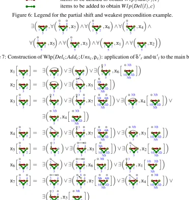
where any pair of nodes is linked by a directed path. InFig. 7andFig. 8, a partial shift has been applied to the condition (Wlp(U nsc,c4)) ofFig. 5, and the modifications the condition undergoes in the computation of the weakest precondition with respect toAddcandDelcare highlighted in various colours (seeFig. 6for a legend).Constr. 1has yielded a new list of variables8,x1, ...,x7,
8Although the original
Sel
/0,→ ;Del
1 3
2 ←
-1 2
;Add
,→ ;U ns
←-/0
Figure 3: A path-contracting ruleρcontract=Selc;Delc;Addc;U nsc.
∀
1 2 ,x1
where x1
1 2
=∃ 1 2
∨ ∃
1 2 3
,x1
1(3) 2(2)
Figure 4: Aµ-conditionc4= (b,l)expressing connectedness.
∃ 3 4
←-/0,∀
1 2 ,x1
where x1
1 2
=∃ 1 2
∨ ∃
1 2 3
,x1
1(3) 2(2)
Figure 5: Wlp(U nsc,c4). The nodes under the universal quantifier are not the same as those of the existential one, as these have been unselected: the type of the subcondition∀(...)is /0.
the corresponding equations are shown in Fig. 8, in abbreviated notation: variable types are suppressed in subconditions∃(a,ι,xi)if the mappingι from the type graph to the target ofais
the identity. No other simplifications were applied. We have highlighted the type of the main body of Wlp(U nsc,c4)throughoutFig. 7: edges drawn in red are deleted to compute Wlp(Addc
,Wlp(U nsc,c4))as per Def. 11; the green edges and nodes, not present initially, are added to compute Wlp(Delc,Wlp(Addc,Wlp(U nsc,c4)))as perDef. 11, which is obtained by adjoining
∆(l)⇒to the main body (∆(l)omitted inFig. 7as it is straightforward to compute); the yellow
nodes belong to both the red and green sets. A universal quantifier with /0,→Lcompletes the weakest precondition with respect to the rule, as for nested conditions [Pen09].
When following the construction through the nesting levels, please keep in mind that one may sometimes choose among isomorphic pushout objects and that the numbers of new nodes are arbitrary, but the nodes1,2and (as created by the transformationα0) 5are never “unselected”
and therefore present in every type graph occurring in the weakest preconditions, similarly for the edges (not numbered because their mapping is unambiguous in the example).
4
Correctness Relative to
µ
-conditions
In the previous section, we have shown how the weakest liberal precondition construction for nested conditions carries over toµ-conditions. The next task, for which we offer a partial solution
in this section, is to develop methods for the deduction of correctness relative toµ-conditions by
extending Pennemann’s proof calculusK. We recall thatKworks on nested conditions which are in conjunctive normal form at each nesting level; it features rules called (supporting)liftand (partial)resolve: the former serve to lift a member of a conjunction to a deeper nesting level, conjoining itsshiftto the subcondition of an existential quantifier, while the latter seek to derive contradictions. The ruledescendallows a member∃(a,⊥ ∧c)of a clause to be replaced by⊥.
4.1 A Proof Calculus forµ-conditions
node/edge decoration meaning
items (nodes and edges) selected forW l p(U ns(y),c) items to be deleted to obtainW l p(Add(r),c)
items to be added to obtainW l p(Del(l),c)
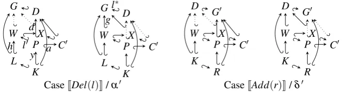
Figure 6: Legend for the partial shift and weakest precondition example.
∃ 1 2 5 ,∀ 1 2 3 4 5
,x7 ∧ ∀ 1 2 3 5 ,x6 ∧ ∀ 1 2 3 5 ,x4 ∧ ∀ 1 2 3 5
,x5 ∧ ∀ 1 2 5 3 ,x3 ∧ ∀ 1 2 5 ,x1 ∧ ∀ 1 2 5 ,x2
Figure 7: Construction of Wlp(Delc;Addc;U nsc,ρc): application ofδ0randα0lto the main body.
x1 h 1 2 5 i = ∃ 1 2 5 ∨ ∃ 1 2 5 ∨ ∃ 1 2 5 3 ,x6 h 1(1) 2(2) 3(3) 5(5) i x2 h 1 2 5 i = ∃ 1 2 5 ∨ ∃ 1 2 5 3 ,x5 h 1(1) 2(2) 5(5) 3(3) i x3 h 1 2 3 5 i = ∃ 1 2 3 5 ∨ ∃ 1 2 3 4 5 ,x7 h 1(1) 2(2) 5(5) 3(3) 4(4)i
∨ ∃ 1 2 5 3(3) ,x4 h 1(1) 2(2) 5(5) 3(3) i ∨ ∃ 1 2 5 3(3) ,x4 h 1(1) 2(2) 5(5) 3(3) i x4 h 1 2 5 3 i = ∃ 1 2 5 3 ∨ ∃ 1 2 3 4 5 ,x7 h 1(1) 2(2) 5(5) 3(3) 4(4) i
∨ ∃ 1 2 5 3(3) ,x3 h 1(1) 2(2) 5(5) 3(3) i x5 h 1 2 3 5 i = ∃ 1 2 3 5 ∨ ∃ 1 2 5 3 4 ,x5 h 1(1) 2(2) 5(5) 3(4) i ∨ ∃ 1 2 5 3
,x2 h 1(1) 2(2) 5(5) i x6 h 1 2 5 3 i = ∃ 1 2 5 3 ∨ ∃ 1 2 5 3 4 ,x6 h 1 2 5 3(4) i ∨ ∃ 1 2 5 3
,x1 h1(1) 2(2)
5(5) i x7 h 1 2 5 3 4i
= ∃ 1 2 5 3 4 ∨ ∃ 1 2 5 6 3 4 ,x7 h 1(1) 2(2) 5(5) 3(6) 4(4)i
∨ ∃ 1 2 5 3 4 ,x4 h 1(1) 2(2) 5(5) 3(4) i ∨ ∃ 1 2 5 3 4 ,x3 h 1(1) 2(2) 5(5) 3(4) i
Figure 8: Construction of Wlp(Delc;Addc;U nsc,ρc): equations for the variables.
Kµwe adopt all rules ofK. However dealing with recursive definitions requires an extension.
The strategy used in Pennemann’s PROCONtheorem prover [Pen09] (converting the condition to be refuted to a conjunctive normal form at each nesting level and deducing contradictions at the innermost nesting levels) is not applicable in the presence of recursion. Instead, we add all Boolean manipulations as rules, and propose an induction rule to deal with situations involving fixed points. This proved to be sufficient to handle all situations encountered in the examples.
We employ a sequent notation: the inference rules manipulatesequentsF,Γ`∆, whereFis a
system of equations,Γand∆are sets ofµ-condition bodies, with the intended meaning that the disjunction of∆can be deduced from the conjunction ofΓwhere the least fixed point solution of
expres-sion over natural numbers and identifiersn1, ..., which serve the important purpose of ensuring well-foundedness in the recursive refutation rule. Note that it is always sound to increment an annotation in an inference because by monotonicity, Fin(~⊥)⇒F
n+1
i (~⊥). The contextrule
al-lows access to any subcondition.Ctxis aµ-condition syntactically monotonic (or antitonic) in a
distinguished open variablexof same type asc,c0:
F:c`c0 (c0`c)
F]F0:Ctx[x/c]`Ctx[x/c0] ifCtxis monotonic (antitonic) inx (CTX)
Note that variables used inxandx0may have to be renamed in order not to conflict with those in
Ctx, hence we write]. Soundness is then immediate. Another auxiliary rule, sound by the fixed point semantics, allows unrolling xi to the i-th componentFi(~x). When used inside a nested
context viaRule CTX, it replaces a specific occurrence of a variable by its right hand side:
F:Γ`∆,x(in)
F:Γ`∆,Fi(~x(n−1)) Fi(~x)is the right hand side forxiinF
(UNROLL1)
In this rule, the annotations of the variables in the new expression are decremented: when
f |=Fi(n)(~⊥), then it satisfiesxi in the nextstep of the fixed point iteration (cf. Th. 1), hence
in the conclusion the variables used in the right hand side are all annotated with(n−1). We detect absurdity by exploiting the annotations (~n0<~n: whatever numbers are substituted for the identifiers of~n0and~n, the comparison must hold) in a recursive refutation rule:
∀i∈I.Hi(~x(~n))`~G(H~ (~x(
~n0)
)) ~G(~⊥) =~⊥ W
i∈I.Hi(~x) =⊥ ~n0< ~n;~Gmonotonic;<well-founded.
(EMPTY)
Rule EMPTYis sound: if one can to find suitableI, ~H,~G, then induction over~nshows that at any
level of the fixed point iteration, the expressionsHi(~x)imply absurdity.
A useful instantiation is based on defining conjunctsHi,j:=∃−1(ιi,xi)∧ ¬∃−1(ιj,yj)where
xiandxjrange over the variables of twoµ-conditions whose main bodies have been combined
asb∧ ¬b0 (this situation is frequently encountered when attempting to prove that a specified precondition implies a weakest precondition in the Dijkstra approach). The goal is to express the
Hi,jin terms of (annotated versions of) each other and then to applyRule EMPTYto deduce that
in the lfp, the chosen variable combinationsHi,j(~x)are unsatisfiable.
Several details require attention: Boolean operations must be extended toµ-conditions, which
entails variable renaming and union of the systems of equations; rules for exploiting logical equivalences between different Boolean combinations are needed to rewrite conditions into a form suitable for the application of the rules ofK([Pen09] instead puts each Boolean combina-tion appearing as a subcondicombina-tion into conjunctive normal form prior to the applicacombina-tion of rules). Proof trees in our sequent-style calculus Kµ start with instances of theaxiom (A`A with no
antecedents), and make use of all the classical sequent rules [Gen35] not involving quantifiers. As well as the major rules presented above, we use rules fromK: the partial resolve rule is unchanged (¬∃(a∃)(∧∃m∗()b,d)fora=m◦band(m∗,b∗)theM-pushout complement of(b,m),d6≡ ⊥),
use the classical rules for Boolean logic [Gen35], structural rules for morphism decomposition and removal of trivial nesting (∃∃(a(,a∃◦(aa00,,cc))),
∃(a,ι◦ι0,c)
∃(a,ι0,∃−1(ι,c)) and vice versa,
∃(id,id,c)
c ) (all of these are
upgraded to operate on a single condition body on the right side of a sequent). The other rules fromK are adapted: the descent rule ∃(a,⊥⊥∧c) is replaced by a more versatile absorption rule
∃(a,c)
ra(c) (mirroringLemma 2,rais defined as in the proof of that lemma except thataneed not be
an isomorphism); a partial shift rule (∃A−(ι1(ι,c,)c)) which is correct byLemma 4.
Theorem 3 The calculusKµ:=K∪{EMPTY,UNROLL1}∪(classical+structural rules)is sound.
Proof. The soundness of theKrules has been established in [Pen09], the supplementary rules have been established in the text above.
4.2 A Proof Example
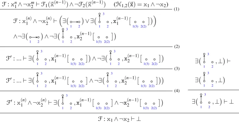
For this subsection, we have opted for a new minimal example without the blowup from the weakest liberal precondition in Subsection 3.3. The example (Fig. 9) uses a minimal number of variables to show the calculusKµ and its inductive refutation rule at work. We examine the µ-conditionx1∧ ¬x2, whose main body has type
1 2
. Consider the following systemF:
x1 1 2 =∃ 1 2 ∨ ∃ 1 2 3 ,x1 1(3) 2(2)
; x2 1 2 =∃ 1 2 ∨ ∃ 1 2 3 ,x2 1(3) 2(2)
While the equations are syntactically identical up to variable renaming, this is not exploited by
Kµ, hence the proof is not a one-liner: it starts by defining a suitable list of auxiliary conditions
F:xn1∧ ¬xm2 `F1(~x(n−1))∧ ¬F2(~x(n−1)) (H1,2(~x) =x1∧ ¬x2) (1)
F:x(1n)∧ ¬x(2n)`∃ 1 2
∨ ∃
1 2 3
,x(1n−1)
1(3) 2(2) ∧¬∃ 1 2 ∧ ¬∃ 1 2 3
,x(2n−1) 1(3) 2(2)
(2)
F0:...` ∃
1 2 3
,x(1n−1) 1(3) 2(2)
∧ ¬∃
1 2 3
,x(2n−1) 1(3) 2(2)
(3)
F0:...` ∃
1 2 3
,x(1n−1)
1(3) 2(2)
∧ ¬∃ 1 2
3
,x(2n−1)
1(3) 2(2)
(4)
F0:x(n)
1 ∧ ¬x
(n)
2 ` ∃
1 2 3
,x(1n−1)
1(3) 2(2)
∧ ¬x(2n−1)
1(3) 2(2) ∃ 1 2 3 ,⊥ ` ∃ 1 2 3 ,⊥ ∃ 1 2 3 ,⊥ ` ⊥
F:x1∧ ¬x2` ⊥
~
H(in this case actually a single one, which we nameH1,29), unrolling both variables once (1), then uses distributivity of conjunction over disjunction to resolve the base case of the right hand side ofx1(2), then shifts the other branch ofx2over the corresponding branch ofx1. In a lift and shift step (3), a conjunction of two subconditions is obtained (depending on whether the nodes
3are identified). In step (4), one of these is dropped and the other is used to obtainx1∧ ¬x2, with lower annotations, as a subcondition. Finally we show that the context of this subcondition (monotonic by virtue of being syntactically positive) has lfp⊥, and applyRule EMPTY.
5
Related Work
A summary overview of graph conditions for non-local properties is attempted below (a proof calculus is presented in [PP14] but completeness of a proof calculus has only recently been obtained by Lambers and Orejas [LO14] for nested conditions and remains to be researched for the other approaches). Note that while HR∗ conditions are known to properly contain the monadic second-order definable properties [Rad13] and nested conditions are a special case of each of the other three, we have not yet been able to separateµ-conditions from MSO or HR∗:
reference [Pen09] (here) [Rad13] [PP14]
conditions Nested µ- HR∗
MSO-wlp yes yes incomplete10 yes
theorem prover yes future work
complete proof calculus yes future work
Recently, Poskitt and Plump [PP14] have presented a weakest precondition calculus for an-other extension of nested conditions (monadic second-order conditions) and demonstrated its use in a Hoare logic. The method is arguably closer to reasoning directly in a logic and less graph condition like, but seems successful at solving some of the same problems in a different way. HR∗ conditions [Rad13] are another approach towards the same goal; they have already been mentioned in the main text; there is an ongoing effort at extending the weakest precondition calculus to a subclass including path expressions. Strecker et al. [Str08,PST13] have performed verification of graph transformation system within general-purpose theorem proving environ-ments, with positive path conditions. Dyck and Giese [DG15] automatically check certain kinds of inductive invariants of graph transformation systems. Verification of graph transformation systems via abstract model checking, as opposed to the prover-based approach, can be found in Gadducci et al., Baldan et al., König et al., Rensink et al. [GHK98,BKK03,KK06,RD06].
6
Conclusion and Outlook
We have introduced µ-conditions and achieved a weakest liberal precondition transformation
(Th. 2) and a sound proof calculus (Th. 3) for correctness relative toµ-conditions, which seems
a fruitful ground for further investigations. In analogy to the equivalence between first-order
graph logic and nested graph conditions, we conjecture thatµ-conditions have the same
expres-sivity as fixed point extensions to first-order logic on finite graphs. Also, the expresexpres-sivity of HR∗ conditions [Rad13] or MSO likely differs fromµ-conditions, but this remains to be examined. As the examples show, our weakest precondition calculus (still a research question for HR∗ con-ditions [Rad13] but readily available by logical means in the MSO-conditions formalism [PP14]) produces unwieldy expressions due to partial shift. The blowup is exponential in the interface size (a related blowup is inherited from the weakest precondition calculus of [Pen09]). We can heuristically simplify the expressions and hope that many cases can be resolved automatically.
Future work includes more proof theory and tool support with special attention to semi-auto-mated reasoning, based on the reasoning engine ENFORCEimplemented in [Pen09]. To extend the wlp construction to programs with iteration, one would have to provide (or have the prover attempt to find) an invariant, as in the original work of Pennemann; for termination, one could proceed as in [Pos13] and prove termination variants. It appears thatµ-conditions might readily
generalise to temporal properties, even with the option to nest temporal operators inside quanti-fiers, which would allow properties such as the preservation of a specific node to be expressed (but require further proof rules). This could be achieved via anextoperator parameterised on atomic subprograms (the basic steps ofDef. 3) and since in the semantics of programs the rela-tionship between the interfaces is deterministic, this would again confer an unambiguoustypeto such an expression and make it suitable for use as a subcondition, and allow the expression of eventualities as in the modalµ-calculus[BS07]. Whether this offers any new insights remains to
be seen. We plan to deal with algebraic operations on attributes and extend our work to a verifi-cation method that separates the graph specific concerns from other aspects and allows proofs of properties that depend on both, for example involving data structures with ordered elements.
Acknowledgements: We thank Annegret Habel, many other members of SCARE as well as
several anonymous reviewers for providing valuable criticism of the approach and the text.
Bibliography
[BKK03] P. Baldan, B. König, B. König. A logic for analyzing abstractions of graph transfor-mation systems. InStatic Analysis. Pp. 255–272. Springer, 2003.
[BS07] J. Bradfield, C. Stirling. Modalµ-calculi.Studies in Logic and Practical Reasoning
3:721–756, 2007.
[DG15] J. Dyck, H. Giese. Inductive Invariant Checking with Partial Negative Application Conditions. InICGT. LNCS 9151, pp. 237–253. 2015.
[Dij76] E. W. Dijkstra.A discipline of programming. Prentice Hall, 1976.
[EEPT06] H. Ehrig, K. Ehrig, U. Prange, G. Taentzer.Fundamentals of Algebraic Graph Trans-formation. Monographs in Theoretical Computer Science. Springer, 2006.
[GHK98] F. Gadducci, R. Heckel, M. Koch. A Fully Abstract Model for Graph-Interpreted Temporal Logic. InTAGT’98. LNCS 1764, pp. 310–322. 1998.
[Hoa83] C. A. R. Hoare. An axiomatic basis for computer programming.Communications of the ACM26(1):53–56, 1983.
[HP09] A. Habel, K.-H. Pennemann. Correctness of High-Level Transformation Systems Relative to Nested Conditions.Math. Struct. in Comp. Sci.19(2):245–296, 2009.
[HPR06] A. Habel, K.-H. Pennemann, A. Rensink. Weakest Preconditions for High-Level Programs. InICGT 2006. LNCS 4178, pp. 445–460. 2006.
[KK06] B. König, V. Kozioura. Counterexample-Guided Abstraction Refinement for the Analysis of Graph Transformation Systems. LNCS 3920, pp. 197–211. 2006.
[Kre02] S. Kreutzer.Pure and Applied Fixed-Point Logics. PhD thesis, Dissertation thesis, RWTH Aachen, 2002.
[LO14] L. Lambers, F. Orejas. Tableau-Based Reasoning for Graph Properties. In Graph Transformation. LNCS 8571, pp. 17–32. 2014.
[Pen09] K.-H. Pennemann. Development of Correct Graph Transformation Systems. PhD thesis, Universität Oldenburg, 2009.
[Pos13] C. M. Poskitt.Verification of Graph Programs. PhD thesis, University of York, 2013.
[PP13] C. M. Poskitt, D. Plump. Verifying Total Correctness of Graph Programs.Electronic Communications of the EASST 61, 2013.
[PP14] C. M. Poskitt, D. Plump. Verifying Monadic Second-Order Properties of Graph Pro-grams. InGraph Transformation. LNCS 8571, pp. 33–48. 2014.
[PST13] C. Percebois, M. Strecker, H. N. Tran. Rule-Level Verification of Graph Transforma-tions for Invariants Based on Edges’ Transitive Closure. InSEFM 2013. LNCS 8137, pp. 106–121. 2013.
[RAB+15] H. Radke, T. Arendt, J. Becker, A. Habel, G. Taentzer. Translating Essential OCL Invariants to Nested Graph Constraints Focusing on Set Operations. InProc. ICGT. LNCS 9151, pp. 155–170. 2015.
[Rad13] H. Radke. HR* Graph Conditions Between Counting Monadic Second-Order and Second-Order Graph Formulas.Electronic Communications of the EASST61, 2013.
[RD06] A. Rensink, D. Distefano. Abstract graph transformation.ENTCS157:39–59, 2006.
[Str08] M. Strecker. Modeling and Verifying Graph Transformations in Proof Assistants.
ENTCS203(1):135–148, 2008.
[Tar55] A. Tarski. A lattice-theoretical fixpoint theorem and its applications.Pacific J. Math.