ASIAN JOURNAL OF MATHEMATICS AND APPLICATIONS Volume 2013, Article ID ama0055, 36 pages
ISSN 2307-7743 http://scienceasia.asia
INTEGRAL TRANSFORMS OF THE HARMONIC SAWTOOTH MAP, THE RIEMANN ZETA FUNCTION, FRACTAL STRINGS, AND A FINITE
REFLECTION FORMULA
STEPHEN CROWLEY
Abstract. The harmonic sawtooth map w(x) of the unit interval onto itself is defined. It is shown that its fixed points{x:w(x) =x}are enumerated by then-th derivatives of a Meijer-G function and Lerch transcendent, serving as exponential and ordinary generating functions respectively, and involving the golden ratio in their parameters. The appropriately scaled Mellin transform ofw(x) is an analytic continuation of the Riemann zeta functionζ(s) valid∀−Re(s)̸∈
N. The series expansion of the inverse scaling function associated to the Mellin transform ofw(x) has coefficients enumerating the Large Schr¨oder NumbersSn, defined as the number of perfect matchings in a triangular grid ofnsquares and expressible as a hypergeometric function. A finite-sum approximation toζ(s) denoted byζw(N;s) is examined and an associated functionχ(N;s) is found which solves the reflection formulaζw(N; 1−s) =χ(N;s)ζw(N;s). The functionχ(N;s) is singular ats= 0 and the residue at this point changes sign from negative to positive between the values ofN = 176 and N = 177. Some rather elegant graphs of the reflection functions χ(N;s) are also provided. The Mellin and Laplace transforms of the individual component functions of the infinite sums and their roots are compared. The Gauss maph(x) is recalled so that its fixed points and Mellin transform can be contrasted to those ofw(x). The geometric
counting functionNLw(x) =
⌊√
2x+1
2 −
1 2 ⌋
of the fractal string Lw associated to the lengths of the harmonic sawtooth map components{wn(x)}∞n=1happens to coincide with the counting function for the number of Pythagorean triangles of the form{(a, b, b+ 1) : (b+ 1)6x}. The volume of the inner tubular neighborhood of the boundary of the map∂Lwwith radiusεis shown
to have the particuarly simple closed-formVLw(ε) =4εv(ε)22−v(4εεv)(ε)+1wherev(ε) =
⌊
ε+√ε2+ε 2ε
⌋
.
Also, the Minkowski content ofLwis shown to beMLw= 2 and the Minkowski dimension to be DLw =12 and thus not invertible. The geometric zeta function, which is the Mellin transform of the geometric counting functionNLw(x), is calculated and shown to have a rather unusual closed form involving a finite sum of Riemann zeta functions and binomioal coefficients. Some definitions from the theory of fractal strings and membranes are also recalled.
Contents
1. Unit Interval Mappings 2
1.1. Then-th Harmonic Sawtooth Functionwn(x) 2
1.2. Integrals Transforms of w(x) 4
1.3. The Gauss Map h(x) 15
1.4. The Harmonic Sawtooth Map w(x) as an Ordinary Fractal String 17
2. Fractal Strings and Dynamical Zeta Functions 24
2010Mathematics Subject Classification. 14G10.
Key words and phrases. Integral Transforms; Harmonic Sawtooth Map; Riemann Zeta Function.
c
⃝2013 Science Asia
2.1. Fractal Strings 24
2.2. Fractal Membranes and Spectral Partitions 28
3. Special Functions, Definitions, and Conventions 28
3.1. Special Functions 28
3.2. Applications of w(x) 33
3.3. Conventions and Symbols 34
References 34
1. Unit Interval Mappings
1.1. The n-th Harmonic Sawtooth Function wn(x).
1.1.1. Infinite Sum Decomposition. Let then-th componentwn(x)∈[0,1]∀x∈[0,1] of the harmonic
sawtooth functionw(x) [9, 2.3] be defined as
(1) wn(x) =n(xn+x−1)χ
( x, IH
n
)
where
(2) χ(x, InH)=
{
1 1
n+ 1 < x6 1
n
0 otherwise
is the characteristic function of the n-th harmonic interval(132). By settingn=⌊x−1⌋as in (134)
we get the unit interval mapping
(3)
w(x) =w⌊x−1⌋(x)
=⌊x−1⌋(x⌊x−1⌋+x−1)χ(x, IH
⌊x−1⌋
)
=∑∞n=1wn(x)
=∑∞n=1n(xn+x−1)χ(x, InH)
=⌊x−1⌋ (x⌊x−1⌋+x−1) =x⌊x−1⌋2+x⌊x−1⌋−⌊x−1⌋
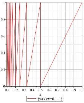
As can be seen in Figure 1,w(x) is discontinuous at a countably infinite set of points of Lebesgue measure zero
(4) H =
{
y: limx→y−w(x)̸= limx→y+w(x)
}
={0,n1 :n∈Z}
The left and right limits at the discontinuous points are
(5) limx→∈H−w(x) = 1
limx→∈H+w(x) = 0
1.1.2. The Fixed Points ofw(x)as an Iterated Function System. The iterates of the map
(6) [w(x), w(w(x)), w(w(w(x))), w(w(w(w(x)))), . . .] =
[
w1(x), w2(x), w3(x), w4(x), . . . ]
have the form
INTEGRAL TRANSFORMS 3
Figure 1. The Harmonic Sawtooth map
where {ar, br∈Z:r∈N}is a pair of integer sequences andc∈Ris some constant. The sequence
of quotients ar
br converges rather quickly to the fixed value
(8) limr→∞abr
r =x−c ∀x∈[0,1]
The explicit equation(sometimes called Schr¨oder’s equation) for the fixed points ofw(x), is
(9)
Fixnw ={x:wn(x) =x}
={x:n(xn+x−1)χ(x, InH) =x}
={x:n(xn+x−1) =x}
= limx→0
d
dxnFixw(x)
n!
= limx→0x
1−n
n! G 1,4 4,4
(
−x| −1 −1 −ϕ ϕ−1
0 n−1 2−ϕ −1−ϕ )
= n
whereGis the Meijer-G function and Fixw(x) is the generation function
(10)
Fixw(x) =
∑∞
n=1 Fix
n wxn
=∑∞n=1n2nx+nn−1
=101 ((5−√5)Φ (x,1,1−ϕ) + (5−√5)Φ (x,1, ϕ))
where Φ(z, a, v) is the Lerch Transcendent (159), and ϕ is the Golden Ratio, which is the ratio of two numbers having the property that the ratio of the sum to the larger equals the ratio of the larger to the smaller. [7, Ch.XX][35, I.7][16, p.50][28] The number ϕ can be called the “most irrational number” because its continued fraction expansion, given by iterations of the Gauss map (78), converges more slowly than any other number. The constant ϕsatisfies the simple identities
(11) ϕ= 1
ϕ−1 =
ϕ ϕ+ 1
(12) ϕ2−ϕ−1 = 0
An interesting fact is that the density of a motif in a certain noncommutative space described in [23, 5.1] must necessarily be an element of the group Z+ϕZ.
1.2. Integrals Transforms of w(x).
1.2.1. Dirichlet Polynomial Series and the Mellin Transform of w(x). The Mellin transform of the harmonic saw mapw(x), multiplied by
(13) τ(s) =ss+ 1
s−1
is an analytic continuation of the Riemann zeta function ζ(s)∀ −Re(s) ̸∈ N. This form of the zeta function, denoted byζw(s), is the infinite sum of the Mellin transformations of the component
functions.
(14)
M[wn(x);x→s] =
∫ 1
n
1
n+1
wn(x)xs−1dx
=∫nn+1wn(x−1)x−s−1dx
=∫01n(xn+x−1)χ(x, IH
n)xs−1dx
=∫
1
n
1
n+1
n(xn+x−1)xs−1dx
=−eln(n)(1−s)−ne sln(n1+1)
−sesln( 1
n)
s2+s
=nnsssn(+ns+1)(n+1)s+ns−ss(2n(n+1)+1)sns
=−n1−s−n(ns2+1)+s−s−sn−s
There is a conjugate pair of inverse branches ofτ(s) found by solving
(15)
τ±−1(t) ={s:τ(s) =t}
=
{
s:sss+1−1 =t }
=2t−12±√1−26t+t2
INTEGRAL TRANSFORMS 5
number of perfect matchings in a triangular grid of n squares, named after Ernst Schr¨ oder(1841-1902).[17, A006318][4, p.340][10]
(16) Sn =2F1
(
n+ 1 2−n
2 | −1
)
2
wherepFq is a hypergeometric function. We have
(17)
limt→0
dn dtnτ−
1 + (t)
n! =
0 n= 0
−1 n= 1 −Sn n>2
limt→0
dn dtnτ
−1
− (t)
n! =
−1 n= 0
2 n= 1
Sn n>2
(18)
n 0 1 2 3 4 5 6 7 8 9 10 11 12 13 14
Sn 1 1 2 6 22 90 394 1806 8558 41586 206098 1037718 5293446 27297738 142078746
The residue at the singular points= 1 of τ(s) is
(19)
Res
s=1(τ(s)M[wn(x);x→s]) = Ress=1 (
s2+s s−1
(
−n1−s−n(n+1)−s−sn−s
s2+s
))
= Res
s=1 (
n(n+1)−s−n1−s+sn−s
s−1
)
= 2∫n1
1
n+1
wn(x)dx
= 2∫
1
n
1
n+1
n(xn+x−1)dx
= 1
n2+n
The infinite sum of the Mellin transforms multiplied byτ(s) analytically continuesζ(s)∀(−Re(s))̸∈N
(20)
ζw(s) =ζ(s)
=τ(s)M[w(x);x→s] =τ(s)∫01w(x)xs−1dx
=sss+1−1∫01⌊x−1⌋ (x⌊x−1⌋+x−1)xs−1dx
=sss+1−1∑∞n=1M[wn(x);x→s]
=sss+1−1∑∞n=1∫n1
1
n+1
n(xn+x−1)xs−1dx
=∑∞n=1ss+1
s−1 (
−n1−s−n(n+1)−s−sn−s
s(s+1)
)
=∑∞n=1n(n+1)−ss−−n11−s+sn−s
= s−11∑∞n=1n(n+ 1)−s−n1−s+sn−s
Unlike the Mellin transform of the Gauss map (78), which must be multiplied by the factorsthen subtracted from s−s1 before it equalsζ(s), the “harmonic sawtooth continuation”ζw(s) of the zeta
functionζ(s) has the fortuitous property that it equals ζ(s) after multiplyingM[w(x);x→s] by
substition∞ →N is made in the infinite sum appearing the expression forζw(s) to get
(21)
ζw(N;s) =τ(s)
∑N
n=1M[wn(x);x→s]
=s−11∑Nn=1n(n+ 1)−s−n1−s+sn−s
= 1
s−1 (
s+ (N+ 1)1−s−1 +s∑N n=2n−
s−∑N+1
n=2 n−
s)
=(s−1)(NN+1)s −
cos(πs)Ψ(s−1,N+1)
Γ(s) +ζ(s)∀s∈N∗
with equality in the limit except at the negative integers
(22) limN→∞ζw(N;s) =ζ(s)∀ −s̸∈N∗
The functionsζw(N;s) have real roots ats= 0 ands=−1. That is
(23) lim
s→0ζw(N;s) = lims→−1ζw(N;s) = 0
The residue ofζw(N;s) ats= 1 is given by
(24)
Res
s=1(ζw(N;s)) = Ress=1 (
τ(s)∑Nn=1M[wn(x);x→s]
)
=∑Nn=1Res
s=1 (
τ(s)M[wn(x);x→s]
)
=∑Nn=1 1
n2+n
=NN+1
Thus, as required
(25)
limN→∞Res
s=1(ζw(N;s)) = limN→∞ ∑N
n=1 1
n2+n
= limN→∞NN+1
= 1
The functionτ(s) has zeros at−1 and 0 and a simple pole at s= 1 with residue
(26) Ress=1(τ(s)) = Ress=1
( ss+1
s−1 )
= 2
The Mellin transform ofτ(s) has an interesting Laurent series, convergent on the unit disc, given by
(27)
M[τ(s);s→t] =∫0∞τ(s)st−1ds
=∫0∞sss+1−1st−1ds
=∑∞n=14ζ(2n−2)t2n−3 ∀|t|<1
=−4iπ(
1 2e
iπt+1 2e−
iπt)
eiπt−e−iπt =−2πcos(sin(πtπt))
The transformations M[wn(x);x→ s] have removable singularities at −1 and 0 where the limits
are given by
(28)
lim
s→−1M[wn(x);x→s] =n
2ln(n+1
n
)
+nln(n+1n )−n
lim
s→0M[wn(x);x→s] = 1 +nln (n+1
n
INTEGRAL TRANSFORMS 7
(29) lims→0e
−M[wn(x);x→s] = (n+ 1)nn−ne−1
lims→−1e−M[wn(x);x→s] =n(n
2+n)
(n+ 1)(−n2−n)en
So, (14) can be rewritten as
(30) M [wn(x);x→s] =
n2ln(n+1n )+nln(n+1n )−n s=−1
1 +nln(n+1n ) s= 0
−n1−s−n(n+1)−s−sn−s
s2+s otherwise
Furthermore, we have the limits
(31)
limn→∞ lim
s→−1M[wn(x);x→s] = limn→∞lims→−1−
n1−s−n(n+1)−s−sn−s s2+s
= limn→∞n2ln
(n+1
n
)
+nln(n+1n )−n
= 12
and
(32)
limn→∞lim
s→0M[wn(x);x→s] = limn→∞lims→0−
n1−s−n(n+1)−s−sn−s s2+s
= limn→∞1 +nln
(n+1
n
)
= 0
The sum of limits overnats=−1 is Euler’s constant. [13][14, 1.1]
(33)
∑∞
n=1
M[wn(x);x→−1]
n =
∑∞
n=1
1+nln(n+1
n )
n
= lims→1ζ(s)−s−11
= limn→∞
∑n k=1
1
k −ln(n)
=γ
∼
= 0.577215664901533. . .
1.2.2. The Reflection Formula for ζw(N;s). There is a reflection equation for the finite-sum
ap-proximation ζw(N;s) which is similiar to the well-known formula ζ(1−s) = χ(s)ζ(s) with
χ(s) = 2 (2π)−scos(πs2)Γ (s). The solution to
(34) ζw(N; 1−s) =χ(N;s)ζw(N;s)
is given by the expression
(35)
χ(N;s) = ζw(N;1−s)
ζw(N;s)
=
∑N n=1−
−ns+(n+1)s−1n+ns−1−ns−1s s
∑N n=1−
n1−s+(n+1)−s n+n−s s s−1
=−(s−1)
∑N n=1−n
s+(n+1)s−1n+ns−1−ns−1s s∑N
n=1−n1−s+(n+1)−sn+n−ss
which satisfies
(36) χ(N; 1−s) =χ(N;s)−1
The functionsχ(N;s), indexed byN, have singularities ats= 0. Let
(37)
a(N) =∑Nn=1n(ln (n+ 1)−ln (n))
b(N) =∑Nn=1ln(n)n2−ln(n(nn+1)+1)n2−ln(n)
c(N) = 12∑Nn=1n (
ln (n+ 1)2−ln (n)2
then the residue at the singular points= 0 is given by the expression (38)
Res
s=0(χ(N;s)) =−Ress=1(χ(N;s)
−1)
=1+γ+Ψ(n+2)−
2
N+1+b(N)−
N(ln(Γ(N+1))−c(N)) (N−a(N))(N+1) a(N)−N
=
1+γ+Ψ(n+2)− 2
N+1+ ∑N
n=1
ln(n)n2−ln(n+1)n2−ln(n)
n(n+1) −
N(ln(Γ(N+1))−1 2
∑N
n=1n(ln(n+1)2−ln(n)2))
(N−∑N
n=1n(ln(n+1)−ln(n)))(N+1)
(∑N
n=1n(ln(n+1)−ln(n)))−N
which has the limit
(39) lim
N→∞Ress=0(χ(N;s)) = 1
We also have the residue of the reciprocal at s= 2
(40) Res
s=2(χ(N;s)
−1) =
2N
(N+1)2−2Ψ(1,N+1)+2ζ(2) (N+1)2
2 −N2−12− ∑N
n=1n(ln(n+1)+ln(n+1)n−ln(n)−nln(n))
which vanishes asN tends to infinity
(41) lim
N→∞Ress=2(χ(N;s)
−1
) = 0
As can be seen in the figures below, the residue at s = 0 changes sign from negative to positive between the values ofN = 176 andN = 177.
Figure 2.
{
Res
INTEGRAL TRANSFORMS 9
Figure 3.
{
Res
s=0(χ(N;s))
−1:N = 1. . .250}
For any positive integer N, we have the limits
(42)
lims→0χ(N;s) =∞
lims→0 d
n
dsnχ(N;s) =∞ lims→1
2χ(N;s) = 1
lims→1χ(N;s) = 0
lims→2χ(N;s) = 0
lims→1ddsχ(N;s) = 0
The line Re (s) = 12 has a constant modulus
(43) χ
( N;1
2+is
) = 1 There is also the complex conjugate symmetry
(44) χ(N;x+iy) =χ(N;x−iy)
Ifs=n∈N∗ is a positive integer thenχ(N;n) can be written as
(45)
χ(N;n) =ζw(N;1−n)
ζw(N;n)
=
∑N m=1−
∑n−2
k=1 mkn ( n−1
k−1)
N
(n−1)(N+1)n−cos(πn)Ψ(Γ(nn)−1,N+1)+ζ(n)
= −
∑N
m=11n((n−1)m
n−1+mn−(m+1)n−1m)
N
(n−1)(N+1)n−cos(πn)Ψ(Γ(nn)−1,N+1)+ζ(n)
The Bernoulli numbers[1] make an appearance since
(46) χ(N; 2n)ζw(N; 2n) =B2n(N+ 1)2 (2 n+1)
The denominator ofχ(N;n) has the limits
(47) limN→∞ζw(N;n) =ζ(n)
limn→∞ζw(N;n) = 1
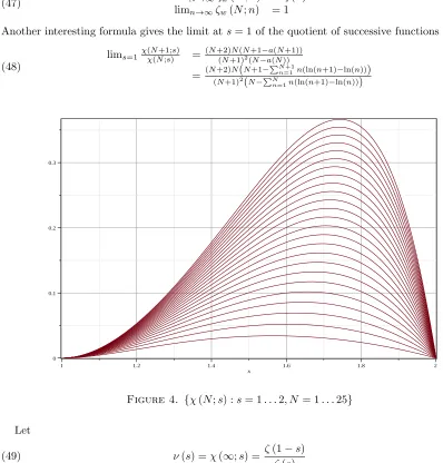
Another interesting formula gives the limit at s= 1 of the quotient of successive functions
(48)
lims=1
χ(N+1;s)
χ(N;s) =
(N+2)N(N+1−a(N+1)) (N+1)2(N−a(N))
= (N+2)N(N+1−
∑N+1
n=1n(ln(n+1)−ln(n)))
(N+1)2(N−∑N
n=1n(ln(n+1)−ln(n)))
Figure 4. {χ(N;s) :s= 1. . .2, N = 1. . .25}
Let
(49) ν(s) =χ(∞;s) = ζ(1−s)
ζ(s)
Then the residue at the even negative integers is
(50) Res
s=−n(ν(s)) =
{ ζ(1−n)
d
dsζ(s)|s=−n neven
0 nodd
1.2.3. The Laplace Transforms L[wn(x);x→ s]. The Laplace transform L[wn(x);x→ s] and its
roots are calculated to shed light on the behaviour roots of the Mellin transformsM[wn(x);x→s]
INTEGRAL TRANSFORMS 11
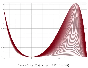
Figure 5. {χ(N;s) :s= 12. . .2, N= 1. . .100 }
function is given by
(51)
L[wn(x);x→s] =
∫1
0 wn(x)e−
xsdx
=∫01n(xn+x−1)χ(x, InH)e−xsdx
=∫
1
n
1
n+1
n(xn+x−1)e−xsdx
= n(n+1)e− s
n+1−(n2+n+s)e−sn s2
There is a removable singularity ats= 0 which has the limit
(52)
L[wn(x);x→0] = lims→0L[wn(x);x→s]
= lims→0n(n+1)e
− s
n+1−(n2+n+s)e−ns
s2
=12Res
s=1(τ(s)M[wn(x);x→s])
= 1
2n(n+1)
Additionally,
(53)
∑∞
n=1L[wn(x);x→0] =
∑∞
n=1lims→0
n(n+1)e−ns+1−(n2+n+s)e−ns s2
=∑∞n=1 1 2n(n+1)
= limn→∞ lim
s→−1M[wn(x);x→s]
= limn→∞lims→−1−
n1−s−n(n+1)−s−sn−s
s2+s
The roots ofL[wn(x);x→s] are enumerated by
(54) ρL
wn(m) ={s:L[wn(x);x→s] = 0}=−n(n+ 1)W(m,−e
−1)−n(n+ 1)
whereW(m, x) is the Lambert W function (146) andm∈Z, n∈N. It can be verified that
(55) L[wn(z);x→ρLwn(m)] =
e(n+1)(1+W(m,−e−1 ))W(m,−e−1)+en(1+W(m,−e−1 )) n(1+W(m,−e−1))2(n+1) = 0
where−e−1 is expressed as the continued fraction via its quotient sequence
(56) −e−1= [−1,1,1,1,2,1,1,4,1,1,6,1,1,8,1,1,10,1,1,12,1,1,14,1,1,16,1,1,18,1,1,20, ...]
The rootsρL
wn(m) satisfy a functional reflection equation with respect to m
(57) ρ
L
wn(m) =ρ
L
wn(−m−1)
−n(n+ 1)W(m,−e−1)−n(n+ 1) =−n(n+ 1)W(−m−1,−e−1)−n(n+ 1)
where ¯x= Re(x)−Im(x) denotes complex conjugation. The quotients of the roots of consecutive transforms is
(58) ρ
L wn(m)
ρL wn−1(m)
= nn+1−1
Thus
(59) limn→∞
ρL wn(m)
ρL wn−1(m)
= limn→∞nn+1−1 = 1
1.2.4. The RootsρMwn(m)of M[wn(x);x→s]. Define
(60) Mτ w(s, n) =τ(s)M[wn(x);x→s] = n(n+1)−ss−−n11−s+sn−s
as in (21) and its infinte number of inverse branches (which are currently lacking closed-form expression if such a thing is possible except whenn= 1), where the branches are indexed bym
(61) M
−1
τ w(z, n, m) ={s:τ(s)M[wn(x);x→s] =z}
=
{
s: n(n+1)−ss−−n11−s+sn−s =z }
then we see that the first function wheren= 1, Mτ w−1(z,1, m), has the closed-form
(62) M−1
τ w(z,1, m) =
W(m,ln(
√
2)
z−1 )
+ln(2)
ln(2)
whereW is the Lambert W function (146). It is verified that
(63) Mτ w(M−1
τ w(z,1, m),1, m) =−
1−2−
W
(
m,ln(
√
2)
z−1
)
+ln(2) ln(2) −W
(
m,ln(
√
2)
z−1
) +ln(2) ln(2) W ( m,ln( √ 2)
z−1
)
+ln(2) ln(2) −1
=z
Furthermore, let ρM
wn(m) denote them-th root ofM[wn(x);x→s]
(64) ρ
M
wn(m) ={s:M[wn(x);x→s] = 0} =M−1
w (0, n, m)
which satisfies
(65) Im(ρM
wn(m)
) >Im
( ρM
wn−1(m)
INTEGRAL TRANSFORMS 13
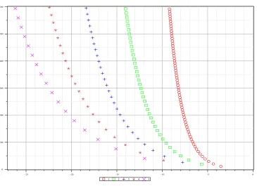
Figure 6. The RootsρLwn(m) of{L[wn(x);x→s] :n∈1. . .9}
(66) limm→±∞Re(ρMwn(m)) = 0
Thus,
(67) limm→±∞arg
(
ρMwn(m)) =π2
1.2.5. Quotients and Differences ofρMwn(m). Let
(68) ∆ρM
wn(m) =ρ
M
wn(m+ 1)−ρ
M wn(m)
be the forward difference of consecutive roots ofM[wn(x);x→s]. The limiting difference between
by
(69)
∆ρMwn(±∞) = limm→±∞∆ρMwn(m) ={s:ns2 + (n+ 1)s2 = 0}
= limm→±∞
( ρM
wn(m+ 1)−ρ
M wn(m)
)
= limm→±∞
(
ρMwn(m)
m
)
=M[χ(x,I2πiH n);x→0]
= 2πi
lims→0 (
n−s−(n+1)−s
s
)
=ln(n+1)2πi−ln(n)
LetQ∞ρM wn
denote the limit
(70)
Q∞
ρM
wn = limm→±∞
ρMwn(m)
ρM wn−1(m)
= ∆ρ M wn(±∞)
∆ρM wn−1(±∞)
= M[χ(x,(
1
n+1, 1
n));x→0]
M[χ(x,(1
n,
1
n−1));x→0]
= ln(ln(nn)+1)−ln(−nln(−n1))
then we also have the limit of the limitsQ∞ρM wn
as n→ ∞given by
(71)
limn→±∞Q∞ρM
wn = limn→±∞
(
∆ρMwn(±∞) ∆ρM
wn−1(±∞)
)
= limn→±∞
( ln(n)−ln(n−1)
ln(n+1)−ln(n) ln(n−1)−ln(n−2)
ln(n)−ln(n−2)
)
= limn→±∞
(
ln(n)−ln(n−1) ln(n+1)−ln(n) )
= 1
The limiting quotients e−ρMwn(m+1)
e−ρMwn(m) =e
ρMwn(m)−ρMwn(m+1)asm→ ∞are given by
(72)
limm→∞eρ
M
wn(m)−ρMwn(m+1) = 1−2 sin
(
π
ln(n+1)−ln(n) )2
−2icos
(
π
ln(n+1)−ln(n) )
sin
(
π
ln(n+1)−ln(n) )
=e−ln(n+1)2πi−ln(n)
where we have
(73)
|limm→∞eρ
M
wn(m)−ρMwn(m+1)| = limm→∞|eρMwn(m)−ρMwn(m+1)|
=
√
e−ln(n+1)2πi−ln(n)
= 1
and
(74) limn→∞limm→∞eρ
M
INTEGRAL TRANSFORMS 15
Figure 7. {ρMwn(m) :m= 1. . .5}
1.2.6. The Laplace Transform L[(s−1)M[wn(x);x→s] ;s → t]. The Laplace transform of (s−
1)M[wn(x);x→s] defined by
(75)
L[(s−1)M[wn(x);x→s] ;s→t] =L[n(n+ 1)−s+sn−s−n1−s;s→t]
=∫0∞n(n+ 1)−s+sn−s−n1−se−stds
= t+ln( nn
(n+1)n)t+ln(n+1)+nln(n)2−nln(n) ln(n+1)
(ln(n)+t)2(ln(n+1)+t)
has poles at−ln(n) and−ln(n+ 1) with residues
(76)
Res
t=−ln(n) (
L[(s−1)M[wn(x);x→s];s→t]
)
=−n
Res
t=−ln(n+1) (
L[(s−1)M[wn(x);x→s];s→t]
)
=n
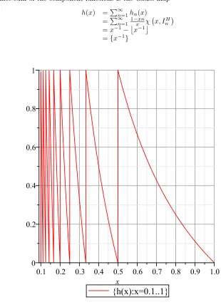
1.3. The Gauss Map h(x).
1.3.1. Continued Fractions. The Gauss maph(x), also known as the Gauss function or Gauss trans-formation, maps unit intervals onto unit intervals and by iteration gives the continued fraction expansion of a real number [38, A.1.7][35, I.1][12, X] The n-th component function hn(x) of the
maph(x) is given by
(77) hn(x) =1−xxnχ
The infinite sum of the component functions is the Gauss map
(78)
h(x) =∑∞n=1hn(x)
=∑∞n=11−xxnχ(x, InH
)
=x−1−⌊x−1⌋
={x−1}
Figure 8. The Gauss Map
The fixed points ofh(x) are the (positive) solutions to the equationhn(x) =xgiven by
(79)
Fixnh ={x:hn(x) =x}
={x: 1−xxnχ(x, InH)=x}
={x: 1−xn
x =x
}
= √n22+4−n
INTEGRAL TRANSFORMS 17
1.3.2. The Mellin Transform ofh(x). The Mellin transform (138) of the Gauss maph(x) over the unit interval, scaled bysthen subtracted from s−s1, is an analytic continuation ofζ(s), denoted by
ζh(s), valid for all−Re(s))̸∈N. The transfer operator and thermodynamic aspects of the Gauss
map are discussed in [42][41][40][39][36]. The Mellin transform of the n-th component function
wn(x) is given by
(80)
M[hn(x);x→s] =
∫1 0 hn(x)x
s−1dx
=∫011−xxnχ(x, InH)xs−1dx
=∫ 1 n 1 n+1 (
x−1−⌊x−1⌋)xs−1dx
=∫n1
1
n+1
1−xn
x x
s−1dx
=−n(n+1)−s+ss2(n−+1)s −s−n1−s
which provides an analytic continuationζh(s) =ζ(s)∀(−Re(s))̸∈N
(81)
ζh(s) =s−s1−sM[h(x);x→s]
=s−s1−s∫01h(x)xs−1dx
=s−s1−s∫01(x−1−⌊x−1⌋)xs−1dx
= s
s−1−s ∑∞
n=1M[hn(x);x→s]
= s
s−1− 1
s−1 ∑∞
n=1−(n(n+ 1)−
s+s(n+ 1)−s−n1−s)
=s−s1−s−11∑∞n=1n1−s−n(n+ 1)−s−s(n+ 1)−s
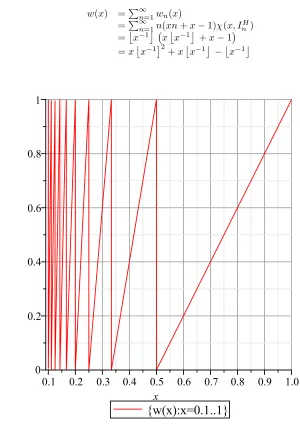
1.4. The Harmonic Sawtooth Map w(x) as an Ordinary Fractal String.
1.4.1. Definition and Length. Let
(82) InH =
( 1
n+1, 1
n
)
be the n-th harmonic interval, then{w(x)∈ Lw : x∈ Ω} is the piecewise monotone mapping of
the unit interval onto itself. The fractal string Lw associated with w(x) is the set of connected
component functions wn(x) ⊂ w(x) where each wn(x) mapsInH onto (0,1) and vanishes when
x̸∈InH. Thus, the disjoint union of the connected components of Lw is the infinite sum w(x) =
∑∞
n=1wn(x) where only 1 of thewn(x) is nonzero for eachx, thusw(x) maps entire unit interval onto
itself uniqely except except for the points of discontinuity on the boundary∂Lw={0,n1 :n∈N∗}
where a choice is to be made between 0 and 1 depending on the direction in which the limit is approached. Let
(83) wn(x) =n(xn+x−1)χ(x, InH)
whereχ(x, IH
n ) is then-th harmonic interval indicator (127)
(84) χ(x, IH
n ) =θ
(
xn+x−1
n+1 )
−θ(xn−1
n
)
The substitutionn→⌊x1⌋can be made in (132) where it is seen that
(85) χ
(
x, I⌊Hx−1⌋
)
=θ (x⌊
x−1⌋+x−1 ⌊
x−1⌋+1
)
−θ (
x⌊x−1⌋−1
⌊x−1⌋
)
and so making the same substitution in (83) gives
(86)
w(x) =∑∞n=1wn(x)
=∑∞n=1n(xn+x−1)χ(x, IH n )
=⌊x−1⌋ (x⌊x−1⌋ +x−1)
=x⌊x−1]2+x⌊x−1⌋ −⌊x−1⌋
Figure 9. The Harmonic Sawtooth Map
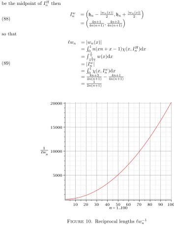
The intervals Iw
n will be defined such thatℓwn=|Inw|=|wn(x)|. Let
(87)
hn =
∫
IH n
x(n+ 1)ndx
=(
1
n+1+n1)
2
INTEGRAL TRANSFORMS 19
be the midpoint ofIH n then
(88) I
w
n =
( hn−|
wn(x)|
2 ,hn+
|wn(x)|
2 )
=
( 4n+1 4n(n+1),
4n+3 4n(n+1)
)
so that
(89)
ℓwn =|wn(x)|
=∫01n(xn+x−1)χ(x, IH n)dx
=∫
1
n
1
n+1
w(x)dx
=|Iw n|
=∫01χ(x, Inw)dx
= 4n4(nn+3+1)−4n4(nn+1+1) = 2n(n1+1)
Figure 10. Reciprocal lengthsℓwn−1
The total length ofLw is
(90)
|Lw| =
∫1
0 w(x)dx
=∑∞n=1ℓwn
=∑∞n=1 1 2n(n+1)
Figure 11. χ(x, Inw) green andwn(x) blue forn= 1. . .3 andx=14..1
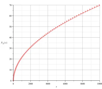
1.4.2. Geometry and Volume of the Inner Tubular Neighborhood. The geometric counting function (109) ofLwis
(91)
NLw(x) = #{n>1 :ℓw−1
n 6x}
= #{n>1 : 2(n+ 1)n6x}
=
⌊√
2x+1
2 −
1 2 ⌋
which is used to calculate the limiting constant (111)Cwappearing in the equation for the
Minkows-ki content
(92)
Cw = limx→∞ NLw(x)
xDLw = limx→∞
√
2x+1 2√ −12
x
= √2 2
The function NLw(x) happens to coincide with [17, A095861], which is the number of primitive Pythagorean triangles of the form{(a, b, b+ 1) : (b+ 1)6n}. [6, 171-176][37, 10.1][18, 11.2-11.5] Let
(93) v(ε) = min(j:ℓwj<2ε) =
⌊
ε+√ε2+ε
2ε
INTEGRAL TRANSFORMS 21
which is the floor of the solution to the inverse length equation
(94)
ε+√ε2+ε
2ε ={n:ℓwn−1= 2ε}=
{ n: 1
2n(n−1) = 2ε }
ℓw
ε+√ε2 +ε
2ε −1
2 =ε
Then the volume of the inner tubular neighborhood of∂Lwwith radiusε(108) is
(95)
VLw(ε) = 2εNLw(21ε)+∑ℓwj<2ε
j ℓwj
= 2εNLw(1 2ε
)
+∑∞n=v(ε) 1 2(n+1)n
= 2εNLw(21ε)+2v1(ε)
= 2ε ⌊√1
ε+1 2 − 1 2 ⌋ + 1
2v(ε)
=4εv(ε)22−v(4εεv)(ε)+1
since
(96) ∑∞n=m
1 2n(n+1) =
1 2m
and by defintion we have
(97) limε→0+VLw(ε) = 0
limε→∞VLw(ε) =|Lw|=
1 2
Thus, using (92) and (95), the Minkowski content (110) ofLw is
(98)
MLw = lime→0+
VLw(ε)
ε1−DLw
= lime→0+ √1 ε
(
2ε ⌊√1
ε+1
2 −
1 2 ⌋
+12
⌊
ε+√ε2+ε
2ε
⌋−1)
= Cw21−DLw
1−DLw
= √
2 2 2
1−1 2
1−1 2
= 2
1.4.3. The Geometric Zeta Function ζLw(s). The geometric zeta function (112) of w(x) is the Dirichlet series of the lengths ℓwn (89) and also an integral over the geometric length counting
function (91)NLw(x)
(99)
ζLw(s) =∑∞n=1ℓws j
=∑∞n=1
( 1 2n(n+1)
)s
=∑∞n=12−s(n+ 1)−sn−s
=s∫0∞NLw(x)x−s−1dx
=s∫0∞ ⌊√
2x+1
2 −
1 2 ⌋
Figure 12. Geometric Counting FunctionNLw(x) ofw(x)
The residue (115) ofζLw(s) atDLw is
(100)
Res(ζL(s))
s=DL
= lims→D+
Lw
(s−DL)ζL(s)
= lims→1 2 +
(
s−12)ζL(s) = lims→1
2 +
(
s−12) ∑∞n=12−s(n+ 1)−sn−s
= lims→1 2 +
(
s−12)s∫0∞ ⌊√2x+1
2 −
1 2 ⌋
x−s−1dx
= 0
The values ofζLw(n) at positive integer valuesn∈N∗are given explicitly by a rather unwieldy sum of binomial coefficients and the Riemann zeta functionζ(n) at even integer values. First, define
(101)
an =
(n−1)(1−(−1)n+1)
2 bn =
(−1)n+1(n−1)
2 +n−
7 4+
(−1)n
4 cn = (−1)n(n−1)
dn =(−1)
n
2
INTEGRAL TRANSFORMS 23
Figure 13. {v(ε) = min(n:ℓwn <2ε) :ε= 10001 . . .14}
(102) ζ
Lw(n) =
(−1)n(2n−1
n−1)
2n +
∑bn
m=an
2(−1)n(2m+cn−dn+ 12
n−1 )ζ(dn+2n− 3
2−2m−cn)
2n
The terms ofζLw(n) fromn= 1 to 10 are shown below in Table 1.
+1 2 −3 4 + 1 2ζ(2)
+5
3 −
3 4ζ(2)
−35
16 +
5
4ζ(2) + 1 8ζ(4)
+63
16 −
35
16ζ(2) − 5 16ζ(4)
−231
32 +
63
16ζ(2) + 21
32ζ(4) + 1 32ζ(6)
+429
32 −
231
32 ζ(2) − 21
16ζ(4) − 7 64ζ(6)
−6435
256 +
429
32 ζ(2) + 165
64 ζ(4) + 9
32ζ(6) + 1 128ζ(8)
+12155 256 −
6435
256 ζ(2) − 1287
256 ζ(4) − 165
256ζ(6) − 9 256ζ(8)
−46189 512 +
12155
256 ζ(2) + 5005
512 ζ(4) + 715
512ζ(6) + 55
512ζ(8) + 1 512 ζ(10)
Figure 14. Volume of the inner tubular neighborhood of∂Lw with radiusε
{
VLw(ε) :ε= 0. . .18}
2. Fractal Strings and Dynamical Zeta Functions
2.1. Fractal Strings. A a fractal stringL is defined as a nonempty bounded open subset of the real line L ⊆Rconsisting of a countable disjoint union of open intervalsIj
(103) L=
∞
∪
j=1 Ij
The length of thej-th intervalIj is denoted by
(104) ℓj=|Ij|
where | ·|is the 1-dimensional Lebesgue measure. The lengthsℓj must form a nonnegative
monot-ically decreasing sequence and the total length must be finite, that is
(105) |L|1=
∑∞
j=1ℓj<∞
ℓ1>ℓ2>. . .>ℓj>ℓj+1>· · ·>0
The case whenℓj= 0 for anyjwill be excluded here sinceℓj is a finite sequence. The fractal string
is defined completely by its sequence of lengths so it can be denoted
INTEGRAL TRANSFORMS 25
Figure 15.
{
VL√w(ε)
ε :ε= 0. . .
1 8 }
and VL√w(8−1)
8−1 =
√ 2
The boundary of L in R, denoted by ∂L ⊂ Ω, is a totally disconnected bounded perfect subset which can be represented as a string of finite length, and generally any compact subset of Ralso has this property. The boundary ∂L is said to be perfect since it is closed and each of its points is a limit point. Since the Cantor-Bendixon lemma states that there exists a perfect set P ⊂∂L
such that∂L −P is a most countable, we can defineLas the complenent of∂Lin its closed convex hull. The connected components of the bounded open setL\∂L are the intervalsIj. [25, 1.2][32,
2.2 Ex17][23, 3.1][30][21][20][15][22][11][19][29]
2.1.1. The Minkowski Dimension DL and Content ML. The Minkowski dimension DL ∈ [0,1], also known as the box dimension, is maximum value ofV(ε)
(107) DL = inf{α>0 :V(ε) =O(ε1−α) asε→0+}=ζ
whereV(ε) is the volume of the inner tubular neighborhoods of∂Lwith radiusε
(108)
VL(ε) =|x∈ L:d(x, ∂L)< ε|
=
ℓj∑>2ε
j
2ε+
ℓj∑<2ε
j
ℓj
= 2εNL (
1 2ε
)
+
ℓj∑<2ε
j
ℓj
andNL(x) is the geometric counting function which is the number of components with their recip-rocal length being less than or equal to x.
(109)
NL(x) = #{j>1 :ℓ−j16x}
=∑ℓ −1
j 6x
j>1 1
The Minkowski content of Lis then defined as
(110)
ML = lime→0+ VL(ε)
ε1−DL = CL21−DL
1−DL
= Res(ζDL(s);DL)21−DL L(1−DL)
whereCL is the constant
(111) CL= limx→∞
NL(x)
xDL
IfML∈(0,∞) exists thenLis said to be Minkowski measurable which necessarily means that the geometry ofL does not oscillate and vice versa. [27, 1] [3][24][26, 6.2]
2.1.2. The Geometric Zeta FunctionζL(s). The geometric Zeta functionζL(s) ofLis the Dirichlet series
(112) ζL(s) =
∑∞
n=1ℓ
s j
=s∫0∞NLw(x)x−s−1dx
which is holomorphic for Re(s)> DL. IfLis Minkowski measurable then 0< DL<1 is the simple unique pole ofζL(s) on the vertical line Re(s) =DL. AssumingζL(s) has a meromorphic extension to a neighboorhood ofDL thenζL(s) has a simple pole atζL(DL) if
(113) NL(s) =O(sDL) ass→ ∞
or if the volume of the tubular neighborhoods satisfies
(114) VL(ε) =O(ε1−DL) asε→0+
It can be possible that the residue ofζL(s) ats=DL is positive and finite
(115) 0< lim
s→DL
(s−DL)ζL(s)<∞
even ifNL(s) is not of ordersDL ass→ ∞andV
INTEGRAL TRANSFORMS 27
2.1.3. Complex Dimensions, Screens and Windows. The set of visible complex dimensions of L, denoted byDL(W), is a discrete subset ofCconsisting of the poles of{ζL(s) :s∈W}.
(116) DL(W) ={w∈W :ζL(w) isapole}
WhenW is the entire complex plane then the setDL(C) =DL is simply called the set of complex dimensions of L. The presence of oscillations in V(ε) implies the presence of imaginary complex dimensions with Re(·) =DL and vice versa. More generally, the complex dimensions of a fractal string Ldescribe its geometric and spectral oscillations.
2.1.4. Frequencies of Fractal Strings and Spectral Zeta Functions. The eigenvaluesλnof the
Dirich-let Laplacian ∆u(x) =−ddx22u(x) on a bounded open set Ω⊂Rcorrespond to the normalized
fre-quenciesfn=
√
λn
π of a fractal string. The frequencies of the unit interval are the natural numbers
n∈N∗and the frequencies of an interval of lengthℓarenℓ−1. The frequencies ofLare the numbers
(117) fk,j =kℓ−j1∀k, j∈N∗
The spectral counting function NvL(x) counts the frequencies ofL with multiplicity
(118) NvL(x) =
∑∞
j=1NL (
x j
)
=∑∞j=1⌊xℓj⌋
The spectral zeta functionζυL(s) ofL is connected to the Riemann zeta function (??) by
(119)
ζυL(s) =
∑∞
k=1 ∑∞
j=1k−
sℓs j
=ζ(s)∑∞n=1ℓs j
=ζ(s)ζL(s)
[27, 1.1][25, 1.2.1]
2.1.5. Generalized Fractal Strings and Dirichlet Integrals. A generalized fractal string is a positive or complex or local measureη(x) on (0,∞) such that
(120)
∫ x0
0
η(x)dx= 0
for some x0 > 0. A local positive measure is a standard positive Borel measure η(J) on (0,∞) whereJ is the set of all bounded subintervals of (0,∞) in which caseη(x) =|η(x)|. More generally, a meausre η(x) is a local complex measure if η(A) is well-defined for any subsetA ⊂[a, b] where [a, b] ⊂ [0,∞] is a bounded subset of the positive half-line (0,∞) and the restriction of η to the Borel subsets of [a, b] is a complex measure on [a, b] in the traditional sense. The geometric counting function ofη(x) is defined as
(121) Nη(x) =
∫x
0 η(x)dx
The dimension Dη is the abscissa of conergence of the Dirichlet integral
(122) ζ|η|(σ) =
∫ ∞
0
x−σ|η(x)|dx
In other terms, it is the smallest real positiveσsuch that the improper Riemann-Lebesgue converges to a finite value. The geometric zeta function is defined as the Mellin transform
(123) ζη(s) =
∫ ∞
0
x−sη(x)dx
2.2. Fractal Membranes and Spectral Partitions.
2.2.1. Complex Dimensions of Dynamical Zeta Functions. The fractal membrane TL associated
withL is the adelic product
(124) TL=
∞
⨿
j=1
Tj
where each Tj is an interval Ij of length log(ℓ−j1)−
1. To each T
j is associated a Hilbert space
Hj =L2(Ij) of square integrable functions on Ij. The spectral partition function ZL(s) of L is a
Euler product expansion which has no zeros or poles in Re(s)> DM(L).
(125) ZL(s) =
∏∞
j=1 1 1−ℓs
j =∏∞j=1ZLj(s)
where DM(L) is the Minkowski dimension of L and ZLj(s) =
1 1−ℓs
j
is the j-th Euler factor, the
partition function of thej-th component of the fractal membrane. [23, 3.2.2]
2.2.2. Dynamical Zeta Functions of Fractal Membranes. The dynamical zeta function of a fractal membraneLis the negative of the logarithmic derivative of the Zeta function associated with L.
(126) ZL(s) =−
d
dsln(ζL(s))
=−ddsζL(s)
ζL(s)
3. Special Functions, Definitions, and Conventions
3.1. Special Functions.
3.1.1. The Interval Indicator (Characteristic) Functionχ(x, I). The (left-open, right-closed) inter-val indicator function is χ(x, I) whereI= (a, b]
(127)
χ(x, I) =
{
1 x∈I
0 x̸∈I
=
{
1 a < x6b
0 otherwise
=θ(x−a)−θ(x−a)θ(x−b)
andθ is the Heaviside unit step function, the derivative of which is the Dirac delta functionδ
(128)
∫
δ(x)dx =θ(x)
θ(x) =
{
0 x <0 1 x>0
The discontinous point ofθ(x) has the limiting values
(129) limx→0−θ(x) = 0
limx→0+θ(x) = 1
thus the values of χ(x,(a, b)) on the boundary can be chosen according to which side the limit is regarded as being approached from.
(130)
limx→a−χ(x,(a, b]) = 0
limx→a+χ(x,(a, b]) = 1−θ(a−b)
INTEGRAL TRANSFORMS 29
3.1.2. “Harmonic” Intervals. Let then-th harmonic (left-open, right-closed) interval be defined as
(131) IH
n =
( 1
n+1, 1
n
]
then its characteristic function is
(132)
χ(x, IH
n) =θ
(
x−n+11 )
−θ(x−n1)
=θ (
x−nn+1 )
−θ(x−n)
=
{
1 n+11 < x6 n1
0 otherwise
As can be seen
(133)
∪∞
n=1I
H n = ∪∞ n=1 ( 1
n+1, 1
n
]
= (0,1]
∑∞
n=1χ(x, I
H
n ) =
∑∞
n=1χ (
x, (
1
n+1, 1
n
])
=χ(x,(0,1])
The substitutionn→⌊x1⌋can be made in (132) where it is seen that
(134) χ
( x, IH
⌊x−1⌋
)
=θ (x⌊
x−1⌋+x−1 ⌊
x−1⌋+1
)
−θ (x⌊
x−1⌋−1
⌊x−1⌋
)
= 1 ∀x∈[−1,+1]
3.1.3. The Laplace TransformLba[f(x);x→s]. The Laplace transform [2, 1.5] is defined as
(135) Lb
a[f(x);x→s] =
∫b af(x)e−
xsdx
where the unilateral Laplace transform is over the interval (a, b) = (0,∞) and the bilateral transform is over (a, b) = (−∞,∞). When (a, b) is not specified, it is assumed to range over the support of
f(x) if the support is an interval. If the support of f(x) is not an interval then (a, b) must be specified. ApplyingLto the interval indicator function (127) gives
(136)
Lba[χ(x,(a, b));x→s] =
∫b
a χ(x,(a, b))e− xsdx
=∫ab(θ(x−a)−θ(x−b)θ(x−a))e−xsdx
=esebsbs−eeasas
=−(eas−ebss)e−s(b+a)
The limit at the singular points= 0 is
(137) lims→0Lba[χ(x,(a, b));x→s] = lims→0−(e
as−ebs)e−s(b+a) s
=b−a
3.1.4. The Mellin TransformMb
a[f(x);x→s]. The Mellin transform [31, 3.2][33, II.10.8][5, 3.6] is
defined as
(138) Mb
a[f(x);x→s] =
∫b af(x)x
s−1dx
![Figure 6. The Roots ρLwn(m) of {L[wn(x); x → s] : n ∈ 1 . . . 9}](https://thumb-us.123doks.com/thumbv2/123dok_us/7822230.2087800/13.612.108.472.95.380/figure-roots-rlwn-m-l-wn-x-x.webp)