STUDY OF AEROSOL OPTICAL DEPTH CLIMATOLOGY
USING MODIS REMOTE SENSING DATA
Amaury de Souza,
[a]*Marcel Carvalho Abreu,
[b]José Francisco de
Oliveira-Júnior,
[c]Cícero Manoel dos Santos,
[d]Ivana Pobocikova,
[e]Widinei A.
Fernandes,
[a]Emmanuel Torsen,
[f]Elania Barros da Silva
[g]and Yohana
Vandi Mbaga
[h]Keywords: Aerosol, satellite, remote sensing, AERONET, MODIS, wildfires.
The temporal variations of the aerosols and their relations with the meteorological conditions in the center of Brazil were studied to understand their interactions with meteorological parameters. Dissimilar cyclical variations are observed due to the trends of the annual cycle: first decreasing and then increasing. Principal component analysis (PCA) may imply the reasons for different characteristics of the temporal variations of the Aerosol Optical Thickness (AOT) and also confirm that their distributions are influenced by complex interactions between different meteorological factors. The average AOT during the selected period has been positively correlated with the thermal and pollutant variables, but negatively correlated with the humid variables.
* Corresponding Authors
E-Mail: [email protected]
[a] Federal University of Mato Grosso do Sul, C.P. 549, 79070- 900. Campo Grande, MS, Brazil
[b] Universidade Federal Rural do Rio de Janeiro, Seropédica, Rio de Janeiro, Brasil
[c] Universidade Federal de Alagoas, Instituto de Ciências Atmosféricas (ICAT), Maceió, Brazil
[d] Federal University of Para, Altamira, PA, Brazil
[e] Department of Applied Mathematics, Faculty of Mechanical Engineering, University of Zilina, Slovakia
[f] Department of Statistics and Operations Research,School of Physical Sciences, Modibbo Adama University of
Technology Yola, Nigeria
[g] Secretaria Municipal de Capela (SMC), Capela , 57780-000 , Alagoas, Brasil
[h] Department of Statistics and Operations Research, School of Physical Sciences, Modibbo Adama University of
Technology Yola, Nigeria
INTRODUCTION
The atmospheric aerosol consists of solid and liquid particles suspended in the atmosphere, studies of its physical characteristics and chemical composition allow anticipating possible climate changes, with ecological and long-term consequences.1,2 Atmospheric aerosols resulting from the
burning of biomass, dust minerals, volcanic ashes, smoke, sea salt, and particulate matters, stand out amongst the various natural and anthropogenic influences. Aerosols are important components of the Earth system3 and decisively influence
global and regional climate change,4,5 air quality,6 human
health,7-11 the fauna, flora and the environment12 through
direct action and indirect radiation forcing, in addition to directly impacting the cloud processes13 and visibility
variation.14 Aerosols have a significant impact on gas
concentration, distribution, and the hydrologic cycle of the greenhouse effect, affecting the physical and chemical processes occurring in the atmosphere.
Aerosol optical thickness (AOT) is the most comprehensive variable for remote assessment of aerosol loading in the atmosphere and is used to reflect its column loading. Recently,
satellite remote sensing and terrestrial observations have become widely used to monitor spatial and temporal distributions of aerosols at both global and local scale.15-17
Satellite instruments such as Moderate Resolution Imaging Spectroradiometer (MODIS) are used to monitor regional and global scale aerosols and provide continuous and long-term coverage of the territory under study.
Aerosols are closely related to a set of meteorological variables: pressure (PRS), average temperature (TEM), relative humidity (RHU), precipitation (PREC), evaporation (EVP), wind speed (WSP), wind direction (WDI), sunshine duration (SSD), and the individual effects of various weather factors on particulate matter (PM) concentrations. The PM concentrations are also very sensitive to temperature, humidity, wind speed, and precipitation.10,18-23
There are few studies on how aerosol distribution depends on the complex effects of these weather factors. In this paper, AOT and all major meteorological factors were investigated together with aerosol meteorology. Aerosol data of MODIS Tier 2 products has been applied to Principal Component Analysis (PCA) to evaluate statistical relationships between seasonal distributions of average AOTs and meteorological factors. PCA is a statistical technique used to reduce the total number of parameters to a more manageable number by grouping linearly correlated observations into a smaller number of variables in PC space.24 In addition, this technique
combines highly correlated observation information into new principal components (PC) variables, which are often uncorrelated with each other. Initially, the spatial distribution and temporal variation of AOT are evaluated for the central part of Brazil for the period from 2002 to 2011. The objective is to link the properties of aerosol distributions to regional weather conditions.
EXPERIMENTAL
spatial resolution is 100 km. These data come from the NASA Giovanni database. AOT is a non-dimensional physical parameter and indicates how much a beam of radiation is attenuated by aerosols as it propagates in a certain layer of the atmosphere containing aerosols.
The daily records of the O3 and CO concentration present
in the atmosphere and the meteorological data during the study period were provided by the Federal University of South Mato Grosso, where the monitoring station is located. The clarity index (Kt), given by Eqn. (1), determines the sky
coverage, defined as the ratio of incident solar radiation (Rg)
(MJ m-² day-¹) by the top of the atmosphere radiation (R 0).
𝐾𝐾t=𝑅𝑅𝑅𝑅g0 (1)
The lightness index (Kt) was determined by the sky cover
according to Souza et al,10 according to which the global and
diffuse radiations are practically the same in the interval 0 <
𝐾𝐾t< 0.3, and the radiation of direct approach is close to zero,
classifying the sky under these conditions as cloudy. For the interval 0.3 < 𝐾𝐾t< 0.65, the diffuse and direct radiations remain close, denominating the sky as partly cloudy. When the interval is comprised of between 0.65 < 𝐾𝐾t< 1, the direct approaches the global radiation, while the diffuse radiation tends to have minimum value. In these conditions the sky is called clean.
For numerical purposes, aerosols dependent variables are called Y, and the independent variables are X, for the considered period of study The transformation of the year variable into the year-centered variable – year minus the midpoint of the studied period – becomes necessary, since in polynomial regression models, the terms of the equation are often highly correlated and express the independent variable. Deviation from their mean value is substantially reduced to the self-correlation among them. A trend analysis of the historical series was performed using a multiple linear regression model that best described the relationship between the independent variable X, i.e., the ozone concentration, the number of heat sources, precipitation, minimum and maximum temperatures, relative humidity, velocity of winds, and the dependent variable Y, aerosol concentration, according to Eqn. (2).
𝑌𝑌=𝛽𝛽0+𝛽𝛽1𝑋𝑋1+𝛽𝛽2𝑋𝑋2+. . . + 𝛽𝛽k𝑋𝑋k+𝜀𝜀 (2)
Here the index k represents the number of variables, Xj –
regressors, βj – estimators and ε - standard error. As a measure
of precision, the coefficient of determination R2 was used.
The analysis of the residues confirmed the homoscedasticity assumption of the model.25,26
Statistical analysis
In this study, a descriptive analysis of the variables was performed and, later, the hypotheses were tested using the Multiple Regression Models (Eqn. 3).
The mean square error (MSE) was calculated to check the dexterity of the model.
𝑀𝑀𝑀𝑀𝑀𝑀=�𝑛𝑛1[ ∑ni=1(𝑃𝑃i− 𝑂𝑂i)2] (3)
Here Pi and Oi are the estimated and the observed values
respectively. The significance level of 5 % was considered in all analyses. For consideration of variables, the data standardization was used to apply the statistical technique, considering the principal component analysis (PCA) and cluster method.
Principal Component Analysis
PCA allows the reduction of multiple, highly correlated variables from multiple data sources into a small number of independent variables, each one having a unique physical interaction.27 It has been used24 to combine MODIS clouds
and aerosols products, National Centers for Environmental Prediction (NCEP) Reanalysis and TRMM-PR pluviometry data to assess aerosol impacts in South America precipitation. PCA simulation was performed using Matlab 7.1 with the algorithm described in depth by Jones and Christopher.24 The
initial step in PCA is the calculation of a linear correlation matrix (R) from the normalized data set (Z). Z represents an m × n matrix, where m is the number of input variables and n is the sample size of the seasonal data sets.
In this study, 𝑚𝑚= 13 represents the combination of thirteen variables and 𝑛𝑛= 365 represents the corresponding sample size for each variable. The correlation matrix was calculated from the combined dataset of aerosols and meteorological factors, where each data represents the value corresponding to a search unit during a single station. Once the correlation matrix is calculated, the eigen values (λ) and eigen vectors are calculated using Eqn. (4).
𝑀𝑀−1×𝑅𝑅×𝑀𝑀=𝜆𝜆 (4)
The correlation matrix and the eigen vectors are m × n matrices, and the eigen values are one-dimensional matrices of size m. The weighting coefficients (A) are calculated from the eigen values and vectors through Eqn. (5), where λm is a m × m matrix in which the diagonal values are set to 1 and all other values are set to 0. The values of weighting range in magnitude from -1.0 to 1.0, where 0 indicates that there is no contribution of an input variable to the new PC variable.
𝐴𝐴=𝑀𝑀√𝜆𝜆 ×𝑚𝑚 (5)
Once the weights have been determined, the PC (F) variables can be derived from the raw data (Z) using eqn. (6). The solution for F produces the final solution of PC variable, given by eqn. (7).
𝑍𝑍=𝐹𝐹×𝐴𝐴T (6) 𝐹𝐹=𝑍𝑍×𝐴𝐴× (𝐴𝐴T×𝐴𝐴)−1 (7)
A greater eigen value indicates that its information is more important in relation to the complete dataset. The PC variables were ordered in such a way that the first variable (PC1) accounts for the greater variance in the raw data, the second variable (PC2) accounts for the second largest amount of variance, and so on.27,28
RESULTS
The following graphics show the results of the measured variables as a function of the time along a year for the city of Campo Grande, capital city of South Mato Grosso state, Brazil. The period considered in this paper goes from 2002 to 2011, therefore, all the values exhibited have been averaged on this time interval. A second and sometimes even a third independent variable is plotted together with the optical depth for sake of graphic comparison and visual idea of correlation among them. The variable time is shown in months, the optical depth is always represented in the right y-axes, and the other independent variable scale is exhibited in the left y-axes.
The first characteristic shows the O3 and CO concentration
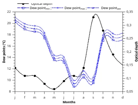
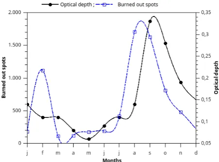
concomitantly with the optical depth as a function of the time along the year. All these values are obviously positively correlated as all their characteristics follow similar shapes. The second graphic shows the temperatures – minimum, maximum and average values – also with the optical depth. The third graphic shows the humidity factor, also minimum, maximum and average values as a function of the time along the year to be compared with the optical depth. Graphic number four shows the drew point while graphic number 5 represents the atmospheric pressure, minimum, maximum and average values of both variables. Graphics number 6 and number 7 show the wind direction and wind speed respectively. Graphic number 8 exhibits the solar radiation and graphic number 9 shows the clarity index. The last two graphics, numbers 10 and 11 shows the number of wildfires spots and the precipitation level, respectively, always compared, in the same figure, with the optical depth as a function of the time along the year.
Figure 1. Measurement of ozone (O3) – empty square – and carbon monoxide (CO) – empty circles – concentrations at left and optical depth – filled circle – at right as a function of the time along the year.
The average temperatures measured in the region are high in spring-summer, with September and October being the
hottest months (averages above 23 °C) and mild in autumn-winter, but rarely lower than 18 °C. June and July are the months with the lowest thermal averages, between 18 °C and 21 °C. The average rainfall reached by precipitation during the year present a distribution of 1330 mm.
Figure 2. Measurement of the temperature – minimum, average and maximum values –at left and optical depth – filled circle – at right as a function of the time along the year.
Figure 3. Measurement of the humidity – minimum, average and maximum values –at left and optical depth – filled circle – at right as a function of the time along the year.
The values of monthly and annual average recorded temperatures lead to the understanding that the spatial and seasonal variation of this climatic variable follows the characteristics of the region.
Figure 5. Measurement of the atmospheric pressure – minimum, average and maximum values –at left and optical depth – filled circle – at right as a function of the time along the year.
Figure 6. Measurement of the wind direction – empty square – at left and optical depth – filled circle – at right as a function of the time along the year.
Figure 7. Measurement of the wind speed – empty square – at left and optical depth – filled circle – at right as a function of the time along the year.
The highest thermal averages are observed from October to March, which correspond to the summer in the tropical climates in the Southern Hemisphere. October is the month having the highest averages, and it is the period characterized by the transition between the dry period and rainy.
Figure 8. Measurement of the global solar radiation – empty square – at left and optical depth – filled circle – at right as a function of the time along the year.
Figure 9. Measurement of the clarity index – empty square – at left and optical depth – filled circle – at right as a function of the time along the year.
Changes in atmospheric circulation patterns such as high evapotranspiration rates, low average wind speeds, incipient precipitation, and low air humidity favour the elevation of temperatures, indicating the beginning of summer. Another analysis that can be done from the average temperatures is that the thermal amplitudes observed between the months with higher and lower temperatures are very low, varying 4.0 ° C in average, between June (lower thermal averages) and October (warmer month).
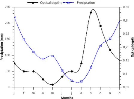
Figure 11. Measurement of the precipitation index – empty square – at left and optical depth – filled circle – at right as a function of the time along the year.
The rainy season goes from October to March/April and accounts for more than 85 % of annual rainfall, with the rains in December and January corresponding for more than 35% of the whole total. The dry season, which starts in April and lasts until the beginning of October, has a significant reduction in rainfall indices. The driest quarter of the year, from June to August, the rainfall represents, on average, less than 2 % of the annual total.
The dry season is characterized by long periods without rainfall or insignificant precipitations, well below the daily evapotranspiration (ETP), implying that the condition of environment dryness is not improved. These periods often exceed 100 days. For sake of analysis, periods of drought are defined as those which over 75 days remain without precipitation. During the period of study, there were many longer periods of drought above the minimum limit set. Considering the years for which longer periods of drought have been observed, the average number without rain is 105 days, the average number of days without significant precipitation (below than 2.5 mm) is 110 days. Practically half of the total number of years present long periods without rain exceeding 75 uninterrupted days. These periods coincide with the dry season of the year, being more common during June, July and August.
The variation of the aerosol concentrations in the atmosphere of Campo Grande - MS is strongly influenced by the biomass burning. The practice of biomass burning is related to the meteorological conditions observed during the second winter half and the first spring half. The long period without precipitation and relatively low relative humidity are meteorological factors that contribute to the seasonality of biomass burning (figure 1 on burning outbreaks).
The seasonality of the atmosphere contamination by aerosols for Campo Grande – MS has been verified. Critical periods occur typically between August and October, coinciding with the dry season. The values of the monthly averages of the optical thickness in the channel of 500 nm
(τ500nm) began rising on August (τ500nm ~ 0.1). Maximum
values usually occur in September (τ500nm ~ 0.5 to 1.0) and
decrease from October onwards with the onset of the rainy season. The decrease of the aerosol concentrations in the atmosphere due to the beginning of the rainy season varies from year to year.
The principal events associated with the most intense attenuation of aerosol radiation due to the decreasing number of heat sources have also been detected by the AVHRR/NOAA sensor and the movement analysis by the MODIS/TERRA sensor. The effect of aerosol reduction in the atmosphere due to the beginning of the rain season differs from year to year. The observed and analysed results indicate that some regions are can be considered the main contributors to the presence of aerosols in the atmosphere of Campo Grande - MS (Figure 9 - optical depth and clarity index).
DISCUSSION
To understand the temporal variation of aerosols in the studied area, the time series profile of the mean AOT values are presented in Figures 1 to 11. During the period of study, every maximum AOT value appeared during the spring, i.e. between October and December. The seasonal mean value of
τ500nm measures how the cyclical variations are different. In
2007 and 2010, seasonal mean values of τ500nm showed a
downward trend from spring to winter (July ~ September of the following year). Conversely, in 2008 and 2009, these measured values decreased from spring to autumn (April ~ June) and then increased slightly during the winter.
The annual cycle of seasonal averages shows a trend, which decreases first from May to October and then increases from November to April of the following year, and all maximums appear during the spring. Thus, in order to better understand these dissimilar cyclical variations, it is necessary to analyse the spatial and temporal variations of AOT. In all figures from
1 to 12, mean values of τ500nm reach the highest during the
spring, compared to the rest of the year.
Studies suggest that spring dust and local biomass firing activities in the north of the country may have caused an increase in the aerosol load in this area.10,11,28-31 In addition,
vast areas of agricultural lands are located in the vicinity of Campo Grande. After the spring harvest, local agricultural wastes (e.g. cane straw, corn, wheat straw and residual wood) are commonly burned to remove unwanted biomass and to control invasive pests.
Understandably, the increased deposition of coarse particles by precipitation elimination plays a dominant role. For the city of Campo Grande – MS, the population density may be considered medium. The agricultural productivity is pre-eminent and the winter is not very rigorous. The consumption of fossil fuels and biofuels are naturally large, contributing to SO2 emissions with a mean of 1.76 ppb,
varying from a minimum of zero and a maximum of 46.6 ppb during the year.29 The heavily emitted SO
2 can be largely
converted to sulfate aerosols in the atmosphere, making it the dominant component of aerosols in Campo Grande.
Sulfates are hygroscopic aerosols, while the size of their particle can grow with increasing humidity. The climate in Campo Grande, characterized by high humidity throughout the rainfall season, may be favourable for the growing single-spreading albedo (SSA) of sulfate aerosols. The SSA aerosol of sulfate doubles when RHU increases.35 Thus, in Campo
Grande, the meteorological conditions could contribute approximately equally with heavy emissions of SO2 to
increase the concentrations of particulate material, thus increasing the optical thickness. In addition, Campo Grande is located in a surrounding depression that prevents the horizontal dispersion of concentrated aerosols. Thus, the combined effects of heavy emissions, special weather conditions and negative relief forms can result in high AOT values.
Also, the fuel consumption of human activities in the city of Campo Grande, such as industrial production, heating, depletion of vehicles and daily life, releases waste gases with a large amount of AOT. In addition to the high RHU contributions, it can clearly increase the hygroscopicity of aerosol particles and reduce the dispersion of secondary pollutants, which can result in a larger increase in AOT.
Aerosols and meteorological factors
The temporal variations of AOT are affected mainly by the seasonal variations of the meteorological conditions and emissions of particulate material. Meteorological conditions affect AOTs in different ways, TEM and RHU affect the production of secondary particles,30.34 PREC affects
deposition34 and velocity affects dispersion.20 In addition,
changes in emissions of natural and anthropogenic particles are also closely related to weather conditions. Aerosols also have a considerable impact on atmospheric energy balance and weather conditions. Thus, to better understand the aerosol-meteorological interactions, the statistical properties of AOTs and meteorological factors shall be presented and discussed below.
AOT and meteorological variables
Using the Principal Component Analysis (ACP) extraction method with Varimax rotation and Kaiser normalization, and Cluster analysis obtained by the WARD method, two groups were obtained that explained 87.8 % of the total variance. This total is composed by the factor 1/group 1, which explains 51 % of the variance, and the factor 2/group 2, which explains 36.8 % of the variance.
Cluster analysis was performed, and the results show two separate groups, and within each group there are two
subgroups. They are, for group 1: subgroup 1.1 – ozone and carbon monoxide; subgroup 1.2 – outbreaks of burning. For group 2: subgroup 2.1 – average, maximum and minimum atmospheric pressure, maximum, minimum and average temperatures, and solar radiation; and subgroup 2.2 – mean dew point, maximum and minimum precipitation, maximum and minimum air humidity, clarity index, wind speed, and wind direction.
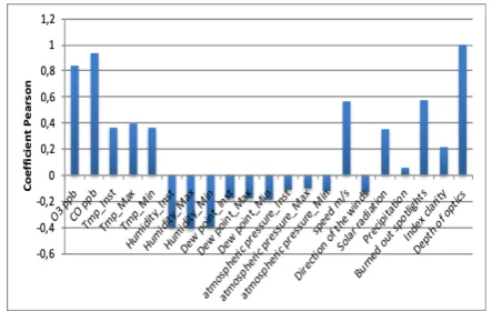
Figure 12. Pearson coefficients relating the studied variables and aerosols for Campo Grande – MS, Brazil.
No obvious relationship was found between AOT and meteorological variables. This may occur because the low-pressure climate is conducive to controlling the dilution and diffusion of air pollution, which plays a significant role in reducing pollution levels. In contrast, under high pressure conditions, higher concentrations of soil-level pollution have been observed in some scientific communications.36,37
The TEM is similar to the AOT pattern, which correlated positively. The next factor, RHU, shows a negative correlation. The PREC indicates a positive correlation. Thus, these results make it clear that high TEM and RHU may result in the increase of fine particles, and PREC can easily remove coarse particles, which are quite similar to the results of some recent published studies.32-33
During the summer and fall, TEM, RHU and PREC are all larger, resulting in relatively low AOT values. Conversely, during the spring and winter, TEM, RHU and PREC are all smaller, resulting in relatively higher AOT values. Continuing with EVP and SSD, the evaporation capacity is positively correlated with the duration of sunlight. In this study, the seasonal variations of EVP are also consistent with those of SSD and show approximately negative correlations with AOT. This indicates that reductions in evaporation and duration of sunlight seem to be related to rises in aerosol load, which is quite similar to earlier results.23,38
The seasonal mean of AOT is correlated to PRS, TEM, RHU and PREC, as fine particle aerosols are easier to accumulate when all four meteorological factors are at maximum.32,33,36 This is due to the fact that aerosols of coarse
particles can be easily removed by wet deposition and can result in the reduction of solar radiation that reaches the surface and reduces evaporation.23,34,38
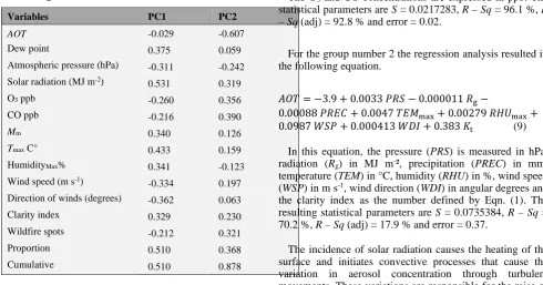
Table 1. Weight coefficients of the new PC variables.
Variables PC1 PC2
AOT -0.029 -0.607
Dew point 0.375 0.059
Atmospheric pressure (hPa) -0.311 -0.242
Solar radiation (MJ m-2)
0.531 0.319
O3 ppb -0.260 0.356
CO ppb -0.216 0.390
Mm 0.340 0.126
Tmax C° 0.433 0.159
HumidityMax% 0.341 -0.123
Wind speed (m s-1)
-0.334 0.197 Direction of winds (degrees) -0.362 0.063
Clarity index 0.329 0.230
Wildfire spots -0.212 0.321
Proportion 0.510 0.368
Cumulative 0.510 0.878
PCA Results
New variables with unique physical interpretations were found from PCA data that can be inferred from the weighting coefficients used to create each variable (Table 1). The first PC variable (PC1) accounts for 51 % of the total variance and is derived mainly from the predominant meteorological factors. Positive values of PC1 were obtained for vapour pressure, precipitation, temperature, and humidity. In addition, PC1 also receives negative weights of atmospheric pressure and wind speed. Thus, it can be inferred that the positive values of PC1 are clearly indicative of atmospheric conditions in which the low pressure, the air dryness and the longer duration of the insolation are more likely to occur. Such atmospheric conditions are conducive to controlling the dilution and diffusion of fine particles, which results in relatively low AOT – negative values.
The PC2, which represents 36.8 % of the total variance, reveals a more interesting interaction between the pollutant and aerosol variables. In particular, the positive sign of the ozone coefficient is consistent with carbon monoxide because the weighting coefficients obtained for them are almost equal. Thus, the positive values of PC2 correspond to high values of ozone and CO, which play an important role in increasing AOT.
If the data are correlated, the model should be adjusted taking into account these auto correlations. This correction is done by inserting the residue into the model. All considerations on temporal trends should be observed when conducting a study, for example, on the impact of a particular variable. Other factors that are generally considered in these studies are the effects of temperature, precipitation and humidity. After considering the mentioned factors, the values of the coefficients, β, are determined. For the group 1, the values of regression analysis yielded the following results.
𝐴𝐴𝑂𝑂𝐴𝐴= 0.0643−0.00133 O3+ 0.000446 CO−
0.000006 𝑤𝑤𝑤𝑤𝑤𝑤𝑤𝑤𝑤𝑤𝑤𝑤𝑤𝑤𝑤𝑤𝑤𝑤 (8)
The O3 and CO-concentrations are expressed in ppb. The
statistical parameters are S = 0.0217283, R – Sq = 96.1 %, R – Sq (adj) = 92.8 % and error = 0.02.
For the group number 2 the regression analysis resulted in the following equation.
𝐴𝐴𝑂𝑂𝐴𝐴=−3.9 + 0.0033 𝑃𝑃𝑅𝑅𝑀𝑀 −0.000011 𝑅𝑅g−
0.00088 𝑃𝑃𝑅𝑅𝑀𝑀𝑃𝑃+ 0.0047 𝐴𝐴𝑀𝑀𝑀𝑀max+ 0.00279 𝑅𝑅𝑅𝑅𝑅𝑅max+
0.0987 𝑊𝑊𝑀𝑀𝑃𝑃+ 0.000413 𝑊𝑊𝑊𝑊𝑊𝑊+ 0.383 𝐾𝐾t (9)
In this equation, the pressure (PRS) is measured in hPa, radiation (Rg) in MJ m-², precipitation (PREC) in mm,
temperature (TEM) in °C, humidity (RHU) in %, wind speed (WSP) in m s-1, wind direction (WDI) in angular degrees and
the clarity index as the number defined by Eqn. (1). The resulting statistical parameters are S = 0.0735384, R – Sq = 70.2 %, R – Sq (adj) = 17.9 % and error = 0.37.
The incidence of solar radiation causes the heating of the surface and initiates convective processes that cause the variation in aerosol concentration through turbulent movements. These variations are responsible for the raise or reduction in aerosol concentration within a certain volume from both horizontal and vertical motion.
Environmental degradation is one of the main problems of modern society. Technological development, population growth and its concentration in the urban environment, industrialization and the use of new methods and techniques in agriculture are some of the contributing factors for the introduction of different chemical, synthetic and even natural substances into the environment, which generate adverse effects on the environment and living things.
CONCLUSION
The local averages of seasonality, considering the crests and depressions of the curve, indicating the increased concentration of aerosols observed during the analysis can be attributed: (i) to the dust aerosols produced locally from desert zones and catalyzed by intense solar heating also as transported aerosols; (ii) to the increase in anthropogenic activities, as the land preparation and biomass burning that release a significant amount of dust and smoke particles into the atmosphere; (iii) to the smoke particles transported from neighbouring countries and neighbouring states – the southern part of Campo Grande is called the arc of fire, region where there is a higher incidence of wildfires; and (iv) to the atmospheric inversion condition prevalent in the region, which does not withstand upward movement of air resulting in high aerosol loading at the lower levels of the atmosphere. The low AOT observed during the local moist months can be attributed to the reduction of anthropogenic activities and the increase of wet deposition processes.
95 % confidence level) between AOT and precipitation (Figure 12). Generally, precipitation can affect aerosol loading, especially dust particles in different ways: (i) it washes aerosols by reducing their concentration in the atmosphere, a process known as elimination; (ii) increases soil moisture by suppressing induced dust emissions as winding the ground. In addition, it increases the growth of the vegetation, which could also prevent the emission of dust. However, during periods of drought, the residue varies freely due to the aerosol emissions from burnings and biomass events.
In this study, the aerosol and meteorological data were analysed to assess the relationships between aerosols and meteorological conditions. The aerosol distribution properties have first been examined in the research area and found that the temporal variations of the AOT show different characteristics and are mainly affected by variations in meteorological conditions and particulate emissions. A main result of this work is that the seasonal annual cycle of AOT shows a decreasing trend followed by a rise, and all highs appear in the spring.
The variability of AOT in the 500 nm channel verified in the atmosphere of Campo Grande – MS presents a strong monthly seasonality related to the predominant meteorological conditions and to the numerous fires of burnings verified in regions that are source of aerosols. In the months with the greatest influence of the wildfires, monthly
averages of τ500nm from 0.6 to 1.0 were observed, while in the
months with cleaner atmosphere values of τ500nm were
observed around 0.1. The mathematical correlation between the climatic indicators indicated that the main source in order of significance formed two groups, with two subgroups each.
The analysis of the temporal variability of AOT showed that Campo Grande has a characteristic annual cycle with increase of AOT in the periods of August to October, with maximums recorded in the month of September, coinciding with the period of increase of burnings in the southern Amazon and in the areas of the Brazil Central-West “cerrado”, while in the other months of the year AOT has low values, around 0.1.
It was observed that the years presenting the highest AOT load in the region were those in which there were a greater number of outbreaks of burning in the Brazilian territory. The atmospheric circulation and frontal systems that operate in South America during the dry season period interfere in the amount of foci and, consequently, in the AOT values for several regions, including Campo Grande, which is one of the places, affected by the air masses that aerosol from the northern region.
FUNDING
This research received no external funding. Flavio Aristone is thankful to CNPq for financial support.
ACKNOWLEDGMENTS
The authors thank their Universities for their support.
DATABASE STATEMENT/DATA
AVAILABILITY
The climate database is public domain and available at: INMET: http://www.inmet.gov.br/portal/index.php?r= esta-coes/estacoesAutomaticas;https://giovanni.gsfc.nasa.gov/gio vanni; http://climan alise.cptec.inpe.br/~rclimanl/boletim/
REFERENCES
1Chen, S., Zhao, C., Qian, Y., Leung, L. R., Huang, J.-P., Huang, Z.-W., Bi, J.-R., Zhang, Z.-W., Shi, J.-S., Yang, L., Li, Deshuai, Li, J. X., Regional modeling of dust mass balance and radiative forcing over East Asia using WRF-Chem,Aeolian Res., 2014, 15, 15–30. https://doi.org/10.1016/j.aeolia.2014.02.001
2Gui, Ke; Che, Huizheng; Chen, Quanliang; Zeng, Zhaoliang; Zheng, Yu; Long, Qichao; Sun, Tianze; Liu, Xinyu; Wang, Yaqiang; Liao, Tingting; Yu, Jie; Wang, Hong; Zhang, Xiaoye. Water vapor variation and the effect of aerosols in China, Atm. Environ., 2017, 165, 322–335. DOI: 10.1016/j.atmosenv.2017.07.005
3Brock, C. A., Cozic, J., Bahreini, R., Froyd, K. D., Middlebrook, A. M., McComiskey, A., Brioude, J., Cooper, O. R., Stohl, A., Aikin, K. C., de Gouw, J. A., Fahey, D. W., Ferrare, R. A., Gao, R.-S., Gore, W., Holloway, J. S., Hübler, G., Jefferson, A., Lack, D. A., Lance, S., Moore, R. H., Murphy, D. M., Nenes, A., Novelli, P. C., Nowak, J. B., Ogren, J. A., Peischl, J., Pierce, R. B., Pilewskie, P., Quinn, P. K., Ryerson, T. B., Schmidt, K. S., Schwarz, J. P., Sodemann, H., Spackman, J. R., Stark, H., Thomson, D. S., Thornberry, T., Veres, P., Watts, L. A., Warneke, C., and Wollny, A. G.: Characteristics, sources, and transport of aerosols measured in spring 2008 during the aerosol, radiation, and cloud processes affecting Arctic Climate (ARCPAC) Project, Atm. Chem. Phys., 2011, 11, 2423–2453, https://doi.org/10.5194/acp-11-2423-2011.
4Qian, Y. U. N., Leung, L. R., Ghan, S. J., Giorgi, F., Regional climate effects of aerosols over China: Modeling and observation, Tellus B Chem. Phys. Meteorol., 2011, 55(4), 914–934. doi.org/10.3402/tellusb.v55i4.16379
5 Levy H, Horowitz L, Schwarzkopf M, Ming Y, Golaz J, Naik V, Ramaswamy V. The roles of aerosol direct and indirect effects in past and future climate change, J. Geophys. Res. Atmos.,
2013, 118(10), 4521–4532. doi.org/10.1002/jgrd.50192
6Gao, Y., Liu, X., Zhao, C., Zhang, M., Emission controls versus meteorological conditions in determining aerosol concentrations in Beijing during the 2008 Olympic Games, Atm. Chem. Phys., 2011, 11, 16655–16691. DOI: 10.5194/acpd-11-16655-2011
7Zhang, Z., J. Wang, L. Chen, X. Chen, G. Sun, N. Zhong, H. Kan, and W. Lu. Impact of haze and air pollution-related hazards on hospital admissions in Guangzhou, China. Environ. Sci. Pollut. Res., 2014, 21, 4236–4244. doi: 10.1007/s11356-013-2374-6
8Lu F, Xu D, Cheng Y, Dong S, Guo C, Jiang X, Zheng X, Systematic review and meta-analysis of the adverse health effects of ambient PM2.5 and PM10 pollution in the Chinese population, Environ. Res. 2015, 136, 196–204. doi: 10.1016/j.envres.2014.06.029.
9Mukherjee, A., Agrawal, M., World air particulate matter: sources, distribution and health effects, Environ. Chem. Lett., 2017, 15(2), 283–309).
10Souza, A. Santos, D. A. S., Lariane, P. G. C., Poluição Atmosférica Urbana A Partir De Dados De Aerossóis Modis: Efeito Dos Parâmetros Meteorológicos, Boletim Goiano de Geografia,
2017, 37, 466. doi.org/10.5216/bgg.v37i3.50766
11Souza, A., Ihaddadene, R., Ihaddadene, N., Oguntunde, P. E., Clarity Index Analysis and Modeling Using Probability Distribution Functions in Campo Grande-MS, Brazil, J. Sol. Energy Eng., 2019, 141(6), 061001.
12Steiner, W. A., The influence of air pollution on moss-dwelling animals, I, Methodology and composition of flora and fauna, Rev. Suisse Zool., 1994, 101(2), 533–556.
https://doi.org/10.5962/bhl.part.79917
13Shang, H., Chen, L., Tao, J., Lin, S., Jia, S., Synergetic use of MODIS cloud parameters for distinguishing high aerosol loadings from clouds over the North China Plain. IEEE. J. Sel. Top. Appl. Earth Obs. Remote Sens., 2014, 7(12), 4879– 4886. DOI: 10.1109/JSTARS.2014.2332427
14Zhang Z., Wu W., Wei J., Song Y., Yan X., Zhu L., Wang Q., Aerosol optical depth retrieval from visibility in China during 1973–2014, Atm. Environ., 2017, 171, 38–48. DOI: 10.1016/j.atmosenv.2017.09.004
15Che, H., Zhang, X.-Y., Xia, X., Goloub, P., Holben, B., Zhao, H., Wang, Y., Zhang, X.-C., Wang, H., Blarel, L., Damiri, B., Zhang, R., Deng, X., Ma, Y., Wang, T., Geng, F., Qi, B., Zhu, J., Yu, J., Chen, Q., and Shi, G.. Ground-based aerosol climatology of China: aerosol optical depths from the China Aerosol Remote Sensing Network (CARSNET) 2002–2013, Atm. Chem. Phys., 2015, 15(13), 7619–7652.
https://doi.org/10.5194/acp-15-7619-2015
16Filonchyk, M., Yan, H., Zhang, Z., Analysis of spatial and temporal variability of aerosol optical depth over China using MODIS combined Dark Target and Deep Blue product, Theor. Appl.Climatol, 2018, 1–18,
https://doi.org/10.1007/s00704-018-2737-5.
17Sarkar, T., Mishra, M., Soil Erosion Susceptibility Mapping with the Application of Logistic Regression and Artificial Neural, Network. J. Geovis. Spat. Anal., 2018, 2(1), 8.
https://doi.org/10.1007/s41651-018-0015-9.
18Dawson, J. P., Adams, P. J., Pandis, S. N., Sensitivity of PM2.5 to climate in the Eastern US: A modeling case study, Atmos. Chem. Phys., 2007, 7(16), 4295–4309, doi:10.5194/acp-7-4295-2007.
19Dawson, J. P., Racherla, P. N., Lynn, B. H., Adams, P. J., Pandis, S. N., Impacts of climate change on regional and urban air quality in theeastern United States: Role of meteorology, J. Geophys. Res., 2009, 114, D05308, doi:10.1029/2008JD009849.
20Deng, X., Shi, C., Wu, B., Chen, Z., Nie, S., He, D., Zhang, H., Analysis of aerosol characteristics and their relationships with meteorological parameters over Anhui province in China, Atm. Res., 2012, 109–110(0), 52–63,
doi:10.1016/j.atmosres.2012.02.011.
21Jiménez-Guerrero, P., Montávez, J. P., Gómez-Navarro, J. J., Jerez, S., Lorente-Plazas, R., Impacts of climate change on ground levelgas-phase pollutants and aerosols in the Iberian Peninsula for the late XXI century, Atm. Environ., 2012, 55(0), 483–495, doi:10.1016/j.atmosenv.2012.02.048.
22Yang, X., Ferrat, M., Li, Z. Q., New evidence of orographic precipitation suppression by aerosols in central China, Meteorol. Atm.. Phys., 2013, 119(1–2), 17–29, doi:10.1007/s00703-012-0221-9
23Wang, Y. W., Yang, Y. H., China’s dimming and brightening: Evidence, causes and hydrological implications, Ann. Geophys., 2014, 32(1), 41–55, doi:10.5194/angeo-32-41-2014.
24Latorre, M., Cardoso, M., Análise De Séries Temporais Em Epidemiologia: Uma Introdução Sobre Aspectos Metodológicos, Rev. Bras. Epidemiol., 2014, 4(3), 145-152.
25Montgomery, D. C., Peak, E. A., Introduction to linear regression analysis.2nd Ed., Wiley, New York, 1992, 68-79.
26Abdi, H., Williams, L. J., Principal component analysis, WIREs Comp. Stat., 2010, 2(4), 433–459. doi:10.1002/wics.101.
27Jones, T. A., Christopher, S. A., Statistical properties of aerosol-cloud-precipitation interactions in South America, Atm. Chem. Phys., 2010, 10(5), 2287–2305, doi:10.5194/acp-10-2287-2 010.
28Souza, A., Santos, D. A. S., Análise das componentes principais no processo de monitoramento ambiental, Nativa, 2018, 6, 639. http://dx.doi.org/10.31413/nativa.v6i6.6453
29Souza,A., Santos,D.A.S., Aristone,F., Kovač-Andrić,F.,
Marković,B., Matasović,B., Pavao,H.G., Pires,J.C.M., Ikefuti,
P.V.,Impacto De Fatores Meteorológicos Sobre As Concentrações De Ozônio Modelados Por Análise De Séries Temporais E Métodos Estatísticos Multivariados, Holos
(Natal. Online), 2017, 5, 2.
DOI: https://doi.org/10.15628/holos.2017.5033
30Souza, A., Ikefuti, P. V, Garcia, A. P., Santos, D. A. S, Oliveira, S., Análise da relação entre O3, NO e NO2 usando técnicas de regressão linear múltipla, Geographia (UFF), 2018, 20, 124.DOI: 10.22409/geographia.v20i43.1065
31Souza, A., Jan, B., Nawaz, F., Zai, M.A.K.Y., Oliveira, S.S., Pavao, H.G.,Fernandes, W.A., Ihaddadene, R., Ihaddadene, N., Oguntunde, P.E., Santos, D.A.S.., Temporal variations of SO2 in an urban environment, Discovery, 2019, 55(283), 328-339.
32Lee, K. H., Kim, Y. J., von Hoyningen-Huene, W., Burrow, J. P., Spatio-temporal variability of satellite-derived aerosol optical thickness over Northeast Asia in 2004, Atm. Environ., 2007, 41(19), 3959–3973, doi:10.1016/j.atmosenv.2007.01.048
33Che, H. Z., Zhang, X. Y., Alfraro, S., Chatenet, B., Gomes, L., Zhao, J. Q., Aerosol optical properties and its radiative forcing over Yulin, China in 2001 and 2002, Adv. Atm. Sci., 2009, 26(3), 564–576, doi:10.1007/s00376-009-0564-4
34Tao, J., Zhang, L., Engling, G., Zhang, R., Yang, Y., Cao, J., Zhu, C., Wang, Q., Luo, L., Chemical composition of PM2.5 in an urban environment in Chengdu, China: Importance of springtime dust storms and biomass burning, Atm. Res., 2013, 122(0), 270–283, doi:10.1016/j.atmosres.2 012.11.004.
35Thornhill, G. D., Ryder, C. L., Highwood, E. J., Shaffrey, L. C., Johnson, B. T., The effect of South American biomass burning aerosol emissions on the regional climate, Atm. Chem. Phys.,
2018, 18, 5321–5342. https://doi.org/10.5194/acp-18-5321.
36Chen, Z. H., Cheng, S. Y., Li, J. B., Guo, X. R., Wang, W. H., Chen, D. S., Relationship between atmospheric pollution processes and synoptic pressure patterns in northern China, Atm. Environ., 2008, 42(24), 6078–6087. doi:10.1016/j.atmosenv.2008.03.043.
37Im, U., Tayanc, M., Yenigun, O., Analysis of major photochemical pollutants with meteorological factors for high ozone days in Istanbul, Turkey, Water Air Soil Pollut., 2006, 175(1–4), 335– 359. doi:10.1007/s11270-006-9142-x.
38Sanchez-Lorenzo, A., Calbó, J., Wild, M., Azorin-Molina, C., and Sanchez-Romero, A.: New insights into the history of the Campbell-Stokes sunshine recorder, Weather, 2013, 68, 327– 331, doi:10.1002/wea.2156.