A STABLE METHOD FOR LINEAR EQUATION
IN BANACH SPACES WITH SMOOTH NORMS
1Andrey A. Dryazhenkov† and Mikhail M. Potapov††
Lomonosov Moscow State University, Leninskie Gory, Moscow, Russia, 119991 †andrja@yandex.ru, ††mmpotapovrus@gmail.com
Abstract: A stable method for numerical solution of a linear operator equation in reflexive Banach spaces is proposed. The operator and the right-hand side of the equation are assumed to be known approximately. The corresponding error levels may remain unknown. Approximate operators and their conjugate ones must possess the property of strong pointwise convergence. The exact normal solution is assumed to be sourcewise representable and some upper estimate for the norm of its source element must be known. The norm in the Banach space of solutions is supposed to satisfy the following smoothness-type condition: some function of the norm must be differentiable. Under these conditions a stability of the method with respect to nonuniform perturbations in operator is shown and the strong convergence to the normal solution is proved. A boundary control problem for the one-dimensional wave equation is considered as an example of possible application. The results of the model numerical experiments are presented.
Keywords:Linear operator equation, Banach space, Numerical solution, Stable method, Sourcewise repre-sentability, Wave equation.
Introduction
The problem of finding solution to a linear operator equation arises in many fields of applied mathematics when solving integral equations, some boundary value problems, systems of linear equations and other linear inverse problems. The known complication that can arise thereby is the ill-posedness of such inverse problems. This means that small changes in initial data (coefficients of the system of linear equations, the right-hand sides of equations, boundary data, coefficients of differential operator, etc.) can cause loss of existence or uniqueness of the perturbed problem solution or lead to not small changes in this solution. To deal with the issues of such types many regularization methods were proposed: Tikhonov regularization method [23, 24], residual method [17], method of quasi-solutions [12], residual principle [16], iterative regularization methods [2] and many others [3,10,21, 22,25]. Most of them require knowledge of error levels in initial data approximation or knowledge of some compact set containing a sought solution. In many applications these assumptions are rather hard to be ensured. Instead of these traditional assumptions our method requires a sought solution to be sourcewise representable and, moreover, some majorant for the source norm to be known. It allows anyone who wants to apply the method to focus on researching corresponding properties of the exact problem.
In this paper we consider a linear operator equation
Au=f (1)
in reflexive Banach spacesH andF,whereA ∈ L(H →F) is a linear bounded operator andf ∈F is a given element. It is required to find normal solutionu∗, i. e. a solutionu∗ to (1) with a minimal
1
norm in the space H:
u∗ = arg min
u∈UkukH, U ={u∈H| Au=f}. (2)
In the sequel the norm of the spaceH will be supposed to be strictly convex, so the solutionu∗ to the problem (2) is unique, and it exists if equation (1) has a solution [8, Proposition 1.2, p. 35].
Suppose that instead of exact dataAandf some of their approximations An∈ L(H→F) and
fn ∈ F, n= 1,2. . . , are known. The asymptotic properties of the method will be studied under
the condition that the approximate data converge to the exact ones in the following sense:
kAnu− AukF →0, ∀u∈H, kAn∗v− A∗vkH∗ →0, ∀v∈F∗, kfn−fkF →0 as n→ ∞.
(3)
Here and belowA∗:F∗ →H∗andA∗n:F∗→H∗ are operators adjoint toAandAn.Note that the
first two limit relations in (3) are weaker than conditions of uniform convergence usually required in the traditional regularizing procedures [3, 10,16], [22] – [25]. Also we do not require in (3) the knowledge of any error levels.
A stable method of solving the problem (2) under perturbations of type (3) in Hilbert spaces H and F was proposed in [19]. Briefly recall this method for the convenience of comparison. In [19] the following basic assumptions were accepted:
H1. Spaces H and F are Hilbert and identified with their adjoint spaces in the Riesz sense: H ≃ H∗, F ≃F∗.
H2. Equation (1) has a solution.
H3. The solution u∗ to (2) is sourcewise representable: u∗ ∈ R(A∗), where R(A∗) denotes range of operator A∗ :F →H. It means that there exists a source elementv∗ ∈F such thatu∗ =A∗v∗.
H4. Some majorant r∗ of the source norm is known: kv∗kF ≤r∗.
It is well-known that the solution u∗ to (2) belongs to the closure of R(A∗) [10, Proposition 2.3, p. 33], so the assumption H3 is rather natural and holds true for any operatorAwith closed range. The method from [19] is then formulated as follows: find a solution vn ∈ F to the following
quadratic optimization problem
In(vn)≤ inf
v∈V In(v) +εn, εn≥0,
V ={v∈F| kvkF ≤r∗}, In(v) =
1 2kA
∗
nvk2H − hv, fniF,
(4)
and set element un = A∗nvn as a final approximation for the sought solution to (2). Here h·,·iF
denotes the inner product in spaceF.
Theorem 1 [19]. Let assumptions (3),H1–H4 be fulfilled, let un be an output of the described
method and εn→0 as n→ ∞. Then the convergence kun−u∗kH →0 holds true.
The method proposed below is an extension of the described method from [19] to Banach spaces with smoothness-type property of the norm in space H.
1. Basic Assumptions and Auxiliary Statements
The method presented in the next section for Banach spaces requires the following assumptions:
B1. H and F are reflexive Banach spaces.
B2. The norms inH and H∗ are strictly convex.
B3. For the norm in H∗ the Radon–Riesz property holds true: if sequence {gn} ⊂ H∗ converges
weakly tog0 ∈H∗: gn→w g0, and the corresponding sequence of norms also converges: kgnkH∗ → kg0kH∗, then the sequence{gn}converges strongly: kgn−g0kH∗ →0.
B4. Let φ∈C[0,+∞[ be a continuous strictly increasing function, φ(0) = 0, φ(+∞) = +∞ and let φ−1 be inverse ofφ. Let two functionalsP :H→Rand K :H∗ →R are defined as
P(u) =p(kukH), p(x) =
Z x
0
φ(ξ)dξ,
K(g) =k(kgkH∗), k(x) =
Z x
0
φ−1(ξ)dξ.
(1.1)
These functional are assumed to be Fr´echet differentiable: P ∈C1(H),K ∈C1(H∗).
B5. Equation (1) has a solution.
B6. The solutionu∗ to (2) is sourcewise representable in the following sense: there exists an element v∗ ∈F∗ such that u∗ =JHA∗v∗, where mapping JH :H∗→H is defined as
JHg=K′(g), ∀g∈H∗. (1.2)
B7. Some majorant r∗ of the source norm is known: kv∗kF∗ ≤r∗.
Remark 1. Using reflexivity of H and Asplund’s duality mapping representation theorem [5, Theorem 4.4, p. 26], it is not hard to see that JH defined in (1.2) is in fact duality mapping
with weight (or gauge) functionφ−1(x).
Let us explain the meaning of the assumption B6. As in the case of Hilbert spaces H and F, this assumption is fulfilled for operators A with closed range. The corresponding proof will be presented now.
Theorem 2. Let assumptions B1, B2, B4, B5 be fulfilled and Au∗ =f. Then u∗ is solution to (2) if and only if
P′(u∗)∈R(A∗), (1.3)
where R(A∗) is closure ofR(A∗).
P r o o f. Letu∗ be a solution to (2). Let us prove that (1.3) takes place. Consider the following minimization problem:
P(u)→min, Au=f. (1.4)
Since functionp(x) is strictly increasing andP(u) =p(kukH), this problem is equivalent to (2), and
the elementu∗ is the unique solution to (1.4). Also consider linear auxiliary minimization problem:
Here and below, the expression hf, ui is understood as the value of linear continuous functional f ∈ H∗ on the element u ∈ H. Notice that optimal value of minimizing functional in (1.5) is nonnegative. Indeed, if there exists an element ub∈H such that hP′(u
∗),ubi<0 and Aub= 0, then we can consider elements uα =u∗+αu,b α≥0. Using definition of Fr´echet derivative we get
P(uα) =P(u∗) +αhP′(u∗),ubi+o(α),
where o(α)/α → 0 as α → 0. It means that for all sufficiently small α > 0 P(uα) < P(u∗) and Auα =Au∗+αAub=Au∗ =f, so u∗ is not the solution to (1.4). This contradiction shows that hP′(u
∗), ui ≥ 0 for all u ∈ H such that Au = 0, i. e. for all u ∈ N(A), where N(A) denotes the kernel ofA. Since the kernel N(A) is a linear subspace of H,it means that hP′(u∗), ui= 0 for all u∈N(A). In other words, we have
P′(u∗)∈(N(A))⊥, (N(A))⊥={g∈H∗| hg, ui= 0, ∀u∈N(A)}, (1.6)
and equality (N(A))⊥=R(A∗) (see [13, Theorem 1∗, p. 357], using reflexivity ofH) allows us to pass from (1.6) to (1.3).
On the other hand, let u∗ be a solution to (1) and let inclusion (1.3) be fulfilled. We want to prove that u∗ =u, whereb bu is a solution of (2). Let us suppose that u∗ 6=u. Notice that underb assumptions B2, B4 operator P′(u) is strictly monotonic and that is why the following inequality holds true:
hP′(u∗)−P′(bu), u∗−ubi>0. (1.7) It was proved above that ubsatisfies the condition (1.3), therefore P′(u∗)−P′(u)b ∈R(A∗). With inequality (1.7) it implies that there exists an element bv ∈ F∗ such that hA∗v, ub ∗−ubi > 0, but hA∗v, ub
∗−ubi = hbv,Au∗ − Abui = hbv, f−fi = 0. This contradiction means that our assumption u∗ 6=ubis not true, so u∗ is indeed a solution to (2).
Lemma 1. Let assumptions B1, B2, B4 be fulfilled. Then K′(P′(u)) = u, ∀u ∈ H and P′(K′(g)) =g, ∀g∈H∗.
P r o o f. Let us extend functions p(x) and k(x) defined in (1.1) to the region x ≤ 0 in the even way: k(x) = k(−x), p(x) = p(−x). Then these extensions will be convex dual. Indeed, for all x ∈R concave function xy−k(y) of variable y attains its maximum when x−k′(y) = 0, i. e. φ−1(y) =x. It means that
sup
y∈R
(xy−k(y)) =xφ(x)−k(φ(x)) =xφ(x)−
Z φ(x)
0
φ−1(ξ)dξ. (1.8)
Note that the following equality takes place for any strictly increasing smooth functionψ∈C1(R):
xψ(x)−
Z ψ(x)
0
ψ−1(ξ)dξ=xψ(x)−
Z x
0
χψ′(χ)dχ=
Z x
0
ψ(χ)dχ. (1.9)
Passing in (1.9) to the limit asψ→φ,ψ−1→φ−1 uniformly on any segment [a, b], we obtain from
(1.8) that
k∗(x) = sup
y∈R
(xy−k(y)) =
Z x
0
φ(χ)dχ=p(x), ∀x∈R,
K(g) =k(kgkH∗) (see [8, Proposition 4.2, p.19] ). Finally, we pass to the lemma statement using the relation between subgradients of dual functions [8, Corollary 5.2, p. 22].
Applying lemma1to (1.3) and using notation (1.2) we get the main result concerning assump-tion B6.
Corollary 1. Let assumptions B1, B2, B4, B5 be fulfilled and let u∗ be a solution to (1): Au∗ =f. Then u∗ is solution to (2) if and only if
u∗ ∈ JHR(A∗). (1.10)
It means that assumption B6 is fulfilled for all operators A with closed range. For other operators this assumption contains additional requirement to the normal solution u∗, but it is rather close to the necessary condition (1.10).
2. Description of the Method
The algorithm proposed below in Banach spaces to find the normal solution (2) to the equa-tion (1) in case of approximate data An, fn, n = 1,2, . . . , is similar to its Hilbert version (4)
from [19].
1. For the fixed sequence numbern find an element vn∈V that satisfies the conditions
In(vn)≤ inf
v∈V In(v) +εn,
V ={v∈F∗| kvkF∗ ≤r∗}, In(v) =K A∗nv
− hv, fni,
(2.1)
where r∗ is taken from assumption B7 and εn ≥ 0 is a parameter that allows to solve the
optimization problemIn(v)→inf, v∈V approximately.
2. Set un=JHA∗nvn as an approximate solution to (2).
Remark 2. Note that for Hilbert spaces H and F we can take φ(x) = φ−1(x) = x. Then K(u) =P(u) =kuk2
H/2 andJHu =K′(u) =u. In this case method (2.1) fully coincides with the
method from [19].
Remark 3. As in [19] instead ofV we can use in (2.1) sets
Vn={v∈Fn∗| kvkF∗ ≤r∗},
where Fn∗ is a closed subspace of F∗ such that An∗Fn∗ = R(A∗n). In this case the proof of the method convergence does not change. For finite-dimensional approximate operators An and A∗n
which are usually used in practical computations, it makes possible to choose finite-dimensional subspaces Fn∗ for variations of sources v. In this case, problem In(v) → inf, v ∈ Vn turns into
a finite-dimensional problem of minimization a smooth convex function In(v) on a ball Vn.Note
3. Proof of Convergence
Let us examine the behavior of the approximate solutions un when perturbed data An, fn
asymptotically approach their exact values A, f in the sense of (3). To do this we need the following equivalent reformulation of the problem (2).
Lemma 2. Let assumptions B1, B2, B4–B6be fulfilled. Then an elementu∗ ∈H is the solution to (2) if and only if it can be represented as u∗ =JHA∗vb, where bv is a solution to the following
optimization problem:
K(A∗v)− hv, fi →min, v ∈F∗. (3.1)
P r o o f. The problem (3.1) is a smooth and convex one without constraints, so it is equivalent to finding an elementv∈F∗ on which the derivative of the functional vanishes [8, Proposition 2.1, p. 36]:
AK′(A∗v)−f = 0.
Taking into account (1.2), this equation is equivalent to a system of two equations for the unknowns (u, v)∈H×F∗:
Au=f, u=JHA∗v. (3.2)
Let u∗ be a solution to (2). Then it follows from assumption B6 that u∗ satisfies (3.2). On the other hand, ifu∗ satisfies (3.2) then using corollary1 we get that u∗ is the solution to (2).
Now we are ready to prove convergence of the method.
Theorem 3. Let assumptions B1–B7 and conditions (3) be fulfilled. Let un be a final output
of the method described above and εn→0 as n→ ∞.Then kun−u∗kH →0 as n→ ∞.
P r o o f. Space F∗ is reflexive, and set V defined in (2.1) is convex, bounded and closed, therefore family vn ∈ V has in F∗ a weak limit point v0 ∈ V [7, V. 4.7, p. 425]: vnm
w
→ v0 as
m→ ∞. In order to simplify notation, we will omit symbolm from the subsequencenm and write
vn→w v0,n→ ∞. Then due to the strong pointwise convergence of An to Awe have
A∗nvn→ Aw ∗v0. (3.3)
FunctionalK(g) is convex and continuous, hence it is weakly lower semicontinuous [9, Proposition 5, p. 74]. Denote I(v) =K(A∗v)− hv, fi and notice that the following inequalities are valid:
I(v0)≤limIn(vn)≤limIn(vn)≤lim In(v0) +εn=I(v0). (3.4)
The first inequality in (3.4) is due to weak lower semicontinuity of K(g) and strong convergence kfn−fkF → 0. The third inequality follows from (2.1) and the inclusion v0 ∈V. The equality is
due to (3). From (3.4) it follows that there exists limIn(vn) =I(v0),i. e.
K A∗nvn− hvn, fni →K(A∗v0)− hv0, fi.
Since hvn, fni → hv0, fi we also have
K(A∗nvn)→K(A∗v0), kA∗nvnkH∗ → kA∗v0kH∗, (3.5)
where the last convergence takes place because the functionk(x) is strictly increasing. Using (3.3), (3.5) and Radon–Riesz property of norm from assumption B3, we get strong convergence
Since source element v∗ from assumption B6 belongs to V, it follows from (2.1) that In(vn) ≤
In(v∗) + εn. Passing to a limit and using (3.6) and convergence hvn, fni → hv0, fi, we get
I(v0)≤I(v∗). Lemma2 states that v∗ is a solution to global optimization problem (3.1). That is why
I(v0) =I(v∗)≤I(v), ∀v∈F∗.
This means that v0 is also a solution to the problem (3.1), so using lemma 2 once more, but in
opposite direction, we obtain that the only solution u∗ to the problem (2) can be represented by the sourcev0:
u∗=JHA∗v0.
Assumption B4 implies strong continuity of JH, which with (3.6) leads to the limit relation
kun−u∗kH =kJHA∗nvn− JHA∗v0kH →0. (3.7)
Notice that our proof holds true for all weak limit pointsv0 ∈V, and that is why convergence (3.7)
is valid for arbitrary family of approximate dataAn, fn possessing asymptotic properties (3).
4. Application to the Boundary Control Problem
In order to illustrate the application ability of the method, consider the following model bound-ary control problem for one-dimensional wave equation:
ytt(t, x) =yxx(t, x), (t, x)∈(0, T)×(0, l),
y|x=0=u(t), y|x=l= 0, t∈(0, T),
y|t=0 = 0, yt|t=0= 0, x∈(0, l).
(4.1)
The goal of control actions u(t) is to drive the system to a given final state f(x) = (f0(x), f1(x)) at a given time T ≥2l:
y|t=T =f0(x), yt|t=T =f1(x), x∈(0, l). (4.2)
The spaces H and F of controls u(t) and target statesf(x) are the following ones:
H=Lp(0, T), F =Lp(0, l)×Wp−1(0, l), 1< p <∞. (4.3)
Here Lp(a, b) is Lebesgue space of measurable functions φ defined on (a, b) with integrable |φ|p
on (a, b). Space Wp−1(0, l) is adjoint to Sobolev space W◦ 1q(0, l) of functionsφ∈Lq(0, l) having the
first derivative φ′ ∈ L
q(0, l) and vanishing at both endpoints: φ(0) = φ(l) = 0. The numbers p
and q are adjoint: 1/p+ 1/q = 1. The norms are defined as follows:
kukpL
p(0,T)=
Z T
0 |
u(t)|pdt, kf1kW−1
p (0,l)= sup kwk◦
W1q(0,l) ≤1h
f1, wi,
kwkq◦
W1 q(0,l)
=
Z l
0 |
w′(x)|qdx, kfkpF =kf0kpL
p(0,l)+kf 1kp
Wp−1(0,l).
(4.4)
Let us also consider adjoint problem [15,26]:
ptt(t, x) =pxx(t, x), (t, x)∈(0, T)×(0, l),
p|x=0= 0, p|x=l= 0, t∈(0, T),
p|t=T =v0(x), pt|t=T =−v1(x), x∈(0, l).
Analogously to [11] it can be proved that linear operator
A∗v=px|x=0, A∗ :F∗= ◦
W1q(0, l)×Lq(0, l)→H∗=Lq(0, T), (4.6)
is well-defined and bounded: A∗ ∈ L(F∗→H∗). Then its adjoint operator
A∗∗u=Au= (y|t=T, yt|t=T), A:H→F,
is also linear and bounded: A ∈ L(H →F), so the boundary control problem (4.1), (4.2) can be reformulated as equation (1) in Banach spaces H and F. We will find its normal solution u∗ with property (2).
Let us prove that all assumptions B1–B7 are fulfilled for this problem. It is well known that assumptions B1, B2 and B3 are satisfied (see [20, Section 36, p. 78], [1, Theorem 3.6, p. 61] and [20, Section 37, p. 78]). Assumption B4 will be satisfied if we take functionφ(x) =xp−1 and define
functionals
P(u) = 1 pkuk
p
Lp(0,T), K(g) = 1 q kgk
q Lq(0,T).
Both of them have continuous Fr´echet derivatives:
hP′(u), ui=
Z T
0 |
u(t)|p−1sgnu(t)u(t)dt, ∀u, u∈Lp(0, T),
hK′(g), gi=
Z T
0 |
g(t)|q−1sgng(t)g(t)dt, ∀g, g∈Lq(0, T).
Continuity of K′(u),P′(g) can be established using a partial converse of the Lebesgue dominated convergence theorem [4, Theorem 4.9, p. 94]. In order to check the assumptions B5–B7 we prove observability inequality [26]:
kA∗vkH∗≥µkvkF∗, ∀v∈F∗. (4.7)
Theorem 4. Let spacesH,F and their norms be defined in (4.3),(4.4), operatorA∗be defined in (4.6) and T ≥2l. Then inequality (4.7) holds true with constant µ= 1.
P r o o f. Let us denote g(t) = (A∗v) (t) =p
x(t,0), t∈(0, T). Then fixing some x∈(0, l) and
integrating differential equation from (4.5) along characteristic{(τ, ξ)|ξ∈[0, x], τ =T−(x−ξ)} we get
pt(T, x)−px(T, x) =pt(T−x,0)−px(T −x,0) =−g(T −x).
Analogously after integrating differential equation along characteristics τ =T−(ξ−x),ξ ∈[x, l], and τ =T−(l−x)−(l−ξ), ξ∈[0, l], we obtain
pt(T, x) +px(T, x) =pt(T −(l−x), l) +px(T −(l−x), l) =px(T−(l−x), l),
−px(T−(l−x), l) =pt(T −(l−x), l)−px(T−(l−x), l) =
=pt(T−(l−x)−l,0)−px(T −(l−x)−l,0) =−g(T−2l+x),
so
pt(T, x) +px(T, x) =g(T −2l+x),
pt(T, x) =
1
2(g(T −2l+x)−g(T−x)), px(T, x) = 1
Then using Jensen’s inequality we obtain
kvkqF∗ =
Z l
0
(|pt(T, x)|q+|px(T, x)|q)dx≤
Z l
0
(|g(T −2l+x)|q+|g(T −x)|q) dx=
=
Z T
T−2l|
g(t)|qdt≤ kgkqL
q(0,T)=kA ∗v
kqH∗.
It means that the constantµ in (4.7) is equal to 1.
Remark 4. The value of µ= 1 is adequate for T being close to 2l, but becomes too rough for sufficiently large T. Using a slightly modified technique, one can obtain for µ another expression of the form µ=C·(T−2l) (with a constant C > 0 independent onT) being more preferable for sufficiently large T.
It follows from observability inequality (4.7) that R(A) = F [14, Theorem 3.6, p. 13], so the assumption B5 is fulfilled. Then the closedness of R(A) implies closedness of R(A∗) [14, Theorem 3.7, p. 13], and with the help of corollary 1 the validity of the assumption B6 is proved.
Remark 5. Note that, despite of closedness ofR(A∗), even in the case of Hilbert spaces (p= 2) the problem (4.1), (4.2) is unstable when approximate operators An are constructed using finite
difference space semi-discrete scheme, as it was shown in [26]. Using fully discrete schemes with inequal time and space mesh steps is also noted in [26] as a practice that leads to instabilities. Indirectly it was illustrated by non-regularized computations in [6].
To find a valuer∗ for the source norm estimate from assumption B7 take into account, that ele-mentv∗ is the unique source (due to (4.7)) for the solutionu∗and satisfies the following conditions:
kA∗v∗kqL
q(0,T)=
Z T
0 |
(A∗v∗) (t)|q dt=
Z T
0 |
(A∗v∗) (t)|q−1(A∗v∗) (t) sgn (A∗v∗) (t)dt=
=hA∗v∗, K′(A∗v∗)i=hv∗,AJHA∗v∗i=hv∗, fi ≤ kv∗kF∗kfkF.
(4.8)
Inequality (4.7) brings us to
µqkv∗kqF∗≤ kA ∗v∗kq
H∗ ≤ kv∗kF∗kfkF, i. e.
kv∗kF∗ ≤µ−pkfk
p/q F ≡r∗.
In our case µ = 1, so r∗ = kfkp/q, and assumption B7 is true. In practice, if we know only approximate target fn, we can take r∗ =kfnkp/q+γ with some fixed γ >0.
Remark 6. Note that inequality of type (4.8) can be obtained not only in the caseH =Lp(0, T).
For abstract spaces, using Asplund’s theorem [5, Theorem 4.4, p. 26], the following estimate can be established for the source v∗ of the solution u∗:
h(kA∗v∗kH∗)≤ kv∗kF∗kfkF, h(x) =x φ−1(x).
Remark 7. The method can also be applied to solve boundary control problems of type (4.1) for the one-dimensional wave equation with variable coefficients ρ, k∈BV[0, l], q∈C[0, l]:
ρ(x)ytt(t, x) = (k(x)yx(t, x))x−q(x)y(t, x), (t, x)∈]0, T[×]0, l[
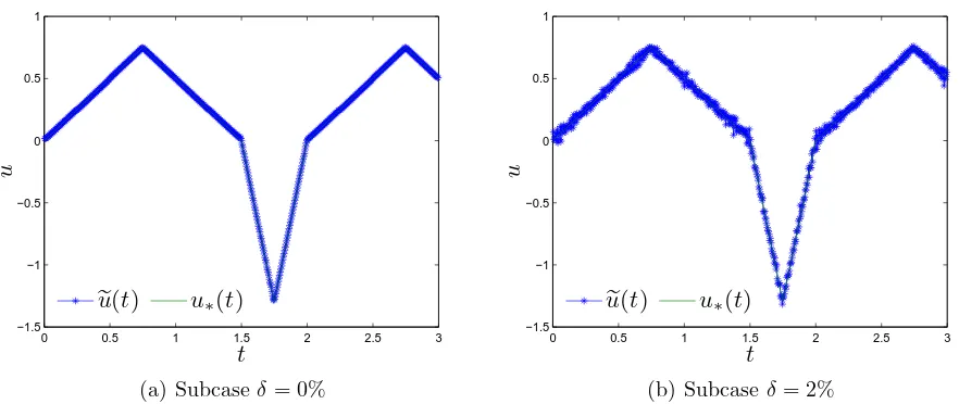
5. Numerical Experiments
Numerical experiments were produced for the problem (4.1) withl= 1,T = 3 = 3l >2l,p= 3 and µ= 1. As a terminal target state f = (f0(x), f1(x)) we choose
f0(x) =u∗(3l−x)−u∗(l+x) +u∗(l−x), 0< x < l,
f1(x) =u′∗(3l−x)−u∗′(l+x) +u′∗(l−x), 0< x < l, (5.1)
where
u∗(t) =
3l/4− |t−3l/4|, 0< t <3l/2,
3√3 (|t−7l/4| −l/4), 3l/2< t <2l, 3l/4− |t−11l/4|, 2l < t <3l.
Note that at first we chose control u∗(t) such that u∗ ∈ JHR(A∗). After that using explicit
expressions for the solution of boundary value problem (4.1) we defined targetf =Au∗, so according to corollary1it means thatu∗(t) is the solution to (2). Plots ofu∗(t) andf(x) are shown at Figure1 and Figure 2respectively.
0 0.5 1 1.5 2 2.5 3
−1.5 −1 −0.5 0 0.5 1
t
u
u
∗(t)
Figure 1. Plot of the exact controlu∗(t)
Approximate operator An was built similar to [18] using three-layer explicit difference scheme
on a uniform grid with M nodes on segment [0, l] and N nodes on [0, T]. Approximate terminal state fn was produced by discretization of functions (5.1) and by adding random noise of fixed
level δ = kfn−fdkF/kfdkF, where fd is discretized function (5.1). The Table 1 presents some
relative errorsǫ=kun−u∗kH/ku∗kH (whereH=L3(0,1)) of finding control u∗(t) by the method, depending on grid parameters M, N and noise level δ in target state. Some typical plots of approximate controls un(t) are presented at Figure3 and Figure4.
0 0.2 0.4 0.6 0.8 1 0
0.2 0.4 0.6 0.8 1 1.2 1.4 1.6 1.8
x
f
0
f0 (x)
(a) Plot off0 (x)
0 0.2 0.4 0.6 0.8 1 −4
−2 0 2 4 6 8
x
f
1
f1 (x)
(b) Plot off1 (x)
Figure 2. Plot of the exact terminal statef(x)
N M δ ǫ
150 50 0% 6.67% 155 50 0% 4.27% 150 50 8% 20.3% 155 50 8% 19.9% 300 100 0% 3.21% 310 100 0% 2.08%
300 100 4% 19%
310 100 4% 11.5% 600 200 0% 1.16% 620 200 0% 0.97% 600 200 2% 12.6% 620 200 2% 5.11%
Table 1. Relative errorsǫ=kun−u∗kH/ku∗kH of the method
of our method are its universality, the possibility of applying to a wide class of ill-posed problems in Banach spaces and also the existence of a theoretical base in the form of assumptions B1–B7.
6. Conclusion
0 0.5 1 1.5 2 2.5 3 −1.5
−1 −0.5 0 0.5 1
t
u
e
u(t) u∗(t)
(a) Subcaseδ= 0%
0 0.5 1 1.5 2 2.5 3 −1.5
−1 −0.5 0 0.5 1
t
u
e
u(t) u∗(t)
(b) Subcaseδ= 8%
Figure 3. Plots of approximate solution eu(t) = un(t) in comparison to exact solution u∗(t) in the case
N = 155,M = 50
REFERENCES
1. Adams R. A., Fournier J. J. F.Sobolev Spaces.Amsterdam: Elsevier, 2003. 320 p.
2. Bakushinskii A. B. Methods for solving monotonic variational inequalities, based on the principle of iterative regularization.USSR Computational Mathematics and Mathematical Physics, 1977. Vol. 17, No. 6. P. 12–24.
3. Bakushinsky A., Goncharsky A.III-Posed Problems: Theory and Applications.Dordrecht: Kluwer Aca-demic Publishers, 1994. 258 p.DOI: 10.1007/978-94-011-1026-6
4. Brezis H.Functional Analysis, Sobolev Spaces and Partial Differential Equations.New York: Springer, 2011. 599 p.DOI: 10.1007/978-0-387-70914-7
5. Cioranescu I. Geometry of Banach Spaces, Duality Mappings and Nonlinear Problems. Dordrecht: Kluwer Academic Publishers, 1990. 260 p.DOI: 10.1007/978-94-009-2121-4
6. Dryazhenkov A. A., Potapov M. M. Constructive observability inequalities for weak generalized solutions of the wave equation with elastic restraint.Comput. Math. Math. Phys., 2014. Vol. 54, No. 6. P. 939–952. DOI: 10.1134/S0965542514060062
7. Dunford N., Schwartz J. T.Linear Operators. Part I: General Theory.New York: Interscience Publishers, 1958. 872 p.
8. Ekeland I., Temam R.Convex Analysis and Variational Problems.Amsterdam: North-Holland Publish-ing Company, 1976. 394 p.DOI: 10.1137/1.9781611971088
9. Ekeland I., Turnbull T. Infinite-Dimensional Optimization and Convexity.Chicago: The University of Chicago Press, 1983. 174 p.
10. Engl H. W., Hanke M., Neubauer A.Regularization of Inverse Problems. Dordrecht: Kluwer Academic Publishers, 1996. 322 p.
11. Il’in V. A., Kuleshov A. A. On some properties of generalized solutions of the wave equation in the classes
LpandW
1
p forp≥1.Differ. Equ., 2012. Vol. 48, No. 11. P. 1470–1476.DOI: 10.1134/S0012266112110043
12. Ivanov V. K. On linear problems that are not well-posed. Soviet Mathematics Doklady, 1962. Vol. 3. P. 981–983.
13. Kantorovich L. V., Akilov G. P. Functional Analysis. Oxford: Pergamon Press, 1982. 604 p. DOI: 10.1016/C2013-0-03044-7
14. Krein S. G. Linear Equations in Banach Spaces. Boston: Birkh¨auser, 1982. 106 p. DOI: 10.1007/978-1-4684-8068-9
0 0.5 1 1.5 2 2.5 3 −1.5
−1 −0.5 0 0.5 1
t
u
e
u(t) u∗(t)
(a) Subcaseδ= 0%
0 0.5 1 1.5 2 2.5 3 −1.5
−1 −0.5 0 0.5 1
t
u
e
u(t) u∗(t)
(b) Subcaseδ= 2%
Figure 4. Plots of approximate solution eu(t) = un(t) in comparison to exact solution u∗(t) in the case
N = 620,M = 200
16. Morozov V. A. Regularization of incorrectly posed problems and the choice of regularization param-eter. USSR Computational Mathematics and Mathematical Physics, 1966. Vol. 6, No. 1. P. 242–251. DOI: 10.1016/0041-5553(66)90046-2
17. Phillips D. L. A technique for the numerical solution of certain integral equations of the first kind. J. ACM, 1962. Vol. 9, No. 1. P. 84–97.DOI: 10.1145/321105.321114
18. Potapov M. M. Strong convergence of difference approximations for problems of boundary control and observation for the wave equation.Comput. Math. Math. Phys., 1998. Vol. 38, No. 3. P. 373–383. 19. Potapov M. M. A stable method for solving linear equations with nonuniformly perturbed operators.
Dokl. Math., 1999. Vol. 59, No. 2. P. 286–288.
20. Riesz F., Sz.-Nagy B.Functional Analysis. London: Blackie & Son Limited, 1956. 468 p.
21. Scherzer O., Grasmair M., Grossauer H., Haltmeier M., Lenzen F.Variational Methods in Imaging.New York: Springer, 2009. 320 p.DOI: 10.1007/978-0-387-69277-7
22. Schuster T., Kaltenbacher B., Hofmann B., Kazimierski K. S.Regularization Methods in Banach Spaces.
Berlin: De Gruyter, 2012. 283 p.
23. Tikhonov A. N. Solution of incorrectly formulated problems and the regularization method.Soviet
Math-ematics Doklady, 1963. Vol. 4, No. 4. P. 1035–1038.
24. Tikhonov A. N., Arsenin V. Y.Solution of Ill-posed Problems.Washington: Winston & Sons, 1977. 258 p. 25. Tikhonov A. N., Leonov A. S., Yagola A. G. Nonlinear Ill-posed Problems. London: Chapman & Hall,
1998. 386 p.
26. Zuazua E. Propagation, observation, and control of waves approximated by finite difference methods.