Commodity Prices in the Presence of
Inter-commodity Equilibrium Relationships
∗Jaime Casassus
Pontificia Universidad Catolica de Chile
Peng (Peter) Liu
Cornell University
Ke Tang
Renmin University of China Revised: May 2009
∗
Please address any comments to Jaime Casassus, Escuela de Ingenieria, Pontificia Universidad Catolica de Chile, email: [email protected]; Peng Liu, Cornell University, 465 Statler Hall, Ithaca, NY, 14850, email: [email protected]; Ke Tang, Mingde Building, Hanqing Advanced Institute of Economics and Finance, Renmin University of China, Beijing, 100872, email: [email protected]. Casassus acknowledges financial support from FONDECYT (grant 1070688). Liu acknowledges the financial support from The School of Hotel Administration at Cornell University. Most of the work was completed when Tang was at Cambridge University and JP Morgan & Chase Co. Any errors or omissions are the responsibility of the authors.
Commodity Prices in the Presence of Inter-commodity Equilibrium Relationships
Abstract
This paper shows that the long-term co-movement among commodities is driven by economic re-lations, such as, production, substitution or complementary relationships. We refer to these as inter-commodity equilibrium (ICE) relationships. An ICE relation implies a long-term source of co-movement that is not captured by traditional commodity pricing models. In particular, we find a cross-commodity feedback effect where the convenience yield of a certain commodity is determined, among other things, by the prices of related commodities. We test this prediction in a multi-commodity model that dis-entangles a short-term source of co-movement from the long-term ICE component. We estimate the model for the heating oil - crude oil and for the WTI - Brent crude oil pairs. We find that ICE relations are pervasive and significant, both, statistically and economically. The correlation structure implied by our model matches the upward sloping curves observed in the data. The ICE relationship considerably reduces the long-term volatility of the spread between commodities which implies lower spread option prices.
Keywords: Inter-commodity equilibrium (ICE), commodity prices, convenience yields, cross-commodity feedback effects, correlation structure, spread options.
1
Introduction
Commodity markets have experienced dramatic up-and-down movements in a relatively short time period. Closest-to-maturity crude-oil futures have increased from almost $50 per barrel in January 2007 to $147 per barrel in July 2008, the highest level in history since it is traded in NYMEX. Surprisingly, only 5 months later, the oil price drop to almost $30 per barrel. The energy sector, agricultural commodities and industry metals have experienced similar patterns. While academics and policy makers are still trying to understand the causes, the following stylized facts, among others have been reinforced after the turmoil: 1) commodity prices are volatile, 2) spot and futures prices are mean-reverting, and 3) prices of multiple commodities co-move. These characteristics play a critical role in modeling financial contingent claims on commodities.
Since Keynes (1923), many scholars have studied the stochastic behavior of individual com-modities. However, relationships between multiple commodities have received little attention in theoretical modeling and commodity-related contingent-claim pricing. These cross-commodity re-lationships imply that two or several commodities share an equilibrium that links prices in the long run. We refer to these long-term connections as inter-commodity equilibrium (ICE) ships. Examples of economic ICE relationships between commodities include production relation-ship where upstream commodity and downstream commodity are tied in a production process, and substitute/complementary relationships where two commodities serve as substitute/complement in consumption and/or production.
The existence of ICE usually indicates long-term co-movement among commodity prices. Tem-porary deviation from the ICE (because of demand and supply imbalances caused by macro-economic factors and inventory shocks, etc.) will be corrected over the long-run. This implies that co-movement exists not only in spot prices, but also in expected prices, which are determined by convenience yield and risk premia, among others. The presence of ICE suggests for example, that the convenience yield of one commodity is affected by the spot price of other commodities.
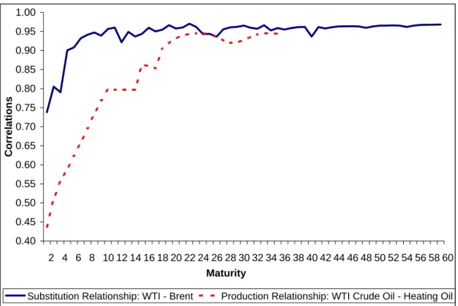
Figure 1 shows the correlation structure of weekly futures returns for the heating - crude oil and for the WTI - Brent crude oil pairs between 1986.07 to 2009.04. These ICE commodity pairs follow a production and a substitute relationship, respectively. The plot shows upward sloping correlation
structures for both commodity pairs. Prices are tied by the long-term ICE relationship which translates into higher long-term correlations. Interestingly, tradicional commodity pricing models, such as correlated versions of the Gibson and Schwartz (1990) (hereafter GS) and the Casassus and Collin-Dufresne (2005) (hereafter CCD) models, are unable to match this evidence. Moreover, the correlation structure is crucial for the pricing of commodity spread options, which suggest that the option prices implied by the traditional models have strong biases. We propose a reduced-form model that allows for a flexible correlation structure that matches the pattern observed in the data. We find that for long-maturity spread options, the prices implied by our model are lower than the ones predicted by the traditional models, because the higher long-term correlation reduces the volatility of the spread. We show that the opposite occurs for short-maturity options.
In econometrics, long-term equilibrium relationships (such as ICEs) are usually expressed in the format of cointegration or Error Correction Models (ECMs). Engle and Granger (1987) shows that the ECM is identical with a cointegration model if the underlying time series are non-stationary. An ECM predicts that the adjustment in a dependent variable depends not only on the explanatory variables but also on the extent to which an explanatory variable deviates from the equilibrium (refer to Banerjee, Dolado, Galbraith, and Hendry 1993). Many scholars have empirically studied the cointegration/ECM relationships among commodities. Among them, Pindyck and Rotem-berg (1990) tests and confirm the existence of a “puzzling” phenomenon - the prices of raw com-modities have a persistent tendency to move together. Ai, Chatrath, and Song (2006) documents that the market-level indicators such as inventory and harvest size explain a strikingly large portion of price co-movements. Malliaris and Urrutia (1996) documents a long-term cointegration among prices of agricultural commodity futures contracts from CBOT. Girma and Paulson (1999) finds a cointegration relationship in petroleum futures markets. Recently, Paschke and Prokopczuk (2007) and Cortazar, Milla, and Severino (2008) have studied the statistical relationship among commodi-ties in a multi-commodity affine framework using futures prices. However, none of these models give an economic foundation about which type of assets and why prices of multiple commodities move together through time. To the best of our knowledge no previous research have looked at the patterns of co-movements among multiple commodities under ICE relationships.
of commodity prices. This literature documents the following stylized facts for single commodities: the existence of a stochastic convenience yield (e.g. GS and Brennan 1991), mean-reversion in prices (e.g. Bessembinder, Coughenour, Seguin, and Smoller 1995, and Schwartz 1997), seasonality (e.g. Richter and Sorensen 2002), time-varying risk-premia (e.g. CCD) and stochastic volatility (e.g. Trolle and Schwartz 2009).
Our paper is organized as follows. Section 2 identifies three economic inter-commodity equilib-rium (ICE) relationships and provide examples of such relationships. Section 3 solves an economic model for the case of two commodities that have a production relationship and generates an en-dogenous cross-commodity feedback effect. Guided by the economic model, section 4 develops an empirical model that captures the co-movement among prices (and price dynamics) in a multi-commodity system. We also show that our model is an extension of the “maximal” affine model to a multi-assets case. Section 5 describes the estimation of the model and shows the estimation results. Section 6 presents the valuation of spread options under our multi-commodity framework, and section 7 concludes.
2
Inter-Commodity Equilibrium (ICE) Relationships
The co-movement of commodity prices and the existence of inter-commodity equilibrium (ICE) relationships are pervasive in the economy. Examples of the economic ICE relationships between different commodities include, but are not restricted to the following cases:
Production Relationships
One commodity can be produced from another commodity when the former is the output of a production process that uses the other commodity as an input factor. For example, the petroleum refining process “cracks” crude oil into its constituent products, among which heating oil and gasoline are actively traded commodities on the New York Mercantile Exchange along with crude oil. Spread futures and spread options, such as the 3:2:1 crack spreads (the purchase of three crude oil futures with the simultaneous sales of two unleaded gasoline futures and one heating oil future), are widely used by refiners and oil investors to lock in profit margins. A similar production
relationship can be found in the soybean complex. Soybeans can be crushed into soybean meal and soybean oil. The three commodities in the complex are traded separately on the Chicago Board of Trade. By analogy to the crack spread, the crush spread is also a actively traded derivative. Not all productionlinked commodities have spread derivatives established for trading. Aluminum -Aluminum Alloy and corn - ethanol are other examples of the production-linked ICE relationships without spread trading.
Substitute Relationships
A substitute relationship exists when two traded commodities are substitutes in consumption. Crude oil and natural gas are commonly viewed as substitute goods. Competition between natural gas and petroleum products occurs principally in the industrial and electric generation sectors. According to the EIA Manufacturing Energy Consumption Survey (Energy Information Adminis-tration 2002), approximately 18 percent of natural gas usage can be switched to petroleum products. Other analysts estimate that up to 20 percent of power generation capacity is dual-fired. West Texas Intermediate (WTI), a type of crude oil often referenced in North America, and Brent crude oil from the North Sea, are commonly used as benchmarks in oil pricing and the underlying commod-ity of NYMEX oil futures contracts. WTI and Brent crude represent an example of a substitute relationship. Recently NYMEX started to trade WTI-Brent spread option. Corn and soybean meal serve as substitute cattle feeds. Ethanol - petroleum products are potentially competitive products.
Complementary Relationships
A complementary relationship exists when two commodities share a balanced supply or are com-plementary in consumption and/or production. Let’s consider the case of gasoline and heating oil. If the gasoline price increases dramatically, and crude oil is cracked to supply gasoline, this process also produces heating oil and may result in a drop in the price of heating oil. The relationship between these two commodities is one of complementarity. On the other hand, lead, tin, zinc and copper are often smelted from paragenesis mineral deposits. The equilibrium assemblage of mineral phases gives those industrial metals a natural relationship in supply. Crude oil and minerals from industrial metals are generally concentrated in developing countries whose economy relies heavily on commodity exports. In addition, industrial metals are seldom used in their pure forms. They
find most applications in the form of alloys. For example, the principal alloys of tin are bronze (tin and copper), soft solder (tin and lead), and pewter (75% tin and 25% lead). Two-thirds of nickel stocks are used in stainless steel, an alloy of steel. In 1998, 48% of zinc was applied as zinc coatings, jointly used with aluminium.
The three above-mentioned economic ICE relationships can be present simultaneously among commodities. For example, while complementarity exists between gasoline and heating oil, some substitutability is also at play. In the following section we present a structural model for the production relationship and the implication of the ICE relation in the prices dynamics.
3
The Economic Model
Commodity prices link two interconnected markets: the cash (or futures) market and the inventory market. Immediate ownership of a physical commodity offers some benefit or convenience that is not provided by futures ownership. This benefit, in terms of a rate, is called the “convenience yield” (see Brennan 1991, and Schwartz 1997). The “Theory of Storage” of Kaldor (1939), Working (1948) and Telser (1958), predicts that the return from purchasing a commodity and selling it for delivery (using futures) equals the interest forgone less the convenience yield. The convenience yield is attributed to the benefit of protecting regular production from temporary shortages of a particular commodity or by taking advantage of a rise in demand and price without resorting to a revision of the production schedule.
The traditional presentation of the Theory of Storage proposes thata “high” convenience yield is associated with a “high” spot price (see Pindyck 2001). If we only consider the market for any single commodity, the statement indicates: 1) the convenience yield is an increasing function of the spot price; or 2) there is a positive correlation ofincremental changes between the spot price and the convenience yield. This paper extends the Theory of Storage by introducing a third interpretation, i.e., 3) a high level of convenience yield of a particular commodity corresponds to a highprice-level difference between relative commodities in an ICE relationship. The first two interpretations have been studied by several authors. For example, CCD explicitly model the positive dependence of the convenience yield on the spot price and the instantaneous positive correlation between the spot
price and the convenience yield. However, the third interpretation has received little attention so far.
To motivate the importance of the third interpretation, let’s give an example where interpre-tation 1) is violated, however it is consistent with interpreinterpre-tation 3). Consider a system of two commodities, heating oil and crude oil, where there is a production relationship in long-term equi-librium. Assume at time 0 that heating/crude oil are $20/$15, respectively, while at time 1 they move to $22/$21, respectively. First, let’s consider the convenience yield of heating oil. If we look only at the heating oil market, since the heating oil is more expensive at time 1, we expect to have a greater convenience yield at time 1 than at time 0. However, if we look at both markets –heating oil and crude oil– together, we should expect the convenience yield of heating oil to be smaller at time 1 than at time 0. Indeed, since heating oil is only refined from crude oil, a high spread between heating and crude oil at time 0 (i.e., the high production profit), indicates that the refining capability cannot satisfy the strong demand for heating oil. Thus heating oil is relatively scarce and should have relatively higher convenience yields than at time 1 when the heating oil is very likely in abundance. Thus, the relative prices of heating and crude oil do influence the convenience yield of the commodities.
The dependence of the convenience yield of a certain commodity on other commodities is not part of the traditional Theory of Storage. We provide the intuition in a simple production equi-librium highlighting the ICE relationship between crude oil an heating oil. This economy builds on the single commodity equilibrium models of Casassus, Collin-Dufresne, and Routledge (2008) and Routledge, Seppi, and Spatt (2000) and is similar in spirit to the cross-commodity model of Routledge, Seppi, and Spatt (2001).
To formalize the economic intuition developed above, we consider a continuous-time production economy with an infinite time horizon. This economy has a capital sector (Kt) and two storable
commodity sectors: crude oil (Q1,t) and heating oil (Q2,t). A representative agent derives utility
from the following two consumption goods: heating oil and the standard consumption good from the capital sector that is used as the numeraire. The representative agent maximizes expected log utility with respect to consumption of capital (CK,t), consumption of heating oil (C2,t) and demand
for crude oil (q1,t):1 sup {CK,t,C2,t,q1,t} ∈ A E0 Z ∞ 0 e−θ t(φlog (CK,t) + (1−φ) log (C2,t))dt (1)
where A is the set of admissible strategies. The optimization problem is subject to the following processes that describe the dynamics of the stocks of capital, crude oil and heating oil, respectively:
dK = (α K−CK)dt+σKK dWK (2)
dQ1 = −q1dt (3)
dQ2 = (γ log(q1)Q2−C2)dt (4)
The production rate of heating oil is an increasing function of the input quantityq1 that flows from the crude oil stocks. For simplicity, we assume that this rate has a logarithmic form and that crude oil can be used only as an input to the heating oil technology. We assume that the capital sector has a constant return-to-scale technology. Finally, following Cox, Ingersoll Jr., and Ross (1985), we assume that the output of the capital sector is stochastic. Uncertainty in the economy is captured by the Brownian motionWK and σK is the volatility of output returns.
As expected, the representative agent optimally consumes a constant fraction of capital (CK =
θ K), a constant fraction of heating oil (C2 = θ Q2), and demands a constant rate of crude oil (q1 = θ Q1).2 The market-clearing prices are determined by marginal utility indifference. The commodity prices correspond to the amount of capital the representative agent is willing to give for an extra unit of commodity (i.e. the shadow price). In this simple economy the equilibrium prices for crude oil (S1) and heating oil (S2) are given by:
S1 = 1−φ φ γ θ K Q1 and S2 = 1−φ φ K Q2 (5)
The equilibrium convenience yields are related to the marginal productivity of each commodity in the economy (see Casassus, Collin-Dufresne, and Routledge 2008). A relevant prediction for us is that the convenience yield of heating oil (δ2) is a time-varying and increasing function of the crude
1
These variables are all time dependent. Hereafter, we drop this dependance throughout the paper to simplify the notation.
2
oil stocks:3 δ2 = γlog (θ Q1) = γ log 1−φ φ γK −log (S1) (6)
Furthermore, since the crude oil price (S1) is decreasing in its stock (Q1), equation (6) shows that the heating oil convenience yield is a decreasing linear function of the (log) crude oil price plus another risk factor that in this case is log(K). Higher crude oil inventories imply lower crude oil prices and higher heating oil convenience yields. The intuition is the following. Since the production rate of heating oil is increasing in the crude oil inventories, more inventories of crude oil today imply more inventories and lower prices of heating oil in the near future. The heating oil spot price is expected to decrease, which in this model implies lower futures prices.4
This inter-commodity relationship exists because crude oil is an input for heating oil produc-tion. The model can be extended in several ways, but as long as the ICE relationship exists, the crude oil price will influence the heating oil price dynamics (through the heating oil convenience yield). Appendices B.1 and B.2 provide structural models for the substitute and complementary relationship respectively, which show a similar phenomenon to the one mentioned above.
In summary, if an ICE relationship exists among commodities, the structural models predict that the dynamics of a certain commodity is partly determined by the behavior of related commodities. In particular, the structural ICE model suggests that the inter-commodity connection is through the convenience yields. In the next section, we propose a reduced-form model with the interdependence of the convenience yield on other commodity prices that is in line with our theoretical prediction.
4
The Empirical Model
This section introduces a reduced-form model that is consistent with the stylized facts from ICE commodities (i.e. upward sloping correlation structure, stochastic convenience yields, mean-reversion, etc.). Our multi-commodity model is parsimonious in the sense of “maximal” affine
3In this simplified economy, the convenience yield of crude oil is zero. 4
Indeed, in this economy the heating oil risk-premium is constant (σ2K). The interest rate is also constant (r= α−σ2K), thus all the action in the expected spot price is given by the time-varying convenience yield.
models.5 We prefer to build a maximal model in order to avoid the risk of model mis-specification. Furthermore, we distinguish two sources of co-movement across commodities: 1) a short-term effect associated to the correlation of commodity prices, and 2) a long-term effect that is a consequence of the ICE relationship. The long-term effect manifests in that the dynamics of one commodity is a function of the other commodities in the economy. In particular, we choose a representation in such a way that the long-term effect is present, because the convenience yield of a particular commodity depends on the other commodities.
4.1 The Data-generating Processes
Assume there are ncommodities in the system, in which the commodities have ICE relationships. Denote
xi= log(Si) for i= 1, . . . , n (7)
where Si is the spot price of commodity i. Under the physical measure (P), we assume the (log) spot prices follow Gaussian processes
dxi = (µei−δi)dt+σidWi for i= 1, . . . , n (8)
where δi is the convenience yield of commodity i, and µei and σi are constants. Here, Wi (i =
1, . . . , n) are correlated Brownian motions. Motivated by our structural framework above, we propose a specification where the convenience yield of commodity i, δi, is a function of the spot
prices of then commodities in the economy. Furthermore, there are alsonextra latent factors,ηj
(j = 1, . . . , n), affecting the nconvenience yields. For simplicity, we consider anaffine relationship among the convenience yields and the risk factors. Therefore,
δi =− n X j=1 bi,jxj +ηi− n X j=1,i6=j ai,jηj (9)
5An affine structure is the standard framework for commodity pricing reduced-form models (see for example, GS and Schwartz 1997). See Dai and Singleton (2000) and CCD for the definition of “maximal” in this context.
wherebi,j andai,j are constants. The latent factorsη’s follow mean-reverting processes of the form,
dηi= (θei(t)−kiηi)dt+σn+idWn+i for n= 1, . . . , n (10)
Here,θei(t) =χei+ωi(t), whereχeiis a constant andωi(t) is a periodical function ontto capture the
seasonality of commodity futures prices (if any). Refer to Richter and Sorensen (2002) and Geman and Nguyen (2005) for a similar setup on the seasonality of the convenience yields. Following Harvey (1991) and Durbin and Koopman (2001), we specify ωi(t) as:
ωi(t) = L X
l=1
(sc,li cos 2π l t+ss,li sin 2π l t) (11)
Letting Y = (x1, . . . , xn, η1, . . . , ηn)> denote the 2n factors driving the system of n commodity
prices, our model can be rewritten in a vector form,
dY = e U(t) + ΨY dt+dβ (12) whereUe(t) = (µe1, . . . ,µen,θe1(t), . . . ,θen(t))>, and Ψ = B A 0 K with B = b1,1 b1,2 · · · b1,n b2,1 b2,2 . .. b2,n .. . . .. . .. ... bn,1 bn,2 · · · bn,n , A= −1 a1,2 · · · a1,n a2,1 −1 . .. a2,n .. . . .. . .. ... an,1 an,2 · · · −1 ,K = −k1 0 · · · 0 0 −k2 . .. 0 .. . . .. . .. ... 0 0 · · · −kn
In equation (12), β = (σ1W1, . . . , σ2nW2n)> is a scaled Brownian motion vector with covariance
matrix Ω = {ρi,jσiσj} for i, j= 1,2, . . . ,2n, where ρi,jdt is the instantaneous correlation between
the Brownian motion increments dWi and dWj.
Our model nests several other classical models:
1. If bi,k = 0 and ai,k6=i = 0 (i = 1, . . . , n;k = 1, . . . , n), our model reduces to correlated GS
models on commodities.
2. Ifbi,k6=i = 0 and ai,k=6 i = 0 (i= 1, . . . , n;k= 1, . . . , n), our model reduces to correlated CCD
The correlated GS and CCD models correspond to the GS and CCD models when the spot prices and convenience yields across commodities are correlated. The correlated version of the models are more flexible than the original models and later will be considered as benchmarks for our model.
4.2 Co-movement in Commodity Prices
A natural way of extending the traditional single commodity-pricing models to a multi-asset frame-work, is to assume that the shocks of the factors are correlated. Indeed, if the objective is to study the valuation of derivatives or the portfolio selection problem in a multi-commodity framework, then correlated factors need to be considered. However, these correlations only generate a short-term source of co-movement in commodity prices. This type of co-movement fails to recognize the long-term effect that exists in the inter-commodity equilibrium relationships. This is the case for the correlated versions of the GS and CCD models.
The proposed empirical model in this paper makes an important distinction between the two components of the co-movement between commodities. In contrast to the short-term effect im-plemented by the instantaneous correlation structure in Brownian motions of different commodity prices, the ICE relationship generates a longer term effect. This long-term source of co-movement is a feedback effect that is mainly at play through the connection between the expected returns of different commodities, i.e. the way a particular commodity impacts the expected return of the other commodities in the economy.6 This cross-commodity feedback effect corresponds to an er-ror correction or the cointegration between different time series in the discrete-time econometric literature.7
In the model, the expected return of xi is
E[dxi] = eµi+ n X j=1 bi,jxj−ηi+ n X j=1,i6=j ai,jηj dt (13) 6
The term “feedback effect” has had different interpretations in the econometrics and finance literature. Here, we borrow the concept from the term-structure literature, that refers basically to the non-diagonal terms of the long-run matrix Ψ. See Dai and Singleton (2000) and Duffee (2002) for more details.
7
The ai,j’s and the bi,j’s (for j 6= i) represent the long-term source of co-movement.8 These
pa-rameters relate the expected return of the commodity i with the price and convenience yield of commodity j. The correlated GS and CCD models set these parameters to zero, therefore they completely ignore the cross-commodity feedback effect.
According to the sign of thebi,j’s, we classify the co-movement between commodity (log) prices
xi and xj (j 6=i) into three classes. That is, if bothbi,j >0 and bj,i > 0, a positive increment of
xi tend to feedback a positive increment onxj, which is in turn likely to strengthen xi by another
positive feedback; hence xi and xj move together. Similarly, ifbi,j <0 andbj,i<0xi andxj move
in opposite directions. Lastly, we have the mixed casesbi,j >0,bj,i<0 andbi,j <0,bj,i>0, where
it is not easy to tell the type of co-movement between the commodity prices.
The covariance matrix Σ(t, T) for the vector of commodity pricesXT conditional onXtis
Σ(t, T) =
Z T t
eΨ(T−u)ΩeΨ>(T−u)du (14)
The covariance is stationary as long as all eigenvalues of the long-run matrix Ψ are negative, which is indeed the case for all the commodity pairs studied in the empirical section. From the definition of the conditional covariance we obtain the conditional price correlation (i.e. the correlation structure),
ρ(t, T)i,j =
Σ(t, T)i,j p
Σ(t, T)i,iΣ(t, T)j,j
for i, j= 1, . . . , n (15)
It is easy to see that whenT →ttheinstantaneous conditional price correlation isρi,j which does
not depend on the long-run matrix Ψ, i.e. limT→tρ(t, T)i,j = ρi,j. This means that in the short
run, the correlation among the factors is an important source of co-movement.
For a longer period of time τ = T −t > 0, the conditional price correlation does depend on Ψ, and it is impacted by the relationship among the commodities. If there is a long-term ICE relationship, it will appear in the a’s and b’s, which in turn affects the long-run matrix Ψ. This dynamics creates another source of co-movement that takes effect at relatively longer horizons.
Figures 5 and 9 show that the cross-commodity feedback effect due to the ICE relationship, does
8
Note from equation (9) that if ai,j 6= 0, then the convenience yield for both commodities i and j share the
play an important role in explaining the co-movement of commodity prices. The figure shows that by neglecting the cross-commodity parameters, the GS and CCD models impose strong restrictions on the correlation structure. The cross-commodity feedback effect is necessary to match the upward sloping correlation structure in the data.
4.3 Futures Pricing
Assuming a constant risk premium for each factor, the risk-neutral process can be expressed as follows:
dβQ = Πdt+dβ (16)
where Π = (πx,1, . . . , πx,n, πη,1, . . . , πη,n)> is the risk premium vector. A constant risk premium
restricts the long-run behavior (i.e. the Ψ matrix) to be the same under both, risk-neutral and physical measures, but reduces considerably the number of parameters to estimate.
The drift partU(t) under the risk neutral measure can be specified as,U(t) =Ue(t)−Π, hence,
dY = (U(t) + ΨY)dt+dβQ (17)
where βQ = (σ
1W1Q, . . . , σ2nW2Qn)> and U(t) = (R, L(t))
>
with R = (rf − 12σ12, . . . , rf − 12σn2)>, L(t) = (θ1(t), . . . , θn(t))>, θi(t) = χi+ωi(t) and χi = χei −πη,i. We assume a constant interest
risk-free rate rf to keep the model simple.9
The following proposition shows the futures prices for each commodity i:
Proposition 1 Let Fi,t(Yt, T) be the ith commodity futures price maturing in τ =T −t periods.
In the model setup (17), the futures prices are determined by
log(Fi,t(Yt, t+τ)) =mi(τ) +Gi(τ)Yt for i= 1, . . . , n (18)
where mi(τ) = Z τ 0 Gi(u)U + 1 2Gi(u) ΩGi(u) > du
G(τ) = exp(Ψτ)
where Gi(τ) denotes the ith row of the G(τ) matrix.
Proof See Appendix D.1.
4.4 “Maximal” Affine Model in a Multi-commodity System
Duffie and Kan (1996), Duffie, Pan, and Singleton (2000) and Dai and Singleton (2000) propose a “maximal” canonical form for affine multi-factor model of the form:
xi =αi0+ψiYb
b
Y , (19)
where xi denotes the (log) value of the ith asset, ψi
b
Y is a 1×m constant row vector and α i
0 is a constant. Yb is anm×1 column vector of latent state variables that follow mean-reverting Gaussian
diffusion processes under the risk-neutral measure,
dYb =−ΛY dtb +dWQ
b
Y (20)
where Λ is a lower triangular matrix and WQ
b
Y is a vector of independent Brownian motions. The
above-mentioned model is “maximal” in the sense that, conditional on observing the single asset, the model offers the maximum number of identifiable parameters (c.f. Dai and Singleton 2000, and CCD).
In order to use this model into a multi-commodity system, we have to extend it in two ways. First, the above maximal model is only suitable for a single asset, thus we need to extend the model to a canonical affine representation for multiple assets. We hence define the maximal model for multiple assets as follows:
In a system of nassets which are governed by m factors, a model for the system is “maximal”
if and only if every single asset in the system is modeled by an m-factor maximal model as defined
in Dai and Singleton (2000):
where X = (x1, . . . , xn)> represent the n assets which are governed by Yb in equation (20). Here, ψ b Y = (ψ 1 b Y, . . . , ψ n b Y) > is an n×m matrix and ψ 0 = (ψ01, . . . , ψn0)> is an n×1 vector.
Thus a simple combination of maximal models for single commodities does not necessarily form a maximal model for a multi-commodity system. For example, the CCD model is maximal for single commodities, but is not maximal in a multi-commodity system. The previous section shows that an extended version of the CCD model is nested in our model and hence is not maximal, because this model restricts some parameters in the expected return of the factors to be zero. These constraints considerably influence the joint long-run behavior of the commodities and are directly related to the ICE relationship.
Second, the above maximal model only allows a constantψ0, however, many commodity prices are subjective to seasonal movements. Thus, we need to extend the maximal model by letting ψ0 be time-varying. The extended model for multiple assets is:
X = ψ0(t) +ψYbY ,b (22)
dYb = −ΛY dtb +dWQ
b
Y (23)
whereψ0(t) = (ψ01(t), ψ20(t), . . . , ψn0(t))> is ann×1 vector,ψi0(t) =αi0+$0i(t), and where$0i(t) is a periodical function.
To address the maximal model for multiple assets in an ncommodities system governed by 2n factors, we specify X as the n×1 vector of (log) spot commodity prices, Λ in (20) as a 2n×2n lower triangle matrix and WQ
b
Y as a 2n×1 vector of independent Brownian motions.
Following CCD we now show that for the multi-commodity maximal model, the convenience yield vector ∆ = (δ1, . . . , δn)>is an affine function of the state variablesYb. The absence of arbitrage
implies that under the risk-neutral measure (Q) the drift of the spot price of the ith commodity must follow
EQt[dSi] = (rf−δi)Sidt for i= 1, . . . , n (24)
∆ implied by our model, ∆ = rf1n− EQt[dV] +12(Var Q t[dx1], . . . ,VartQ[dxn])> dt = rf1n+ψYbΛYb − 1 2diag(ψYbψ > b Y) (25)
where VarQt(.) denotes the variance under the risk-neutral measure, and 1n is an n×1 column
vector with all elements equal to 1.
In order to show that our empirical model from the beginning of this section is indeed maximal, we first introduce an intermediate representation that allows us to show that our model and the one presented in equations (22)-(23) are equivalent. The intermediate representation rotates the state vector Yb to state variables that have a better economic meaning: the (log) spot prices and
the convenience yields of the n commodities. Eventually, we could have included m−2n extra latent state variables in the intermediate representation, but as it will become clear later, a 2n -factor model is enough to capture the joint dynamics of a system of n commodities.10 Thus, we set m= 2n. Proposition 2 formalizes the intermediate representation.
Proposition 2 Assume 2n factors driving the dynamics of the futures prices of n commodities, as in equations (22)-(23). The maximal model under the risk-neutral measure can be presented
equivalently by an affine model where the state variables are the log spot prices xi and convenience
yields δi (i= 1, . . . , n). The dynamics of the new state vector Y = (x1, . . . , xn, δ1, . . . , δn)> is:
dY = (U(t) + ΨY)dt+dβQ Y (26) where U(t) = R, L(t)>, Ψ = 0 −In×n A B and β Q
Y is a scaled Brownian motion vector with
covariance matrixΩ. Then×1 vectorsRandL(t)and the n×nmatricesA,B andΩare specified in Appendix D.2.
Proof By writing equations (22) and (25) together, we have Y = X ∆ = ψ0(t) ψc + ψ b Y ψ b YΛ Y ,b (27) where ψc = rf1n− 12diag(ψYbψ> b
Y). Equation (27) shows that the intermediate representation, Y,
is an invariant transformation ofYb (see Dai and Singleton 2000). This transformation rotates the
state variables, but all the initial properties of the model are maintained, that is, the resulting model is still a maximal affine 2n-factor Gaussian model. Furthermore, we apply Itˆo’s lemma to obtain the specific relationships between the model parameters specified in the proposition and those specified in equations (22)-(23). Appendix D.2 shows the derivation in a greater detail.
An important corollary of Proposition 2 is that, in a maximal model, thedriftof the convenience yield of a certain commodity depends on other commodity spot prices. This is consistent with the structural model in section 3 (for example, see equation (6)).
Now we are ready to show that our model is maximal. The next proposition formalizes this.
Proposition 3 The maximal model specified in Proposition 2 is equivalent with our model in (17).
Proof Equation (9) shows that the convenience yield vector is ∆ = −B X −A η, where η = (η1, . . . , ηn)> is the vector of latent state variables that follow the dynamics in (10). Thus, we find
the following invariant transform from Y toY:
Y = X η = In×n 0 −A−1B −A−1 Y (28)
Similar with Proposition 2, we apply Itˆo’s lemma to compare the parameters in (26) and (28) and show that they are identical. Appendix D.3 shows the derivation in detail.
Proposition 2 and 3 show that our model belongs to the maximal model of multi-commodity sys-tem. Furthermore, it captures the ICE relationship among different commodities. In the following section, we show how to calibrate this model.
5
Estimation
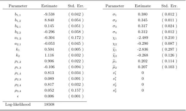
We demonstrate the importance of ICE relationships in futures pricing using a production pair of heating oil and crude oil. A Kalman filtering is applied for implementing our model. Even though our model can be applied to price a system ofn commodities jointly, two commodities are enough to highlight the main characteristics of our model and the intuition behind the results.11 We also estimate a substitution ICE relationship between WTI crude oil and Brent crude oil. The estimation of the WTI-Brent crude oil pair is analogous to the heating and crude oil pair, therefore, we leave the details of the estimation of the substitute case for Appendix C.
5.1 Empirical Method – the Kalman Filter
One of the difficulties of calibrating the model is that the state variables are not directly observable. A useful method for maximum likelihood estimation of the model is addressing the model in a state-space form and to using the Kalman filter methodology to estimate the latent variables.12 The state-space form consists of a transition equation and a measurement equation. The transition equation shows the data-generating process. The measurement equation relates a multivariate time series of observable variables (in our case, futures prices for different maturities) to an unobservable vector of state variables (in our case, the (log) spot prices xi and ηi (i = 1, . . . , n)). The measurement
equation is obtained using a log version of equation (18) by adding uncorrelated noises to take account of the pricing errors.
Suppose that data are sampled in equally separated times tk, k = 1, . . . , K. Denote ∆t =
tk+1−tk as the time interval between two subsequent observations. Let Yk represent the vector of
state variables at timetk. Thus, we can obtain the transition equation,
Yk+1 = (Ψ ∆t+I)Yk+Ue(t) ∆t+wk (29)
11The computational loads increase exponentially for the case of more than two commodities. Furthermore, com-modity pairs are building blocks of any comcom-modity system. Any multi-comcom-modity system can be decomposed into multiple commodity pairs, e.g., the system with three commodities can be priced using no more than 3 pairs of commodities.
12
Hamilton (1994) and Harvey (1991) give a good description of estimation, testing, and model selection of state-space models.
wherewk is a 2n×1 random noise vector following zero-mean normal distributions.
For the measurement equation at time tk, we consider the vector of the log of futures prices
Fk = (F1,k(τ1), . . . , Fn,k(τ1), . . . , F1,k(τM), . . . , Fn,k(τM))>, where τj denotes the time to
maturi-ties.13 The log (n M)×1 vector Fk can be written as,
log(Fk) =m+G Yk+εk (30)
where
m = (m1(τ1), . . . , mn(τ1), . . . , m1(τM), . . . , mn(τM))>,
G = (G1(τ1), . . . , Gn(τ1), . . . , G1(τM), . . . , Gn(τM))>,
and εk is a (n M)×1 vector representing the model errors with its variance covariance matrix Υ.
In order to reduce the number of parameters to estimate, we assume that the standard errors for all contracts are the same. This also reflects the notion that we want our model to price the n commodities andM contracts equally well. Therefore, we define Υ =2InM, whereis the pricing
error of the log of the futures prices and InM is the (n M)×(n M) identity matrix.
5.2 The Data
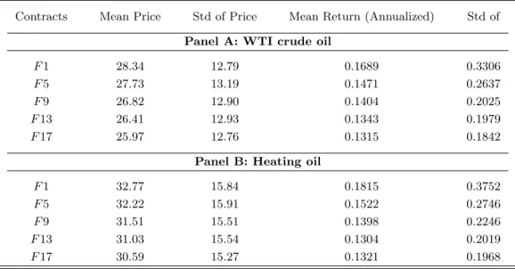
Our data consist of weekly futures prices of West Texas Intermediate (WTI) crude oil and heating oil. The weekly WTI crude oil and heating oil futures are obtained through the New York Mercantile Exchange (NYMEX) for the period from 1995.01 to 2006.02 (582 observations for each commodity). The time to maturity ranges from 1 month to 17 months for these two commodities. We denote F nas futures contracts with roughly n months to maturity; e.g., F0 denotes the cash spot prices and F12 denotes the futures prices with 12 months to maturity. We use five time series —F1,F5, F9,F13, F17– for WTI, crude oil, and heating oil contracts. Table 1 summarizes the data. Note that, in the calibration, we take the risk-free rate as 0.04, which is the average interest rate during these years.
5.3 Empirical Examination of the ICE Relationship
As mentioned before, since WTI crude oil and heating oil are the input and output of the oil refinery firm, they belong to the production relationship and follow an ICE relationship.
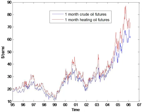
We arbitrarily define crude oil as commodity 1 and heating oil as commodity 2. Figure 2 shows the historical crude and heating oil time series. Crude oil prices does not show seasonality, which is consistent with the literature on oil futures, such as Schwartz (1997). However, heating oil shows quite strong seasonality. This is because in winter, demand for heating oil is typically high, but there are usually not enough facilities existent to store the heating oil; hence, in the winter, heating oil has relatively higher convenience yields. Therefore, winter-maturing futures tends to be higher than those maturing in summer. Since the seasonality of heating oil is in an annual frequency, for simplicity we setL= 1 in equation (11), implying that
ωi(t) =scicos 2π t+ssi sin 2π t (31)
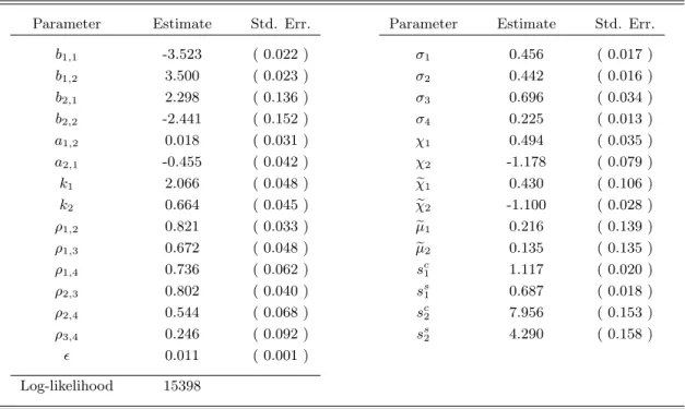
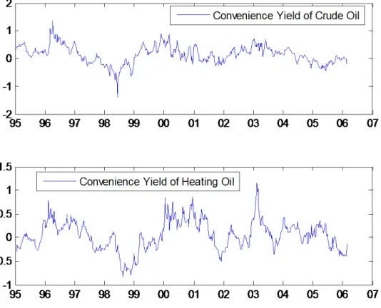
We use the Kalman filter to calibrate our model. Table 2 shows the results. From the model estimation, we see that most parameters are significant. In particular, b1,2 and b2,1 are highly significant, which is consistent with the ICE notion that the convenience yields depend on other commodity prices. The positive signs of b1,2 and b2,1 are also in line with the prediction of the production relationship. Figure 3 shows the time series of the mean errors (ME) and root mean squared errors (RMSE). The MEs are negligible, and the RMSEs fluctuate between 0.002 to 0.03, which shows that our model performs reasonably well in fitting futures prices. Figure 4 shows the convenience yield for both WTI crude oil and heating oil implied by our model. As is well known, the convenience yields of productive commodities are highly volatile and can be as high as 100% (see CCD).
In order to test whether our model is better than the correlated versions of the GS and CCD models, we run a likelihood ratio test on the three models. Table 3 shows that, in terms of fitting the futures curves, our model is significantly better than the correlated GS model and correlated CCD model. This result suggests that the ICE is indispensable when jointly modeling multiple commodities.
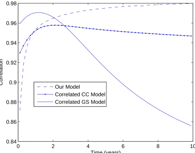
Figure 5 shows the correlation structure for correlated GS, correlated CCD and our model. The plot shows that only our model is able to generate the upward sloping correlation curve present in the data. In the short run, we see the correlation for our model is smaller than the correlated GS and CCD models. This occurs because our model is more flexible when capturing the co-movement between two futures prices, which allows us to disentangle the different sources of co-movement (i.e. the correlation and the ICE effects). Indeed, the correlated versions of GS and CCD, which don’t consider long-term ICE relationships, are forced to include some existing mid-term correlation in the short-term component of co-movement. In the long run, our model allows for a greater correlation than the other two models, which is consistent with the significance of the ICE relationship.
In the next section we show that a well-behaved empirical model can guide investors in correctly pricing financial contingent claims.
6
Application – Spread Option Valuation
Spread options are based on the difference between two commodity prices. This difference can be, for example, between the price of an input and the price of the output of a production process (processing spread). NYMEX offers tradable options on the crack spread: the heating oil/crude oil and gasoline/crude oil spread options (introduced in 1994) and the recently announced substitute spread between the WTI and the Brent crude oil. Also, many firms may face “real options” on spreads. For example, manufacturing firms possess an option of transferring the raw material to products at a certain cost, because they can choose not to produce. This option is on the spread between input and output prices and the strike price corresponds to the production cost. The spread option is of great importance for both commodity market participants and real production firms.
Since the spread is determined by the difference of two asset price, it is natural to model the spread by modeling each assetseparately. This is the main characteristic of the so-called two-price model, where the short-term correlation is the driver for most of the action in the spread (as in the correlated GS and CCD models). Up to now, nearly all researchers use the two-price model for pricing spread options (see Margrabe (1978) and Carmona and Durrleman (2003)). However,
as we see from section 4.2, the two-price model ignores the long-term co-movement component implied by ICE relationship. Thus, the two-price models might be flawed especially for the long run. Mbanefo (1997) and Dempster, Medova, and Tang (2008), among others have documented that the traditional two-price model suffers a problem of overpricing the spread option. Therefore, spread option pricing can be regarded as an out-of-sample test for our theoretical model.
At current timet, the pricing of call and put spread options,ct(T, M) and pt(T, M), with strike
K on two commodities with futures pricesF1,t(M) and F2,t(M), are specified as:
ct(T, M) = e−r f(T−t) EQt [max (F2,T(M)−F1,T(M)−K,0)] (32) pt(T, M) = e−r f(T−t) EQt [max (K−(F2,T(M)−F1,T(M)),0)] (33)
where the time to maturity for the spread options isT. To the best of our knowledge, the analytical solution for spread options is not available ifK6= 0. Thus, to price the options we use Monte Carlo simulation. In this section, we simulate the futures prices using three models – ours, the correlated CCD, and the correlated GS models. The futures price dynamics under the risk-neutral measure are specified as,
dFi,t(M)
Fi,t(M)
=Gi(M−t)dβQ, for i= 1,2 (34)
We choose two spread options: the crack spread option – spread between heating oil and the WTI crude oil, and the substitute spread option – spread between the WTI crude oil and Brent crude oil. For the crack spread, we assume crude and heating oil prices asF1,t(M) = 100 (crude oil) and
F2,t(M) = 105 (heating oil), respectively; and for Brent and WTI crude oil, we useF1,t(M) = 100
(Brent crude) and F2,t(M) = 102 (WTI crude), respectively.14
We focus on spread options of different maturities to understand the effect of the correlation structure implied by the models. We choose T = 3 month for short-maturity options and T = 5 years for long-maturity options. Also, for both, crack and substitutive spreads, we choose the same maturity on futures and options, which is the convention of the spread option specification on NYMEX. We use the estimates from the crude-heating oil and WTI-Brent oil pairs to conduct our simulations, where 2000 paths are simulated for the three models. In order to make the simulation
14
Note that generally heating oil is about 5 dollars higher than the crude oil, and WTI crude is 1.5 to 2 dollars above Brent crude.
accurate, we use anti-variate techniques in generating random variables and use the same random seed for all three models. The risk free rate rf is 0.04 in the simulation.
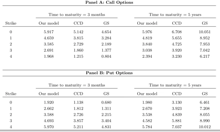
Tables 4 and 8 show the option values with different strikes for both call and put options of crack spread and substitutive spread, respectively. The tables show that both, short-term and long-term effects, are important determinants of spread option prices. The results indicate that for long-maturity options (T = 5 years), our model implies lower call and put spread option prices than the correlated GS and CCD models.15 Our finding is consistent with the evidence of Mbanefo (1997) that the two-prices models tend to overprice the spread option by ignore the equilibrium relationship, specially for long-maturity options. This is a consequence of the higher long-term correlations implied by our model. Intuitively, the ICE relationship (positive b1,2 and b2,1’s) restrict the commodity prices from large deviations from their equilibrium, and thus make the
spread of the prices relatively smaller and less volatile than models without the ICE specification. The lower term volatility of the spread traduces into lower options values.
The opposite occurs for short-maturity options (T = 3 month). The results suggest that the two-prices model may underprice short-maturity option values. The short-term correlation in the CCD and GS models is contaminated because these models are misspecified.16 Indeed, these models can not capture the term source of co-movement, therefore, they tend to accommodate long-term effects in the short-end of the correlation structure. This creates important biases in option prices.
7
Conclusions
We study the determinants of the co-movement among commodity prices in a multi-asset frame-work. We find that a long-term source of co-movement is driven by economic relations, such as, production, substitution or complementary relationships. We refer to these economic connections as inter-commodity equilibrium (ICE) relationships. Using a structural model, we show that the
15Note that CCD model has lower option prices than those in the GS model because the CCD model captures the mean-reversion of commodity prices, while GS model does not.
16Figures 5 and 9 show that the cross-commodity feedback effect in our model implies a lower short-term correlation and a larger long-term correlation than the correlated GS and CCD models.
ICE relation implies a cross-commodity feedback effect that influence the long-term joint dynamics of prices. This effect implies that the convenience yield of a certain commodity depends on the prices of other related commodities. This notion is not presented in the traditional “Theory of Storage”.
We propose a maximal affine reduced-form model for a multi-commodity setup which nests the GS and CCD models. We follow the ICE prediction and explicitly consider the interdependence of convenience yields on the spot prices of all commodities in the economy. Our model allows us to disentangle the different sources of co-movement and implies a flexible correlation structure that matches the upward sloping shape observed in the data for ICE commodities. We find that traditional commodity pricing models, such as the GS and CCD models, impose strong restrictions on the correlation structure. These models account only for a short-term source of co-movement, therefore the estimation forces this component to accommodate to match the higher long-term correlations in the data. We estimate our model for the heating oil crude oil and for the WTI -Brent crude oil pairs. Likelihood-ratio tests show that our model is significantly better than the correlated versions of the GS and CCD models, which proves the importance of modeling ICE relationships.
We use our model to price spread options because spread options largely depend on the equi-librium relationship between the two underlying commodities. The flexibility in the correlation structure implied by our model has an important effect on option prices. For long-maturity op-tions, our model predicts lower prices than those from the correlated GS and CCD models. This occurs because our model correctly accounts for an upward sloping correlation structure. The long-run relationship ties both commodity prices, reducing the volatility of the spread and yielding lower spread option values. Our results also show that the short-term correlation is lower than the one in the GS and CCD models. This imply higher prices for short-maturity spread options.
References
Ai, Chunrong, Arjun Chatrath, and Frank Song, 2006, On the comovement of commodity prices,
American Journal of Agricultural Economics 88, 574–588.
Banerjee, Anindya, Juan Dolado, John W. Galbraith, and David Hendry, 1993, Co-Integration, Error Correction, and the Econometric Analysis of Non-Stationary Data . Advanced Texts in Econometrics (Oxford University Press) 2nd edn.
Bessembinder, Hendrik, Jay F. Coughenour, Paul J. Seguin, and Margaret Monroe Smoller, 1995, Mean reversion in equilibrium asset prices: Evidence from the futures term structure, Journal of Finance 50, 361–375.
Brennan, Michael J., 1991, The price of convenience and the valuation of commodity contingent claims, in D. Lund,andB. Oksendal, ed.: Stochastic Models and Option Values (North Holland). Carmona, Ren´e, and Valdo Durrleman, 2003, Pricing and hedging spread options, SIAM Review
45, 627–685.
Casassus, Jaime, and Pierre Collin-Dufresne, 2005, Stochastic convenience yield implied from com-modity futures and interest rates, Journal of Finance 60, 2283–2332.
, and Bryan Routledge, 2008, Equilibrium commodity prices with irreversible investment and non-linear technology, Working Paper, Columbia University.
Cortazar, Gonzalo, Carlos Milla, and Felipe Severino, 2008, A multicommodity model of futures prices: Using futures prices of one commodity to estimate the stochastic process of another,
Journal of Futures Markets 28, 537–560.
Cox, John C., Jonathan E. Ingersoll Jr., and Steve A. Ross, 1985, An intertemporal general equi-librium model of asset prices, Econometrica 53, 363–384.
Dai, Qiang, and Kenneth J. Singleton, 2000, Specification analysis of affine term structure models,
Journal of Finance 55, 1943–1978.
de Boef, Suzanna, 2001, Modeling equilibrium relationships: Error correction models with strongly autoregressive data, Political Analysis 9, 78–94.
Dempster, M.A.H., Elena Medova, and Ke Tang, 2008, Long term spread option valuation and hedging, Journal of Banking and Finance 32, 2530–2540.
Duffee, Gregory R., 2002, Term premia and interest rate forecasts in affine models, Journal of Finance 57, 405–443.
Duffie, Darrell, and Rui Kan, 1996, A yield-factor model of interest rates, Mathematical Finance
6, 379–406.
Duffie, Darrell, Jun Pan, and Kenneth Singleton, 2000, Transform analysis and asset pricing for affine jump-diffusions, Econometrica 68, 1343–1376.
Dumas, Bernard, 1992, Dynamic equilibrium and the real exchange rate in a spatially separated world, Review of Financial Studies 5, 153–180.
Durbin, James, and Siem Jan Koopman, 2001, Time Series Analysis by State Space Methods (Ox-ford University Press).
Energy Information Administration, 2002, Manufacturing energy consumption survey, U.S. De-partment of Energy.
Engle, Robert F., and Clive W.J. Granger, 1987, Co-integration and error correction: Representa-tion, estimaRepresenta-tion, and testing, Econometrica 55, 251–276.
Geman, Helyette, and Vu-Nhat Nguyen, 2005, Soybean inventory and forward curve dynamics,
Management Science 51, 1076–1091.
Gibson, Rajna, and Eduardo S. Schwartz, 1990, Stochastic convenience yield and the pricing of oil contingent claims, Journal of Finance 45, 959–976.
Girma, Paul B., and Albert S. Paulson, 1999, Risk arbitrage opportunities in petroleum futures spreads,Journal of Futures Markets 19, 931–955.
Hamilton, James D., 1994,Time Series Analysis (Princeton University Press).
Harvey, Andrew C., 1991,Forecasting, Structural Time Series Models and the Kalman Filter (Cam-bridge University Press).
Higham, Nicholas J., and Hyun-Min Kim, 2001, Solving a quadratic matrix equation by newton’s method with exact line searches,SIAM Journal on Matrix Analysis and Applications23, 303–316. Kaldor, Nicholas, 1939, Speculation and economic stability,Review of Economic Studies 7, 1–27. Keynes, John M., 1923, Some aspects of commodity markets, Manchester Guardian Commercial:
European Reconstruction Series.
Kogan, Leonid, Dmitry Livdan, and Amir Yaron, 2008, Oil futures prices in a production economy with investment constraints, forthcoming,Journal of Finance.
Malliaris, A. G., and Jorge L. Urrutia, 1996, Linkages between agricultural commodity futures contracts,Journal of Futures Markets 16, 595–609.
Margrabe, William, 1978, The value of an option to exchange one asset for another, Journal of Finance 33, 177–186.
Mbanefo, Art, 1997, Co-movement term structure and the valuation of energy spread options, in Michael A. H. Dempster,andStanley R. Pliska, ed.: Mathematics of Derivative SecuritiesNo. 15 in Publications of the Newton Institute . pp. 88–102 (Cambridge University Press).
Paschke, Raphael, and Marcel Prokopczuk, 2007, Integrating multiple commodities in a model of stochastic price dynamics, Working Paper University of Mannheim.
Pindyck, Robert S., 2001, The dynamics of commodity spot and futures markets: A primer.,Energy Journal 22, p1 –.
, and Julio J. Rotemberg, 1990, The excess co-movement of commodity prices, Economic Journal 100, 1173–1189.
Richard, Scott F., and M. Sundaresan, 1981, A continuous time equilibrium model of forward prices and futures prices in a multigood economy, Journal of Financial Economics 9, 347–371.
Richter, Martin C., and Carsten Sorensen, 2002, Stochastic volatility and seasonality in commodity futures and options: The case of soybeans, Working Paper, Copenhagen Business School.
Routledge, Bryan R., Duane J. Seppi, and Chester S. Spatt, 2000, Equilibrium forward curves for commodities, Journal of Finance 55, 1297–1338.
, 2001, The spark spread: An equilibrium model of cross-commodity price relationships in electricity, Working Paper, Carnegie Mellon University.
Schwartz, Eduardo S., 1997, The stochastic behavior of commodity prices: Implications for valua-tion and hedging, Journal of Finance 52, 923–973.
Smith, H. Allison, Rajesh K. Singh, and Danny C. Sorensen, 1995, Formulation and solution of the non-linear, damped eigenvalue problem for skeletal systems,International Journal for Numerical Methods in Engineering 38, 3071–3085.
Telser, Lester G., 1958, Futures trading and the storage of cotton and wheat, Journal of Political Economy 66, 233–255.
Trolle, Anders B., and Eduardo S. Schwartz, 2009, Unspanned stochastic volatility and the pricing of commodity derivatives, forthcoming, Review of Financial Studies.
Working, Holbrook, 1948, Theory of the inverse carrying charge in futures markets, Journal of Farm Economics 30, 1–28.
Appendix
A
Derivation of the Economic Model of Production Relationship
First, note that we can extract the convenience yieldδj for each commodity j using the pricing kernel (ξ) and the price of the commodity (Sj):
E[d(ξ Sj) +ξ δjSjdt] = 0 (A1) which implies that
E dχ j χj =−δjdt (A2)
with χj =ξ Sj. The interpretation for this result is that the convenience yield corresponds to the interest rate in a world that uses the commodity as the numeraire (see Richard and Sundaresan 1981, and Casassus, Collin-Dufresne, and Routledge 2008).
Let us denote by J(K, Q1, Q2) = sup{CK,u,C2,u,q1,u} ∈ AEt
R∞ t e −θ(u−t)U(C K,u, C2,u)du the “current” value function associated with the representative agent’s problem. Note that given the set-up, the value functionJ(·) is not a function of time.
The solution of the our problem is determined by the following Hamilton-Jacobi-Bellman (HJB) equation: sup
{CK,C2,q1} ∈ A
{U(CK, C2) +DJ−θJ}= 0 (A3)
whereDis the Itˆo operator
DJ = (α K−CK) ∂J ∂K −q1 ∂J ∂Q1 + (γlog(q1)Q2−C2) ∂J ∂Q2 +1 2σ 2 KK2 ∂2J ∂K2 (A4) with ∂J ∂K, ∂J ∂Q1 and ∂J
∂Q2 representing the marginal value of an additional unit of numeraire good, crude oil and heating oil, respectively. ∂K∂2J2 is the second derivative with respect toK.
The first-order conditions with respect to consumption of capital, consumption of heating oil and demand for crude oil areUCK=
∂J ∂K,UC2 = ∂J ∂Q2 and γ Q2 q1 ∂J ∂Q2 = ∂J
∂Q1, respectively. Given our logarithmic utility func-tion, these conditions imply that the optimal consumptions areCK =φ ∂K∂J
−1 andC2= (1−φ) ∂J ∂Q2 −1 . After replacing these controls in the HJB equation we obtain an ordinary differential equation with a closed-form solution that is linear in log(K), log(Q1) and log(Q2).
We note that the pricing kernel isξt∝e−θ tUCK,t(CK,t, C2,t) and define commodity prices as the marginal prices that solveJ(K, Q1, Q2) =J(K+S1, Q1−, Q2) =J(K+S2, Q1, Q2−) when→0. These imply
thatSj= ∂K∂J
−1 ∂J
∂Qj forj∈ {1,2}. Finally, using the envelope condition above, we obtain the result that commodity j pricing kernel isχj,t ∝ e−θ t ∂J
(Kt,Q1,t,Q2,t)
∂Qj . We apply Itˆo’s to this expression to obtain the convenience yield of commodityj.
B
Substitute and Complementary Relationships
B.1 The Economic Model for a Substitute Relationship
Consider now a similar economy to the production case in Section 3, but with two substitute commodities, say, West Texas Intermediate (WTI) crude oil from the North Sea (Q1) and Brent crude oil (Q2). There
is also a production technology in the capital sector (K) that uses both types of crude oils to produce the consumption good. The representative agent in the economy maximizes the expected log utility with respect to the consumption of capital (CK), the demand of WTI crude oil (q1) and the demand of Brent crude
oil (q2): sup {CK,t,q1,t,q2,t} ∈ A E0 Z ∞ 0 e−θ tlog (CK,t)dt (B1) whereAis a set of admissible strategies. First, consider a simple case where the capital and crude oil stocks evolve in the following way:
dK = (α(log(q1) + log(q2))K−CK)dt+σKKdWK (B2)
dQ1 = −q1dt+σ1Q1dW1 (B3)
dQ2 = −q2dt+σ2Q2dW2 (B4)
The uncertainty is captured by the independent Brownian motions Wi for i ∈ {K,1,2}. The stochastic crude oil stocks capture the fact that available barrels of oil are affected by some exogenous factors. As we will note later, this type of uncertainty generates the very appealing feature that the WTI and Brent crude oil prices are less than perfectly correlated.
At this point, given the simplicity of the economy, the two commodities Q1 andQ2 are not substitutes.
The crude oil demandsq1andq2depend only on their own stock level. Whether the WTI crude oil is cheaper
or more expensive than the Brent crude oil does not affect the demand for Brent oil.
A simple way of making these two commodities substitute is by allowing some interaction between the two crude oil stocks. For example, if the agents can move some units from the Brent stock to the WTI stock and vice-versa, then the two commodities will have some degree of substitutability. There are multiple ways of doing this, but only few of them have closed-form solutions. It is important to have analytical expressions in order to understand the economics behind the results.
The case with optimal adjustment from Brent to WTI crude oil and vice-versa at an infinite rate and at no cost can easily be solved, but the model is unrealistic. Without any friction both crude oil prices will be identical. If we consider some degree of irreversibility by including proportional adjustment costs, the problem becomes similar to that of the shipping model of Dumas (1992) which needs to be solved numerically.17 Including fixed costs as in Casassus, Collin-Dufresne, and Routledge (2008) involves an even
more complex solution. If there is a finite upper bound for the rate of adjustment from one stock to the other, the problem has the same flavor as in the bounded investment rate model of Kogan, Livdan, and Yaron (2008). Because of the extra state variable, to the best of our knowledge, there is no closed form solution to this problem, either.
A common characteristic of the endogenous decisions in the three equilibrium models mentioned above is that the optimal adjustment occurs when the level of the target stock is relatively lower than the level of the source stock. We propose an exogenously defined adjustment strategy that captures this feature and allows for closed-form solutions. The strategy involves transporting a time-varying fraction of Brent oil stocks to the WTI sector when the Brent stocks are greater than the WTI stocks, and vice-versa. Doing this at a finite rate captures the irreversibility characteristic embedded in the endogenous decisions of Dumas (1992), Casassus, Collin-Dufresne, and Routledge (2008) and Kogan, Livdan, and Yaron (2008). The modified processes are:
dQ1 = (ω Q1−q1)dt+σ1Q1dW1 (B5) dQ2 = (−ω Q2−q2)dt+σ2Q2dW2 (B6) dω = κ log Q 2 Q1 −ω dt (B7)
The adjustment rateω can take both signs. It moves continuously towards a time-varying long-term mean that depends on the stocksQ1andQ2. If there is more Brent oil than WTI oil in the economy (i.e. Q2> Q1),
17
Actually, the problem here is more complex, since we have three state variables instead of the two state variables representing the two countries in Dumas (1992).
the rate ω moves towards a positive value until the stocks are balanced. The positive parameter κis the speed of adjustment from one oil stock to the other and captures the degree of substitutability between the two commodities. The higher the κ the better substitutes are the commodities, because the adjustment occurs at a higher speed. It also captures the persistence of the adjustment rate, and thus the degree of irreversibility in the adjustment decision. A low κimplies greater irreversibility because it will take longer to balance the stocks.
Let us denote byJ(K, Q1, Q2, ω) = sup{CK,u,q1,u,q2,u} ∈ AEt
R∞
t e
−θ(u−t)U(CK,u)du
the “current” value function for the representative agent’s problem in the substitute relationship example.
The solution to our problem is determined by the following Hamilton-Jacobi-Bellman (HJB) equation: sup
{CK,q1,q2} ∈ A
{U(CK) +DJ−θJ}= 0 (B8)
where D is the standard Itˆo operator associated to this economy. The first-order conditions with respect to consumption of capital and demands for the two types of crude oil are CK = ∂K∂J
−1 , α Kq 1 ∂J ∂K = ∂J ∂Q1 and α Kq 2 ∂J ∂K = ∂J
∂Q2, respectively. After replacing these controls in the HJB equation we obtain an ordinary differential equation with a closed-form solution that is linear in log(K), log(Q1), log(Q2) andω.
The representative agent problem that maximizes equation (B1) subject to equations (B2) and (B5)-(B7) has an affine solution similar to the one in the production relationship example. The representative agent optimally consumes a constant fraction of capital (CK =θ K) and demands a constant rate of WTI and Brent crude oils (q1 =θ Q1 andq2=θ Q2). Note that as before, the instantaneous crude oil demands
are a function only of their own crude oil stocks, but now both crude oil stocks are related because of the adjustment rateω. This implies that future Brent oil demands will be affected by the current WTI stock level.
In a similar way to the production relationship, the equilibrium crude oil prices are very simple:18
S1= α θ K Q1 and S2= α θ K Q2 (B9) The prices have the same structure, because the problem is symmetric for both commodities.19 The equi-librium convenience yields are:
δ1=ω−σ12 and δ2=−ω−σ22 (B10)
The convenience yields are directly related to the adjustment rate ω. The WTI oil convenience yield is increasing inω, because a highω implies more expected WTI oil stocks in the next period.20 This expected
increase in stocks decreases expected prices, thus generating a positive convenience yield (after risk premium adjustments). The WTI oil convenience yield is time varying and has the same dynamics as the adjustment rate. If we also consider that equation (B9) implies that Q2Q
1 = S1
S2, then the dynamics ofδ1 is:
dδ1=κ log S 1 S2 −δ1 dt (B11)
A higher differential between S1 andS2 implies that the convenience yieldδ1 is more likely to increase in
the near future. In this particular case, the convenience yields are conditionally deterministic, because the exogenous adjustment strategy was assumed to have this characteristic. Equation (B12) shows that the convenience yield of WTI oil depends on the price of Brent crude oil,
δ1,t=δ1,t0e −κ(t−t0)+ Z t t0 κ e−κ(t−u)log S1,u S2,u du (B12) 18
Again, see Appendix A for more details on the solution of the model. 19Note that becauseQ
1 andQ2 are driven by independent Brownian motions, the price of the commodities are only partly correlated. This correlation emerges because they share the common factorK.
20