The partition of unity parallel finite element algorithm
Haibiao Zheng·Lina Song·Yanren Hou· Yuhong Zhang
Received: 19 November 2013 / Accepted: 22 October 2014 / Published online: 7 November 2014
© Springer Science+Business Media New York 2014
Abstract This paper presents a partition of unity parallel finite element algorithm. This algorithm localizes the global residual problem of two grid method into some parallel local sub-problems, and use a simple partition of unity to assemble all the local solutions together. An oversampling technique is used and analyzed to decrease the undesirable effect of the artificial homogeneous Dirichlet boudary condition of local sub-problems. The analysis shows the error of this algorithm decays expo-nentially with respect to the oversampling parameter. Specially, on a regular coarse triangulationτH with mesh size H, an oversampling of diameter Hlog(1/H ) is
sufficient to preserve the optimal convergence order. Numerical results verify the theoretical analysis.
Keywords Two-grid methods·Parallel·Partition of unity·Oversampling Mathematics Subject Classification 65N30·65N50·65N55.
Communicated by: Jinchao Xu H. Zheng ()
Department of Mathematics, East China Normal University, Shanghai, China e-mail: [email protected]
L. Song
College of Mathematics, Qingdao University, Qingdao, China e-mail: [email protected]
Y. Hou·Y. Zhang
School of Mathematics and Statistics, Xi’an Jiaotong University, Xi’an, China e-mail: [email protected]
Y. Zhang
1 Introduction
In last decades, local and parallel finite element computations have become very attractive. Based on two-grid discretization, Xu and Zhou [1], Bank and Holst [2, 3] presented some local and parallel finite element algorithms for elliptic boundary value problems. Their main idea is high frequency components of solution can be captured locally on a fine grid, while low frequency components could be approx-imated on a relatively coarse grid. The advantage of such algorithms lies in less communication between blocks during locally computing high frequency compo-nents. Due to above advantage, theses algorithms were widely extended to other model problems, such as, Stokes equations [4], Navier-Stokes equations [5–7], and the convection diffusion problems [8]. Moreover, the partition of unity method (PUM) [9,10] plays an important role during the development of local and parallel algorithms. Holst [11,12] combined the PUM with the parallel adaptive algorithm to improve the local and parallel algorithms, and constructed the parallel partition of unity method (PPUM). Wang, Huang and Li [13] also developed two-grid parti-tion of unity method for second order elliptic problems. Huang and Xu [14] applied the partition of unity finite element method for elliptic problems with highly oscil-lating coefficients. Bacuta and his co-authors [15] researched the partition of unity method on nonmatching grids. Recently, Zheng and co-authors [16,17] developed the local and parallel finite element algorithms based on the partition of unity for the incompressible flows.
In this paper, based on the partition of unity method, we design a new local and parallel finite element algorithm for the following elliptic boundary value problem defined on a convex polyhedral domain⊂Rd, d=2,3:
−u+b· ∇u=f in ,
u=0 on ∂. (1.1)
The partition of unity parallel finite element algorithm is constructed as follows. Step 1. Solve (1.1) on a coarse gridτH using the standard finite element method.
Step 2. Decompose the whole domaininto a series of local sub-domains{i},
which are associated with nodal basis functions{φi}based onτH.
Step 3. Solve local residual problems with homogeneous Dirichlet boundary con-ditions on fine grids of{i}, then locally correct the standard finite element
approximation in Step 1.
Step 4. Assemble all the local solutions together by the partition of unity{φi}to get
a global continuous finite element solution.
We have to illustrate the choice of local sub-domains{i}in Step 2. Naturally{i}
should be the impact domain{ωi}of nodal basis functions{φi}, namely, supp{φi}∩.
However, if local sub-domains{ωi}are not large enough, then the artificial
homo-geneous Dirichlet boundary condition of local problems would decrease the global accuracy. Therefore, oversampling of multi-layer {ωi,k}are introduced to enlarge
{ωi}. Obviously, it is important to choose the oversampling parameterkto
k ≈ O(log(1/H ))is sufficient to preserve the optimal convergence order for the above algorithm.
The main differences between our algorithm with existing PPUM lie in two aspects. One is the way to choose partition of unity functions. The classical PPUM constructs the partition of unity functions according to the given domain decomposi-tion. However, our algorithm uses the nodal basis functions on the coarse grid as the partition of unity functions, and derives domain decomposition by the basis functions. Obviously, our algorithm is more natural and simpler to define partition of unity func-tions and decompose the whole domain. Another difference is the way to estimate the global error. The estimations of classical PPUM usually rely on the large overlap assumption and the number of local sub-domains. However, without any assump-tion, we use an oversampling technique to decide an appropriate size of sub-domains to obtain the optimal error order. Moreover, our estimations are independent of the number of local sub-domains. Such oversampling technique have be applied in many other fields, such as multiscale methods [18–20] and adaptive postprocess [21,22].
The outline of the paper is organized as follows. Section2introduces some prelim-inaries. The partition of unity parallel finite element algorithm and its oversampling technique are discussed and analyzed in Sections3. In Sections4, the implementa-tion details and some numerical simulaimplementa-tions are presented to illustrate the efficiency of our algorithm. A short conclusion will be given in final Sections5.
2 Preliminaries
Firstly, for a convex polyhedral domain ⊂ Rd, we use standard notations for Sobolev spaces Ws,r() and their associated norms, see, e.g., [23] and [24]. In particular, forr = 2, we denote byHs() = Ws,2(), equipped with the norm
· s,= · s,2,, and byV =H01()= {v∈H1(): v|∂=0}the subspace of
H1()with zero trace, equipped with the usual norm∇ ·0,or its equivalent norm
· 1,due to the Poincare’s inequality. In the following, the symbol(·,·)denotes
the inner product inL2()or in its vector value version. The spaceH−1()is also used to denote the dual ofH01(), we use<·,·>to denote the dual inner between H−1()andH01().
For sub-domains D ⊂ G ⊂ , the notation D ⊂⊂ G means that dist(∂D\∂, ∂G\∂) >0.
LetτH be a triangulation of with mesh parameter H = max T∈τH
diam(T ). The classical (conforming)P1finite element space is given by
VH := {v∈C0()¯ | ∀T ∈τH, v|Tis a polynomial of total degree≤1},
here,C0()¯ is a space of continuous functions on.¯
Meanwhile, recall the local approximation and stability properties of the nodal interpolation operatorSH : V → VH respect to the meshτH:∀v ∈ V , ∀T ∈ τH,
there exists a general constantCsuch that
whereCdepends on the shape regularity parameterρof the meshτH but not onH.
2.1 The standard Galerkin method and two-grid method
The standard variational formulation of Eq.1.1is given by: for anyf ∈ H−1(), findu∈V such that
B(u, v)=< f, v > ∀v∈V . (2.2) where the bilinear formB(·,·)is defined by
B(u, v):=a(u, v)+(b· ∇u, v),
and a(u, v) := (∇u,∇v). A sufficient and necessary condition for the well-posedness of Eq.2.2is w1,≤Csup φ∈V B(w, φ) φ1, , sup φ∈V B(φ, w) φ1, ∀ w∈V ,
The variational problem (2.2) has a unique solution(see e.g., [25]). Hereafter,C is a generic positive constant that may stand for difference values at different places.
It is well-known that the standard finite element solution of Eq.2.2uH ∈VH0 :=
VH∩V satisfies
B(uH, v)=< f, v > ∀v∈VH0, (2.3)
and the error estimate
u−uH0,+Hu−uH1,≤CH2u2, (2.4)
holds providedu∈H2().
For the two-grid discretization of problem (2.2), we shall need another triangula-tionτhofwith mesh parameterh, and related piecewise linear finite element space
Vh. For simplicity, we always assume thatτhis a refinement ofτH. Hence, we shall
callτH a coarse mesh, andτha fine mesh, and haveVH ⊂Vh.
The standard two-grid method of Eq.2.2is to finduh=uH+ehwithuh ∈Vh0=
Vh∩V , uH ∈VH0, eh ∈Vh0such that
B(uH, v)=< f, v > ∀v∈VH0, (2.5)
a(eh, v)=< f, v >−B(uH, v) ∀v ∈Vh0. (2.6)
And the optimal error estimate (see Xu [27])
u−uh1,≤C(h+H2)u2, (2.7)
holds.
3 The partition of unity parallel finite element algorithm(PUPM)
In this section, we use localization and oversampling techniques to improve the standard two-grid method, and propose a partition of unity parallel finite element algorithm.
3.1 The partition of unity, oversampling and algorithm
We firstly introduce some notations. Given a regular triangulationτH of, for each
vertexxi∈τH, i=1,2,· · ·, N,letωi⊂denote the union of triangles sharingxi,
and denoteφiby the linear, continuous lagrangian basis function such thatφi(xj)=
δi,j. Then, the local computational domain with respect toxi for partition of unity
without oversampling isωi=suppφi∩.
For simplicity, letk∈N, denote nodal patches ofkth orderωi,kaboutxi∈τH by
ωi,1:=ωi=suppφi∩,
ωi,k:=
xj∈ωi,k−1
ωj,1, k=2,3,· · ·,
and corresponding local finite element spaces
VhH(ωi,k):= {v∈Vh|v|\ωi,k =0}.
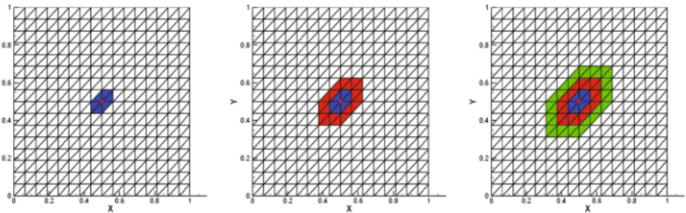
The oversampling parameterkplays an important role in our algorithm. Figure1will help us to undersand the local domain with oversampling. Note that,
N
i=1
φi≡1, and
∀i, k, suppφi⊂ωi,k,we could call{φi}N1 is a partition of unity subordinate to the
local domains{ωi,k}N1.
In next subsections, we will analyze the choice ofkto guarantee both efficiency and accuracy of the algorithm.
Now we are in the position to present the algorithm.
ALGORITHM PUPM:
Step 1. Find a global coarse grid solutionuH ∈VH0 such that
B(uH, v)=< f, v > ∀v∈VH0. (3.1)
Step 2. Correct the residual on a fine grid in each overlapping sub-domainωi,km
(here,m∈ Nandm≥ 1 is given), namely, for eachi =1,· · ·, N, solve
Fig. 1 The local computational domain. Left, a local domain without oversamplingωi,1=bule region;
middle, one layer of oversamplingωi,2=bule and red regions; right, two layers of oversampling denoted
ehi,km∈Vh,i,kmH,0 :=VhH(ωi,km)∩V by
a(ehi,km, v)=< f, v >−B(uH, v) ∀v∈Vh,i,kmH,0 . (3.2)
Step 3. Update:ui=uH+ehi,kminωi,km.
Step 4. Construct the finite element solutionu˜h =
N
i=1
φiui.
The main difference between this algorithm and standard two-grid method lies in Step 2, the correction step. We localize the global residual problem (2.6) into some local subproblems (3.2) with homogeneous Dirichlet boundary conditions. Moreover, these subproblems are independent and can be solved parallel. In next subsections, our analysis will show local domains of diameterHlog(1/H )are sufficient to pre-serve the optimal convergence order. In the end, we use the partition of unity to assemble all the local solutions together in Step 4.
3.2 Truncation error analysis for oversampling We introduce a useful cut-off function.
Definition 1 Forxi ∈ τH andd <D∈ N, letηd,i D : → [0,1]be a continuous,
linear and weakly differentiable function such that
ηd,i D|ωi,d =1, ηd,i D|\ωi,D =0, ∀T ∈τH, ||ηid,D||L∞(T )≤C∞, (3.3) ∀T ∈τH, ||∇ηid,D||L∞(T )≤CG 1 (D−d)H, (3.4) where constantsC∞andCGonly depend on the regularity parameterρof the mesh
τH but not onH.
Theorem 3.1 (Truncation error) Let ei,kmh be the solution of the residual problem (3.2). The estimate
||ei,kmh ||21,ωi,m ≤θ
k−1||
ehi,km||21,ωi,km. (3.5)
holds, whereθ := m2HC(H2+C(H+1)+1) and constantConly depends on on the regularity
parameterρ.
Proof For allxi ∈ τH, 1 ≤ j, m, k ∈ N, letθj := η(ji −1)m,j m, 2 ≤ j ≤ k,as
inDefinition 1. It is obvious thatSH(θj2ehi,km) ∈ V H,0
a(ehi,km, vH)=0 for any functionvH inVh,i,kmH,0 ∩VH0 gives
||ehi,km||21,ωi,(j−1)m ≤ ||θje
h
i,km||21,ωi,j m ≤ C||∇(θjei,kmh )||20,ωi,j m
= Caehi,km, θj2ei,kmh +C∇θjehi,km,∇θjehi,km
= Caehi,km, θj2ei,kmh −SH
θj2ei,kmh +C∇θjei,kmh ,∇θjei,kmh
. For the first term, using Cauchy-Schwarz inequality and (2.1) gives
a ehi,km, θj2ei,kmh −SH(θ 2 jei,kmh ) ≤C||∇ehi,km||0,ωi,j m||∇ ×θj2ehi,km−SH(θ 2 jehi,km) ||0,ωi,j m ≤ C||∇ei,kmh ||0,ωi,j m × ⎛ ⎝ T⊂ ¯ωi,j m ||∇θj2ehi,km−SH θj2ei,kmh ||2L2(T ) ⎞ ⎠ 1/2 ≤ C||∇ei,kmh ||0,ωi,j mH × ⎛ ⎝ T⊂ ¯ωi,j m ||∇2 (θj2ehi,km)||2L2(T ) ⎞ ⎠ 1/2 .
Sinceθj andehi,kmare linear,∇2θj = ∇2ehi,km =0 in every elementT ∈ τH, T ⊂
ωi,j m. Moreover, using the property of cut-off functions in Eq.3.4and definition of
θj yields || ∇ ehi,km||0,ωi,j mH ⎛ ⎝ T⊂ ¯ωi,j m ||∇2 (θj2ehi,km)||2L2(T ) ⎞ ⎠ 1/2 = ||∇ehi,km||0,ωi,j mH ⎛ ⎝ T⊂ ¯ωi,j m ||(∇θj)2ei,kmh +2θj∇θj∇ehi,km|| 2 L2(T ) ⎞ ⎠ 1/2 ≤ C||∇ei,kmh ||0,ωi,j mH × ⎛ ⎝ T⊂ ¯ωi,j m (||∇θj||4L∞(T )||e h i,km|| 2 L2(T )+ ||∇θj||2L∞(T )||∇e h i,km|| 2 L2(T ) ⎞ ⎠ 1/2
≤ C||∇ei,kmh ||0,ωi,j m\ωi,(j−1)m ×
1 m2H||e
h
i,km||0,ωi,j m\ωi,(j−1)m+
1 m||∇e
h
i,km||0,ωi,j m\ωi,(j−1)m ≤ C 1 m2H||e h i,km|| 2 1,ωi,j m\ωi,(j−1)m
where,mH ≤1 holds usually. For the second term,
(∇θjehi,km,∇θjehi,km) ≤ C 1 m2H2||e h i,km|| 2 0,ωi,j m\ωi,(j−1)m ≤ C 1 m2H2||e h i,km|| 2 1,ωi,j m\ωi,(j−1)m .
Combining all the above inequalities and letC1=C 1 m2H + 1 m2H2 , we have ||ehi,km||21,ω i,(j−1)m ≤ C1||e h
i,km||21,ωi,j m\ωi,(j−1)m = C1||ehi,km||21,ωi,j m−C1||e h i,km||21,ωi,(j−1)m. Therefore, settingθ= C1 1+C1 gives ||ei,kmh ||21,ω i,(j−1)m ≤ θ||e h i,km|| 2 1,ωi,j m.
It’s easy to have
||ei,kmh ||21,ωi,m ≤ θ||ehi,km||21,ωi,2m
≤ · · ·
≤ θk−1||ehi,km||21,ωi,km.
The proof is completed.
Remark 1 Note thatθ <1 always stands. It is because that the parametersm, H and hare given, when we discuss the property of the local residual solutionei,kmh . 3.3 Error analysis
Before estimate the error ofALGORITHM PUPM, we introduce the following lemma to show the property of partition of unity .
Lemma 3.2 Suppose{φi}Ni=1be the partition of unity based onτH. Then, there exists
a constantCindependent ofN, such that
N i=1 φiv 2 1, ≤C N i=1 φiv21,ωi ∀v∈H 1 0(). (3.6)
Proof Firstly,{xi}Ni=1are all nodes of coarse triangulationτH, which are related with
the continuous, lagrangian basis function{φi}Ni=1. For any nodexi, introduce
Wi= {xj : xj ∈suppφi}
to denote all the nodes sharing same element withxi on the triangulationτH. Then
define
Wmax:= max i=1,···,N#Wi,
which is independent ofN, due to the regularity of triangulationτH. Moreover, for
eachi, j =1,· · ·, N, ifxj ∈/ Wi, there hold(∇(φiv),∇(φjv)) =0,(φiv, φjv) =
0,∀v∈H01(),therefore, N i=1 φiv 2 1, = N i=1 N j=1 (∇(φiv),∇(φjv))+(φiv, φjv) = N i=1 xj∈Wi (∇(φiv),∇(φjv))+(φiv, φjv) ≤ N i=1 xj∈Wi (||∇(φiv)||0,||∇(φjv)||0,+ ||φiv||0,||φjv||0,) ≤ 1 2 N i=1 xj∈Wi ||∇(φiv)||20,+||∇(φjv)||20,+||φiv||20,+ ||φjv||20, ≤ Wmax N i=1 ||φiv||21,ωi.
The proof is completed.
Theorem 3.3 Assume the triangulationsτHandτhsatisfyVH ⊂Vh. Letuanduhbe
the solutions of model problem(1.1)and standard two-grid method(2.5–2.6), respec-tively. Ifu˜his the solution ofALGORITHM PUPMwith the oversampling parameter k≈O(logH1), then the following estimates
||uh− ˜uh||1,≤CH2||u||2,, (3.7)
||u− ˜uh||0,≤C(h+H2)||u||2,, (3.8)
hold.
Proof Since {φi}N1 are continuous, Lagrangian basis functions associated with a
partition of unity onτH, there holds N i=1 φi =1, and therefore,uh =uH+ N i=1 φieh . Using Lemma 3.2 yields
||uh− ˜uh||21, = || N i=1 φieh− N i=1 φiehi,km||21, ≤ C N i=1 ||φieh||21,ωi+ N i=1 ||φiehi,km||21,ωi .
Ifωi,km = , theneh = ei,kmh . Thus, Theorem 3.2 also holds foreh . By Theorem 3.1, we have N i=1 ||φieh||21,ωi+ N i=1 ||φiehi,km|| 2 1,ωi ≤ C 1 H2 N i=1 ||eh||21,ω i+ ||e h i,km|| 2 1,ωi ≤ C 1 H2 N i=1
||eh||21,ωi,m+ ||ei,kmh ||21,ωi,m
≤ C 1 H2θ k−1 N i=1 ||eh||21,ωi,km+ ||e h i,km|| 2 1,ωi,km ≤ CCov(km)d 1 H2θ k−1|| u−uH||21, +C 1 H2θ k−1 N i=1 ||u−uH||21,ωi,km ≤ CCov(km)d 1 H2θ k−1|| u−uH||21, ≤ CCov(km)dθk−1||u||22, ≤ CH4||u||22,.
Here we use the fact that for each elementTj ⊂ τH, there exists at least one local
domainωi,kmsuch thatTj ⊂ωi,km, and the number of such local domains can be
lim-ited byCov(km)d. Moreover, let the oversampling parameterk≈O(logH1)together
withθ= C(H+1)
m2H2+C(H+1) <1, we haveθk−
1≈H4.
Using Eqs. 2.5,2.6and3.2together with above analysis yields
||eh||1, ≤ C||u−uH||1,,
||ehi,km||1,ωi,km ≤ C||u−uH||1,ωi,km.
Thus, whenk≈O(logH1), we have
||uh− ˜uh||21, ≤ CH2||u||2,.
Finally, using the triangle inequality and Eq. 2.7gives
||u− ˜uh||1, ≤ ||u−uh||1,+ ||uh− ˜uh||1,≤C
h+H2
||u||2,.
The proof is finished.
Table 1 H1−error of PUPM without oversampling
H h km u− ˜uh1, Order
1/8 1/64 1 2.61737×10⁻¹
1/16 1/256 1 1.02085×10⁻¹ 0.67917
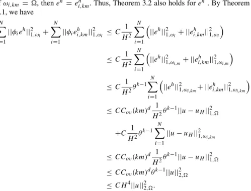
Table 2 H1−error of PUPM with oversamplingk≈2 log(1/H ),m=1 H h km u− ˜uh 1, Order 1/8 1/64 1 2.61737×10⁻¹ 1/16 1/256 2 5.70154×10⁻² 1.09935 1/24 1/576 3 2.47786×10⁻² 1.02764 4 Numerical experiments
To verify the analysis results, we consider the following simple 2-D numerical exam-ple. The algorithm in all experiments is implemented by the public finite element software Freefem++ [28]. All simulations are performed on a Dawning parallel clus-ter composed of 32 nodes, each with eight-core 2.0 GHz CPU, 2 GB×8 DRAM, and connected together by 20Gbps InfiniBand. The message-passing is supported by MPICH.
4.1 Example 1
Consider the unit square domain = [0,1] × [0,1]and take b = (1.0,1.0)T, the true solution
u(x, y)=100(x2−2x3+x4)(y−3y2+2y3). Then we can getf (x, y)in Eq.1.1.
According to Theorem 3.3, settingh = H2 and oversampling parameter k ≈ 2 log(1/H )gives
u− ˜uh1,∼O(H2)∼O(h). (4.1)
To show such convergence rate of the error, we introduce a notation ‘Order’ defined as follows. Supposee1=u− ˜uh1ande2=u− ˜uh2, then
Order:= | loge11, e21,| |logh1 h2| , (4.2)
whereh1andh2are fine mesh parameters. Then, ‘Order’ should be around 1.0 due
to Eq.4.1. Next we present numerical results to verify above theoretical results. Consider uniform coarse meshes of sizeH = 1/8, 1/16, 1/24, respectively. Their corresponding oversampling parameters arek = 1,2,3. In Tables1,2and 3, some numerical results for PUPM without and with oversampling are presented,
Table 3 H1−error of PUPM with oversamplingk≈2 log(1/H ),m=2
H h km u− ˜uh1, Order
1/8 1/64 2 1.45527×10⁻¹
1/16 1/256 4 3.62215×10⁻² 1.00318
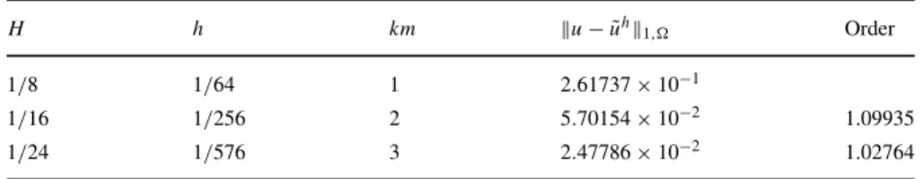
1 1.5 2 2.5 3 3.5 4 4.5 5 5.5 6 −2 −1.5 −1 −0.5 k log(|| e|| 1 ) H=1/16 H=1/24
Fig. 2 The errors decay exponentially with respect to the oversampling parameterk
respectively. Comparing ‘Order’ in Tables 2, 3 with that in Table 1, it shows that PUPM with appropriate oversampling obtains a better order of convergence than PUPM without oversampling. Moreover, comparingu− ˜uh0, in Table 2
with Table1, it presents oversampling strategy improves the accuracy of PUPM. Therefore,k≈O(log(1/H ))is sufficient to preserve the optimal convergence order. In addition, we remark the practical choice of the parameterm. Theorem 3.3, addresses for any givenm,θ <1. From Tables2and3, we know that form=1 or m=2, the results always support our theoretical analysis.
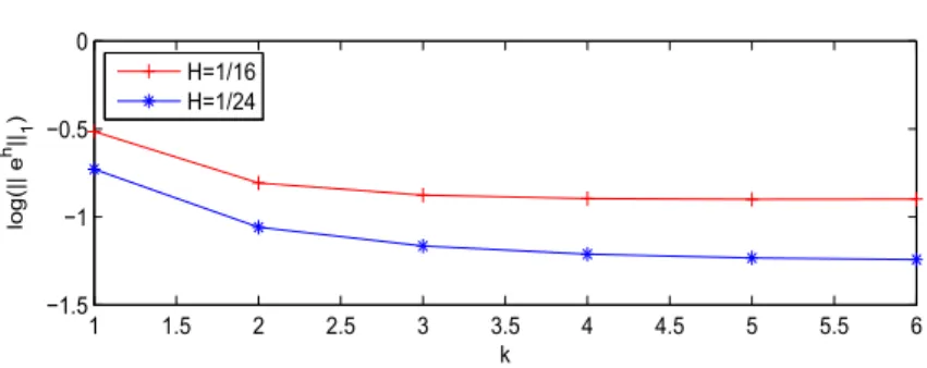
Fix m = 1 and h = H2, we present the error e := u− ˜uh of PUPM with different oversampling parameterk =1,2,3,4,5,6 in Fig.2. It shows that in both casesH =1/16 and 1/24, the error log(||e||1)decreases almost linearly respect tok,
exceptk =1. This means that the error of PUPM decays exponentially with respect to the oversampling parameterk.
4.2 Example 2
For the second example, setting b = (2x −ey,3ycos(π x)), f = 70 log((x +
0.1)(sin(πy)+1)), and = [0,1] × [0,1], we consider Eq.1.1 by zero homo-geneous boundary condition, without a true solution. According to Theorems 3.3, settingh=H2andk≈2 log(1/H )yields
||uh− ˜uh||1,∼O(H2)∼O(h).
We redefinee1 =uh1− ˜uh1ande2 =uh2− ˜uh2in the expression of ‘Order’ (4.2).
Thus, ‘Order’ should also be around 1.0.
We still consider the coarse meshes of sizeH = 1/8, 1/16, 1/24 respectively. The corresponding computational results are shown in Table4.
Table 4 H1−error of PUPM with oversampling
H h km ||uh− ˜uh||1, Order km ||uh− ˜uh||1, Order
1/8 1/64 1 6.98576×10⁻¹ 2 4.78225×10⁻¹
1/16 1/256 2 1.55771×10⁻¹ 1.08250 4 1.27230×10⁻¹ 0.95513 1/24 1/576 3 6.82910×10⁻² 1.01687 6 5.72900×10⁻² 0.98390
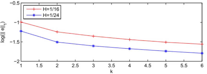
1 1.5 2 2.5 3 3.5 4 4.5 5 5.5 6 −1.5 −1 −0.5 0 k log(|| e h|| 1 ) H=1/16 H=1/24
Fig. 3 The errors decay exponentially with respect to the oversampling parameterk
Table 4 presents the error of PUPM with oversampling parameter k ≈ O(log(1/H ))andm=1,2. The results show the optimal order ofH1error in both cases.
Then, we leteh = uh− ˜uh, also seth = H2, fixm = 1, comparing the errors between the standard two-grid method and our PUPM with different oversampling parameterk atH = 1/16, 1/24. Figure3shows that, for bothH =1/16, 1/24, fromk≥2, log(||eh||1)decrease almost linearly respect tok. This supports that the
error of PUPM decays exponentially with respect to the oversampling parameterk again.
Next, we study the parallel performance of PUPM.
The performance of a parallel algorithm in a homogeneous parallel environment is measured by speedup and parallel efficiency which are commonly calculated by
Sp= T (n1) T (n2) , Ep= n1×T (n1) n2×T (n2) , (4.3)
whereT (n1)andT (n2)(n1< n2)are the wall time of the parallel program usingn1
andn2processors, respectively.
Table5reports the wall times, speed up and parallel efficiency of PUPM with H = 1/16 and km = 2. Here J represents the number of processors, the corre-sponding speedup and parallel efficiency computed withn1=2 in Eq.4.3. Figure4
describes the evolution of the speedup and parallel efficiency with the number of processors respectively. From the table and figure, our PUPM shows a good parallel performance, through it does not reach the optimal parallel efficiency.
Table 5 Wall timeT (J )in seconds, speedupSpand parallel efficiencyEpof PUPM,H=1/16,km=2
J 2 4 8 16 32
T (J ) 170.14 87.65 49.87 31.90 17.38
Sp=T (J )T (2) 1.00 1.94 3.41 5.33 9.79
2 4 8 16 32 2 4 6 8 10 12 14 16 number of processors speedup PUPA Linear speedup 2 4 8 16 32 0.3 0.4 0.5 0.6 0.7 0.8 0.9 1 1.1 1.2 1.3 number of processors parallel efficiency PUPA Linear efficiency
Fig. 4 Left, evolution of speedup T (T (J )2) with number of processors; right, evolution of parallel efficiency
2×T (2)
J×T (J ) with number of processors
5 Conclusions
In this paper, we have designed and analyzed the partition of unity parallel finite ele-ment algorithm and its oversampling strategy. We obtain that, on a uniform coarse meshτH, patches of diameter Hlog(1/H ) are sufficient to preserve the optimal
convergence order. Moreover, the error of this algorithm decays exponentially with respect to the number of layers oversampling. The numerical results and theoretical results keep consistent.
Acknowledgments H. Zheng and L. Song are partially supported by NSF of China with Grant Nos. 11201369, 11271298, 11401332 and NCET, and are partially subsidized by the Fundamental Research Funds for the Central Universities (Grant Nos. 08142003, 08143007).
References
1. Xu, J., Zhou, A.: Local and parallel finite element algorithms based on two-grid discretizations. Math. Comput.69, 881–909 (2000)
2. Bank, R., Holst, M.: A new paradigm for parallel adaptive meshing algorithms. SIAM J. Sci. Comput.
22, 1411–1443 (2000)
3. Bank, R., Holst, M.: A new paradigm for parallel adaptive meshing algorithms. SIAM Rev.45, 291–323 (2003)
4. He, Y., Xu, J., Zhou, A.: Local and parallel finite element algorithms for the Stokes problem. Num. Math.109, 415–434 (2008)
5. He, Y., Xu, J., Zhou, A.: Local and parallel finite element algorithms for the Navier-Stokes problem. J. Comput. Math.24, 227–238 (2006)
6. He, Y., Mei, L., Shang Y., Cui J.: Newton iterative parallel finite element algorithm for the steady Navier-Stokes equations. J. Sci. Comput.44, 92–106 (2010)
7. Shang, Y., He, Y., Kim, D., Zhou, X.: A new parallel finite element algorithm for the stationary Navier-Stokes equations, Finite Elem. Anal. Des.47, 1262–1279 (2011)
8. Liu, Q., Hou, Y.: Local and parallel finite element algorithms for the time-dependent convection-diffusion equations. Appl. Math. Mech. -English Edit.30, 787–794 (2009)
9. Melenk, J., Babuˇska, I.: The partition of unity finite element method: Basic theory and applications. Comput. Methods Appl. Mech. Engrg.139, 289–314 (1996)
10. Babuˇska, I., Melenk, J.: The partition of unity method. Int. J. Numer. Methods Engry.40, 727–758 (1997)
11. Holst, M.: Adaptive numerical treatment of elliptic systems on manifolds. Adv. Comput. Math.15, 139–191 (2001)
12. Holst, M.: Applications of domain decomposition and partition of unity methods in physics and geom-etry (plenary paper). In: Herrera, I., Keyes, D.E., Widlund, O.B., Yates, R. (eds.) Proceedings of the Fourteenth International Conference on Domain Decomposition Methods, Mexico City, Mexico, (2002)
13. Wang, C., Huang, Z., Li, L.: Two-grid partition of unity method for second order elliptic problems. Appl. Math. Mech.-Engl. Ed.29, 527–533 (2008 )
14. Huang, Y., Xu, J.: A partition-of-unity finite element method for elliptic problems with highly oscil-lating coefficients. In: Proceedings for the Work-shop on Scientific Computing, Hongkong, pp. 27–30 (1999)
15. Bacuta, C., Chen, J., Huang, Y., Xu, J., Zikatanov, L.: Partition of unity method on nonmatching grids for the Stokes problem. J. Numer. Math.13, 157–169 (2005)
16. Yu, L., Shi, F., Zheng, H.: Local and parallel finite element algorithm based on the partition of unity for the Stokes problem, SIAM J. Sci. Comput.36, C547–C567 (2014)
17. Zheng, H., Yu, J., Shi, F.: Local and parallel finite element algorithm based on the partition of unity for incompressible flows, submit to J. Sci. Comput.
18. Hou, T., Wu, X., Cai, Z.: Convergence of a multiscale finite element method for elliptic problems with rapidly oscillating coefficients. Math. Comput.68, 913–943 (1999)
19. Nolen, J., Papanicolaou, G., Pironneau, O.: A Framework for Adaptive Multiscale Methods for Elliptic Problems, Multiscale Model. Simul.7, 171–196 (2008)
20. M˚alqvist, A., Peteraseim, D.: Localization of elleptic multiscale problems. Math. Comp.83, 2583– 2603 (2014)
21. Larson, M., Malqvist, A.: Adaptive variational multiscale methods based on a posteriori error esti-mates: energy norm estimates for elliptic problems. Comput. Methods Appl. Mech. Engrg.196, 2313– 2324 (2007)
22. Song, L., Hou, Y., Zheng, H.: Adaptive local postprocessing finite element method for the Navier-Stokes equations. J. Sci. Comput.55, 255–267 (2013)
23. Adams, R.A.: Sobolev Spaces. Academic Press, New York (1975)
24. Ciarlet, P.G., Lions, J.L.: Handbook of Numerical Analysis, Vol. II, Finite Element Methods (Part I). North-Holland, Amsterdam (1991)
25. Ciarlet, P.G.: The finite element method for elliptic problems SIAM Classics in Appl. Math.40, SIAM, Philadelphia (2002)
26. Bochev, P.B., Dohrmann, C.R., Gunzburger, M.D.: Stabilization of low-order mixed finite elements for the stokes equations. SIAM J. Numer. Anal.44, 82–101 (2006)
27. Xu, J.C.: Two-grid discretization technique for linear and nonlinear PDEs. SIAM J. Numer. Anal.33, 1759–1777 (1996)