arXiv:2012.10327v1 [math.OC] 18 Dec 2020
(will be inserted by the editor)
Solving a new type of quadratic optimization problem
having a joint numerical range constraint
Huu-Quang Nguyen · Ruey-Lin Sheu · Yong Xia
Received: date / Accepted: date
Abstract We propose a new formulation about quadratic optimization problems. The objective functionF(f(x), g(x)) is given as composition of a quadratic function F(z) with twon-variate quadratic functionsz1=f(x) andz2=g(x).In addition, it incorporates with a set of linear inequality constraints in z = (z1, z2)T,while having an implicit constraint thatz belongs to the joint numerical range of (f, g). The formulation is very general in the sense that it covers quadratic programming with a single quadratic constraint of all types, including the inequality-type, the equality-type, and the interval-type. Even more, the composition of “quadratic with quadratics” as well as the joint numerical range constraint all together allow us to formulate existing unsolved (or not solved efficiently) problems into the new model. In this paper, we solve the quadratic hypersurfaces intersection problem (QSIC) proposed by P´olik and Terlaky; and the problem (AQP) to minimize the absolute value of a quadratic function over a quadratic constraint proposed by Ye and Zhang. We show that, whenF(z) and the joint numerical range constraint are both convex, the optimal value of the convex optimization problem can be obtained by solving an SDP followed from a new development of the S-procedure. The optimal solution can be approximated by conducting a bisection method on [0,2π]. On the other hand, if the joint numerical range off(x) andg(x) is non-convex, the respective quadratic matrices of f(x) and g(x) must be linearly dependent. The linear dependence property enables us to solve (QSIC) and (AQP) accordingly by elementary analysis.
Huu-Quang Nguyen
Institute of Natural Science Education, Vinh University, Vinh, Nghe An, Vietnam Department of Mathematics, National Cheng Kung University, Tainan, Taiwan E-mail: [email protected]
Ruey-Lin Sheu
Department of Mathematics, National Cheng Kung University, Tainan, Taiwan E-mail: [email protected]
Yong Xia
LMIB of the Ministry of Education, School of Mathematics and System Sciences, Beihang University, Beijing 100191, China
Keywords QCQP, Joint numerical range, S-procedure, Hidden convexity, Intersection of quadratic hypersurfaces, Absolute value of a quadratic function.
1 Introduction
The minimization problem considered in this paper takes the following form:
(Po4)
v(Po4) = inf
(x,z)∈Rn×R2F(z)
s.t. z1a+z2b−c≤0,
z∈C={(f(x), g(x))|x∈Rn}, where a, b, c∈ Rm; f(x) = xTP x+pTx+p0, g(x) = xTQx+qTx+q0 are real-valued quadratic functions ofn-variables with symmetric matricesP, Q;p, q∈Rn andp0, q0∈R.The objective function is a two-variate polynomial inz= (z1, z2)T :
F(z) =zTΘz+ηTz (1)
=θ1z12+ 2θ2z1z2+θ3z22+η1z1+η2z2, with the coefficientsθ1, θ2, θ3, η1, η2∈R.
The model (Po4) has a very special implicit constraint set
C={(f(x), g(x))|x∈Rn}. (2) It is the joint numerical range of two quadratics f and g, which, in general, is a non-convex set. Even if C is convex, since it is not described specifically by convex functions (note that bothf, gcould be non-convex), the problem (Po4) is still not easy to tackle. One of the major contributions in this paper is to show that, when F and the joint numerical range constraintC are both convex, the (abstract)1convex optimization problem can be solved by an SDP followed from a new development of theS-procedure. In this case, (Po4) belongs to the hidden convex optimization [19].
The model (Po4) also has a nice extensibility so that it can be tailored to describe many existing quadratic optimization problems and creates more new ones. By writing the implicit constraintz∈Cexplicitly into a kind of quadratically constrained quadratic problems (abbreviated as (QCQP) in literature) inRn+2:
v(Po4) = inf (x,z)∈Rn ×R2F(z) s.t. f(x)a+g(x)b−c≤0; f(x)−z1= 0; g(x)−z2= 0, (3)
we see, in the following examples, thataf(x) +bg(x)−c≤0 can be used to model quadratic inequality/equality constraints with suitable choices of a, b, c, while f(x)−z1= 0, g(x)−z2= 0 used for perturbations of the values inf(x) andg(x) to give meaningful applications. Interesting examples include
1 Some researchers use the term “abstract” to describe the convex problem which minimizes a convex function over a convex set, while the convex set might not be described by convex functions with inequalities. The case we face here falls into the category.
(i) Whenθ1=θ2 =θ3= 0, η1= 1, η2 = 0, a= 0, b= 1, c= 0,the model (Po4) is reduced to a quadratic program with a single quadratic inequality constraint (abbreviated as (QP1QC) in literature):
(QP1QC) xinf∈Rnf(x)
s.t. g(x)≤0, which has been well studied in [7, 9, 23].
(ii) When θ1 = θ2 =θ3 = 0, η1 = 1, η2 = 0, a = (0,0)T, b= (1,−1)T, c = (0,0)T, (Po4) becomes a quadratic program with a single quadratic equality constraint (abbreviated as (QP1EQC) in literature):
(QP1EQC) xinf∈Rnf(x)
s.t. g(x) = 0. See [11, 21] for a complete solution to (QP1EQC).
(iii) Whenθ1=θ2=θ3= 0, η1= 1, η2 = 0, a= (0,0)T, b= (1,−1)T, c= (β,−α)T andm = 2, (Po4) becomes generalized trust region subproblem (abbreviated as (GTRS) in literature):
(GTRS) x∈infRnf(x)
s.t. α≤g(x)≤β. For discussions on (GTRS), please refer to [7, 11, 16]. (iv) The double well potential problems (DWP) in [1, 20]:
(DWP) min x∈Rn 1 2 1 2kBx−ck 2 −d 2 +1 2x T Ax−uTx
can be represented by (Po4), too. Just chooseθ1= 1, θ2=θ3= 0, η1= 0, η2= 1, a=b=c= 0,and letf(x) = 1 2√2kBx−ck 2, g(x) = −d2kBx−ck 2+1 2x TAx − uTx+d 2 2 .
(v) (Not solved before) In computer graphics, it is fundamental to check whether two quadratic surfaces in 3D Euclidean space intersect and to compute the in-tersection curve if they do. See [6, 17, 18]. P´olik and Terlaky [9] then posed the general quadratic intersections problem in Rn. They ask “Let f(x) = xTP x+pTx+p0= 0, g(x) =xTQx+qTx+q0= 0be two quadric hypersurfaces.
Can we determine whether or not the two hypersurfaces intersect without actually computing the intersections?” In fact, we may further assume that the input data (P, p, p0) and (Q, q, q0) are contaminated by various noises and model the general quadratic intersections problem by the following nonlinear least squares model: (QSIC) inf (x,z)∈Rn×R2(z1) 2+ (z2)2 s.t. ( xTP x+pTx+p0−z1= 0, xTQx+qTx+q0−z2= 0. (4)
Obviously, (QSIC) is a special form of (3) with a =b = c= 0.To our best knowledge, (QSIC) has not been solved before.
(vi) (Not solved efficiently before) Ye and Zhang in [23] proposed to minimize the absolute value of a quadratic function over a quadratic constraint as follows:
(AQP) xinf∈Rn|x
TP x+pTx+p0
| s.t. xTQx+qTx+q0
≤0. Note that (AQP) can be equivalently modeled as
inf
x∈Rn(x
TP x+pTx+p0)2 s.t. xTQx+qTx+q0≤0,
which is again a special type of (Po4) with θ1 = 1, θ2 = θ3 = 0,η1 = η2 = 0, a=c= 0, b= 1.
In [23], (AQP) was formulated as a quadratic optimization problem subject to two quadratic constraints as follows:
mint
s.t. xTQx+qTx+q0≤0, −t≤xTP x+pTx+p0≤t,
and it was suggested to find the optimal valuet∗ with the bisection method.
The procedure requires to conduct the following feasibility check for (many) fixedt≥0:
(AQP-Feas) xinf∈Rnx
TQx+qTx+q0
s.t.−t≤xTP x+pTx+p0≤t.
which is a type of (GTRS) (see case (iii) above). The entire procedure in [23], though polynomially implementable, is very cumbersome due to having to execute an excessive number of SDP’s. Fortunately, our new method in this paper can resolve (AQP) by at most two SDP’s without any assumption (v.s. both primal and dual Slater conditions were assumed in [23]).
The above examples confirm that (Po4) can be widely used in modelling many quadratic optimization problems, but, to solve it in the most general case is diffi-cult. Interestingly, we show that, under the convexity assumptions:
- Θ= θ1 θ2 θ2 θ3 0; (5)
- the joint numerical rangeC={(f(x), g(x))|x∈Rn}is convex, (6) optimal value (Po4) can be solved by solving an (SDP). Given the convexity (5)-(6), the key is to use the separation theorem for developing a new type of S -procedure (Theorem 1 in Sect. 2).
The S-procedure raises the question “when a quadratic function (think it as an objective function) restricted to a set described by quadratic functions (constraint) can be non-negative?” Since it can transform a quadratic optimization problem equivalently to a family of feasibility problems and relates to Lagrange duality, it has become one of the fundamental tools in control theory and optimization. To survey the results before 2006, please refer to [4, 9]. Historically, if the constraint
consists of just a single quadratic function, people refer it asS-Lemma. If there are at least two quadratics in the constraint set, people call it theS-procedure2.
In literature, only theS-lemma was studied completely with a necessary and sufficient condition. It includes three complete versions: the classical S-Lemma proved in 1971 by Yakubovich ([22]); theS-lemma with equality proved in 2016 by Xia et. al ([21]); and the S-Lemma with interval bounds proved in 2015 by Wang et. al ([16]). On the other hand, a complete version of theS-procedure for two or more quadratic functions remains open even for two quadratic forms. Our result in this paper (Theorem 1) is an incomplete version of theS-procedure with m+2 quadratic constraints under convexity assumptions (5) and (6),but it suffices to solve (QSIC) and (AQP) completely.
To apply the newS-procedure, we need to know in advance whether the joint numerical range Cis convex. By Theorem 4.16 in [2], it is known that Ccan be non-convex only when the two matricesP, Qare linearly dependent. We thus solve the two problems (QSIC) and (AQP) by dividing them into two cases:
– Suppose{P, Q}are linearly independent;Cis convex. In this case, (QSIC) and (AQP) can be viewed as a kind of (Po4) satisfying conditions (5) and (6).The complete solution procedure is stated in Section 3.
– IfP=t∗Q(orQ=t∗P), by elementary analysis, we show that (QSIC) can be
reduced to (QP1EQC) (see (ii) above), while (AQP) can be reduced to finding all the solutions to a KKT system.
2 Preliminary: A new S-procedure
Letf(x) =xTP x+ 2pTx+p0, g(x) =xTQx+ 2qTx+q0andF:R2→Rbe defined as in (1). Givenγ∈R,we have the following new type ofS-procedure.
Theorem 1 Under conditions(5)and(6), the following two statements are equivalent:
(G1) (∀x∈Rn, z∈R2)f(x)−z1= 0, g(x)−z2= 0, z1a+z2b≤c ⇒ F(z)−γ≥0. (G2) (∃α, β ∈ R, µ ∈ Rm+) such that F(z)−γ+α(f(x)−z1) +β(g(x)−z2) + µT(z1a+z2b−c)≥0, ∀(x, z)∈Rn×R2.
Proof Note that (G2) ⇒ (G1) is trivial. We only prove that (G1) ⇒ (G2). By condition (6), C = D1 = {z ∈ R2| z1 = f(x), z2 = g(x), x ∈ Rn} is convex. Obviously,D2={z∈R2|z1a+z2b≤c}is convex so thatD1∩D2is convex, too. By (G1),
F(z)−γ≥0∀z∈D1∩D2, which implies that
(D1∩D2)∩D3=∅, where
D3:={z∈R2|F(z)−γ <0}. By condition (5),F is convex, soD3 is an open convex set.
2 Some people might prefer not to distinguishing the two terms betweenS-lemma andS -procedure though.
Let {z :vTz = ¯γ}, with v = (¯α,β)¯T, separate D1∩D2 from D3. Since D3 is open, we assume, without loss the generality, that
¯
αz1+ ¯βz2+ ¯γ≥0, ∀z∈D1∩D2, (7) ¯
αz1+ ¯βz2+ ¯γ <0, ∀z∈D3. (8) From (8), ¯αz1+ ¯βz2+ ¯γ≥0⇒ F(z)−γ ≥0.By S-lemma, there existst≥0 such that
F(z)−γ−t(¯αz1+ ¯βz2+ ¯γ)≥0, ∀z∈R2. (9) Ift= 0, chooseα=β= 0, µ= 0. Then, (G2) holds.
Ift >0, by (7), the following system is unsolvable: tαz¯ 1+tβz¯ 2+t¯γ <0, z1a+z2b−c≤0, z∈D1.
By the Farkas theorem (see [12, Theorem 21.1], [14, Section 6.10 21.1], [9, Theorem 2.1]), there existsµ∈Rm+ such that
tαz¯ 1+tβz¯ 2+t¯γ+µT(z1a+z2b−c)≥0, ∀z∈D1. Equivalently, there isµ≥0 such that,∀x∈Rn,
t¯αf(x) +tβg(x) +¯ t¯γ+µT(f(x)a+g(x)b−c)≥0. Let
α=µTa+t¯α, β=µTb+tβ.¯ (10) Then,∀x∈Rn,one has:
t¯αf(x) +tβg(x) +¯ t¯γ+µT(f(x)a+g(x)b−c)≥0 ⇔(µTa+t¯α)f(x) + (µTb+tβ)g(x) +¯ t¯γ−µTc≥0
⇔αf(x) +βg(x) + (µTa+t¯α−α)z1+ (µTb+tβ¯−β)z2+t¯γ−µTc≥0 (by(10)) ⇔α(f(x)−z1) +β(g(x)−z2) +µT(z1a+z2b−c)≥ −t¯αz1−tβz¯ 2−t¯γ. (11)
Finally, we combine (9) with (11) to obtain (G2).
As for condition (6), there is an easy-to-verify sufficient condition as follows. Theorem 2 (Theorem 4.16 in [2]) If {P, Q} are linearly independent, the joint numerical rangeCdefined by (2)is a convex set inR2.
In the following, we give two examples to show that conditions (5) and (6) cannot be omitted from Theorem 1.
Example 1 Letf(x) =x1+x2, g(x) = 2x2
1−x22, F(z) = 4z21+z2 anda=b=c= γ = 0.Note thatF(z) is convex and condition (5) holds. However, condition (6) is violated since the joint numerical range
C={z∈R2|z2≥ −2z12} is not convex. See [10, Example 3.1].
It can be verified thatz1=x1+x2andz2= 2x21−x22imply that F(z)−0 = 4(x1+x2)2+ (2x21−x22) = 6x21+ 8x1x2+ 3x22≥0. Therefore, (G1) holds. On the other hand,
F(z)−0 +α(f(x)−z1) +β(g(x)−z2)
= 4z21+z2+α(x1+x2−z1) +β(2x21−x22−z2)≥0 holds if and only if
M = 2β 0 0 0 α/2 0 −β 0 0 α/2 0 0 4 0 −α/2 0 0 0 0 (1−β)/2 α/2 α/2 −α/2 (1−β)/2 0 0.
To makeM0,we needβ= 0. However, it leads to
0 (1−β)/2 (1−β)/2 0 = 0 1/2 1/2 0 60
and thus (G2) fails.
Example 2 Let f(x) =x21, g(x) = x22, andF(z) = 2z1z2; a = b = c= γ = 0. By Theorem 2, condition (6) holds. However, condition (5) is clearly violated.
Note thatz1=x21andz2=x22 imply thatF(z)−0 =x21x22≥0.Therefore (G1) holds. On the other hand,
F(z)−0 +α(f(x)−z1) +β(g(x)−z2) = 2z1z2+α(x21−z1) +β(x22−z2)≥0 holds if and only if
M = α 0 0 0 0 0 β 0 0 0 0 0 0 1 −α 2 0 0 1 0 −β 2 0 0 −α 2 −β 2 0 0.
However, this is impossible since
0 1 1 0
60.Then, (G2) fails.
3 Solving (Po4) under conditions (5) and (6) 3.1 Computing the optimal valuev(Po4)
Applying the new S-procedure in Theorem 1, we show that the optimal value v(Po4) under conditions (5) and (6) can be obtained by solving an SDP.
Theorem 3 Under conditions (5)and (6), the optimal value of (Po4), v(Po4),can be computed by v(Po4) = sup γ, α, β∈R µ∈Rm+ γ|M0 , (12) whereM ∈R(n+3)×(n+3) is θ1 θ2 θ2 θ3 [0]2×n µTa+η 1−α 2 µTb+η 2−β 2 [0]n×2 αP+βQ αp+βq µTa+η 1−α 2 µTb+η 2−β 2 αp T+βqT αp 0+βq0−µTc−γ , (13) where[0] = (0ij)2×n with0ij = 0∀i, j.
Proof Since (Po4) can be formulated as (3), we have
v(Po4) = inf (x,z)∈Rn×R2F(z) s.t. f(x)a+g(x)b−c≤0 f(x)−z1= 0 g(x)−z2= 0 = sup γ (x, z)∈Rn×R2 F(z)< γ z1a+z2b≤c f(x) =z1 g(x) =z2 =∅ = sup γ, α, β∈R µ∈Rm+ γ|F(x, z)≥0∀(x, z)∈Rn×R2 , (14)
whereF(x, z) =F(z)−γ+α(f(x)−z1) +β(g(x)−z2) +µT(z1a+z2b−c), and the last equality in (14) holds by Theorem 1. Note thatF(x, z)≥0 can be written as a linear matrix inequality (12) with a matrixM defined in (13).
To illustrate Theorem 3, we provide a numerical example below.
Example 3 Let P = 1 0 0 0 2 0 0 0 3 , p= 0 1 1 , p0 = 7, Q= 1 −2 2 −2 1 3 2 3 1 , q = 1 2 3 , q0= 2,Θ= 1 0 0 2 , η1 η2 = 1 2 ,a=b=c= 0.The SDP (12) becomes: max γ, α, β∈R γ|M 0 , whereM is 1 0 0 0 0 1−α 2 0 2 0 0 0 2−β 2 0 0 α+β −2β 2β β 0 0 −2β 2α+β 3β α+ 2β 0 0 2β 3β 3α+β α+ 3β 1−α 2 2−β 2 β α+ 2β α+ 3β 7α+ 2β−γ .
Remark 1 The computational experiment was conducted in Matlab version R2016a running on a PC with Core i5 CPU and 8G memory. The SDP program (12) is modeled by CVX 1.21 [3] and solved by SDPT3 within CVX.
3.2 Solving for an optimal solution of (Po4)
In general, problem (Po4) under conditions (5) and (6) may not have an optimal solution. First, it can be unbounded from below. For example, letf(x) =x21, g(x) = x22,F(z) =z12−z2, a =b= c= 0. Then both conditions (5) and (6) hold. It is easy to see that
v(Po4) = inf x∈R2 n x41−x22 o =−∞.
Secondly, (Po4) may be bounded but not attainable. For example, letf(x) =x21, g(x) =x1x2−1, F(z) =z12, a=c= (0,0)T, b= (1,−1). Then (Po4) becomes
inf
x∈R2x 4 1
s.t. x1x2−1 = 0.
The optimal value is zero, but there exists nox∈ {x|x1x2= 1}such thatx41= 0. Even if the optimal value v(Po4) is attained at somex∗,we emphasize that it
is generally not easy to solvex∗ from the related SDP optimal solution. Ideally,
we can use the following procedure for obtainingx∗.
Algorithm 1 Solve an optimal solutionx∗ to(Po4)under conditions (5)-(6). Step 1:Compute the optimal valuev(Po4) by solving the (SDP) in (12). Step 2:Solvez∗∈R2 that satisfies
F(z∗) =v(Po4); z∗ 1a+z∗2b≤c; z∗∈C, (15)
whereC is the joint numerical range defined by (2). Step 3:Solvex∗∈Rn that satisfies
f(x∗) =z∗ 1, g(x∗) =z∗ 2. (16)
Note that Step 3 is to solve a simultaneous system of two quadratic equations. Theoretically, it is known that a solution to a system of k quadratic equations, k fixed, can be found in polynomial time. See, e.g., the paper by Grigoriev and Pasechnik in 2005 [5]. However, their procedure appears to be difficult for imple-mentation. In practice, we suggest to use the Newton method for finding the root x∗ in (16).
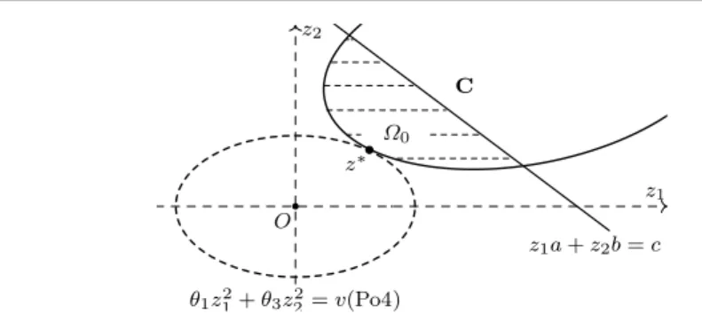
Let us focus on Step 2 in Algorithm 1. Under condition (5), F(z) is a convex function. Then, {z ∈ R2| F(z) = v(Po4)} is either an ellipse, a parabola, or a pair of parallel straight lines inR2, whose forms are either F(z) = θ1z12+θ3z22; F(z) =θ1z21+η2z2, η26= 0 orF(z) =θ1z21, respectively. Figure 1 depicts the case
θ1z21+θ3z22=v(Po4) C z∗ Ω0 z1a+z2b=c z1 z2 O
Fig. 1 Graphic representation for the subproblem (15).
forF(z) =θ1z21+θ3z22 (in black dash), while the set (in stripes bounded by solid curves)
Ω0=C∩ {z∈R2|z1a+z2b≤c} (17) is also convex under condition (6). The intersection
z∗∈Ω
0∩ {z∈R2|F(z) =v(Po4)}
is the required solution for the subproblem (15). Below we propose a type of bisection method on [0,2π] for computing an approximate solution ¯zofz∗.
For simplicity, let us assume thatF(z) =z21+z22for Algorithm 2 below. Given ǫ >0 and suppose in Step 1 of Algorithm 1 we obtain ¯v as an approximate value ofv(Po4) by solving the SDP in (12) such that
¯
v∈[v(Po4), v(Po4) +ǫ/2]. (18)
Algorithm 2 Implementation of Step 2 in Algorithm 1, assuming F(z) =z12+z22. Step 2.1:LetΩ0 as in (17) andǫ, v¯as in (18). Setl0:= 0, u0:= 2π, k:= 0. Step 2.2:Setϕk+1:=
lk+uk
2 and
Ωk+1 :=Ωk∩ {z∈R2|(sinϕk+1,−cosϕk+1)z≥0}.
Solve the following problem by formulating it as an SDP in the form of (12): vk+1= inf
F(z)
z∈Ωk+1 .
Step 2.3:Test whetherz∗ belongs toΩ k+1: – Ifvk+1≤v(Po4),setuk+1:=ϕk+1, lk+1:=lk. – Otherwise, setuk+1:=uk, lk+1:=ϕk+1 and
Ωk+1:=Ωk∩ {z∈R2|(sinϕk+1,−cosϕk+1)z≤0}. Step 2.4:Setk:=k+ 1.If|uk−lk|>arccos
√ ¯ v √ ¯ v+ǫ/2,go to Step 2.2. Otherwise, set ˇz= (√¯vcosuk,√v¯sinuk),ˆz= (√¯vsec22πkcoslk,
√ ¯
vsec22πksinlk).
Step 2.5:Test whether [O,z]ˇ ∩Ω06=∅or [O,z]ˆ ∩Ω06=∅:
– if [O,z]ˇ ∩Ω06=∅(Fig. 2), find a point ¯z in {z : ˇz2z1−zˇ1z2= 0} ∩Ω0 nearest toO(if [O,ˆz]∩Ω06=∅, find a point ¯z in{z: ˆz2z1−zˆ1z2= 0} ∩Ω0 nearest to O). Report ¯z as an approximate solution ofz∗.
– Otherwise (Fig. 3): if [O,z]ˇ ∩Ω0 = ∅ and [O,ˆz]∩Ω0 = ∅, find a point ¯z in {z: ˇz1z1+ ˇz2z2= ¯v} ∩Ω0nearest to ˇz.
z1 z2 z∗ ˇ z ¯ z Ω0 O z1a+z2b=c whereϕ≤arccos√√¯v ¯ v+ǫ/2 z2 1+z22= ¯v∈[v(P o4), v(P o4) +ǫ/2] ϕ
Fig. 2 Graphic representation for the subproblem (15): [O,zˇ]∩Ω06=∅.
z1 z2 z∗ ˇ z ˆ z ¯ z Ω0 O ˇ z1z1+ ˇz2z2= ¯v z2 1+z22= ¯v∈[v(P o4), v(P o4) +ǫ/2] z1a+z2b=c whereϕ≤arccos√√¯v ¯ v+ǫ/2 ϕ
Fig. 3 Graphic representation for the subproblem (15): [O,zˇ]∩Ω0=∅and [O,ˆz]∩Ω0=∅.
3.2.1 Analysis for Algorithm 2
At the first iteration of Algorithm 2, we use the midpointϕ1=π∈[0,2π] to divide the feasible setΩ0 of (Po4) into two parts:
Ω0∩ {z∈R2|z2≥0}andΩ0∩ {z∈R2|z2≤0} and then solve
v1= inf{F(z)|z∈Ω0, z2≥0}, which is certainly a type of (Po4).
Ifv1≤v,¯ we setΩ1=Ω0∩ {z∈R2|z2≥0}and then updateu1=ϕ1=πwith l1 =l0 unchanged. Otherwise, set Ω1= Ω0∩ {z ∈R2| z2 ≤0}.Set l1 = ϕ1 =π whereas keepingu1=u0 as the same. At the next iteration,Ω1is further divided into two parts by either of the midpointsϕ2=π/2∈[0, π] orϕ2= 3π/2∈[π,2π]. This is equivalent to adding a new cutz1≥0 toΩ1. We solve
infnF(z)|z∈Ω1∩ {z∈R2|z1≥0}
o
to determine whether (z∗
1, z2∗)T lies inΩ1∩ {z ∈R2|z1≥0}or not. If affirmative, we set Ω2= Ω1∩ {z ∈R2|z1 ≥0}.Otherwise, set Ω2 = Ω1∩ {z ∈R2|z1 ≤0}. Update the search interval [l2, u2] accordingly. At the third iteration, the setΩ2 is divided into two parts by the line (sin(ϕ3),−cos(ϕ3))z= 0 where the midpoint ϕ3 is eitherπ/4, or 3π/4, or 5π/4, or 7π/4.
In general, at thekthiteration, Algorithm 2 divides [0,2π] into 2kparts. More-over, an optimal solutionz∗ at step 2 of Algorithm 1 is located inΩ
k,which is a
very narrow sector of arc angle 2π/2k intersecting withΩ0. The stopping criterion requires the angle to be smaller than a preset constant, say 2π/2k≤arccos√√v¯
¯
v+ǫ/2. Therefore the number of steps necessarily to achieve this is
k∗(¯v, ǫ) = log2 2π arccos√√v¯ ¯ v+ǫ/2 + 1, (20)
where [t] is the integer part of the real numbert.
When the number of the bisection steps k arrivesk∗(¯v, ǫ), we choose the
fol-lowing two points from the boundary of the sector (see Step 2.4): ˇ z= (√¯vcosuk,√v¯sinuk)∈ {z∈R2|F(z) =z12+z22= ¯v}, ˆ z= (√¯vsec (2π/2k) cosuk, √ ¯ vsec (2π/2k) sinuk).
Notice that both points ˇz,zˆlie on the line{z: ˇz1z1+ ˇz2z2= ¯v},which is tangent to the circle{z∈R2|F(z) =z12+z22= ¯v}at ˇz.Moreover, for allξ∈[ˇz,z],ˆ
√ ¯ v=kzˇk ≤pF(ξ)≤ kˆzk=√v¯sec2π 2k ≤ √ ¯ v· p ¯ v+ǫ/2 √ ¯ v ≤ p v(Po4) +ǫ. That is, F(ξ)≤v(Po4) +ǫ, ξ∈[ˇz,z].ˆ (21) Then, depending on the configuration ofΩ0,the two segments [Oˇz] and [Oˆz] may (Fig. 2) or may not (Fig. 3) intersectΩ0.
- If either [O,z]ˇ ∩Ω0 6= ∅ or [O,ˆz]∩Ω0 6= ∅, say [O,ˇz]∩Ω0 6= ∅, Algorithm 2 finds ¯z in {z : ˇz2z1−ˇz1z2 = 0} ∩Ω0 nearest to O. See Fig. 2. Since the line {z: ˇz2z1−zˇ1z2= 0}passes bothOand ˇz,there is
v(Po4) =F(z∗)≤F(¯z)≤F(ˇz) = ¯v≤v(Po4) +ǫ
2. (22)
Similarly, if [O,z]ˆ ∩Ω06=∅, Algorithm 2 finds ¯z such that, by (21),
v(Po4) =F(z∗)≤F(¯z)≤F(ˆz)≤v(Po4) +ǫ. (23)
In any case, we have
v(Po4)≤F(¯z)≤v(Po4) +ǫ. (24) - On the other hand, if both [O,ˇz]∩Ω0 and [O,z]ˆ ∩Ω0 are empty, Algorithm 2 requires to find a point ¯z in{z: ˇz1z1+ ˇz2z2= ¯v} ∩Ω0 nearest to ˇz (see Fig. 3). The following proposition shows that, when Ω0 is either unbounded or contains an interior point, such a nearest point ¯z always exists.
Proposition 1 Letz,ˇzˆbe defined as in Step 2.4 of Algorithm 2. Suppose, at Step 2.5 of Algorithm 2, there happen that[O,ˇz]∩Ω0=∅and[O,z]ˆ ∩Ω0=∅.
- IfΩ0is unbounded, then [ˇz,z]ˆ ∩Ω06=∅.
- IfΩ0 contains an interior point, then[ˇz,zˆ]∩Ω06=∅for all sufficiently smallǫ >0
whereǫis defined as in (18).
Proof In considering the triangle∆(Oˇzz),ˆ one hasz∗∈Ω0∩∆(Oˇzz) by Algorithmˆ
2. SinceΩ0is convex and unbounded and the two edges [O,z],ˇ [O,ˆz] of∆(Oˇzz) doˆ not intersect withΩ0, the edge [ˇz,ˆz] must intersect withΩ0. Namely, [ˇz,z]ˆ∩Ω06=∅. Now, ifΩ0 contains an interior pointy′∈Ω0 such that the ballB(y′, r)⊂Ω0
for some r > 0. Let 0< ǫ < r2 with ǫ defined as in (18). From (21), we know kˇzk2≤v(Po4) +ǫandkzˆk2≤v(Po4) +ǫso that the triangle∆(Oˇzz) is containedˆ in the ball of centerOwith radiusp
v(Po4) +ǫ≤p
v(Po4)+√ǫ <pv(Po4)+r.On the other hand, for eachy∈B(y′, r)⊆Ω0, one haskyk ≥ kz∗k=p
v(Po4),which implies thatky′k ≥p
v(Po4) +r.Hence,y′∈Ω0 lies outside the triangle∆(Oˇzz)ˆ
whereas z∗ ∈ ∆(Oˇzˆz). Due to the convexity of Ω0, the segment [z∗, y′] ⊂ Ω0.
However, our assumption assumes that [O,z]ˇ ∩Ω0=∅and [O,z]ˆ ∩Ω0=∅so that [ˇz,z]ˆ ∩[z∗, y′]6=∅. The result of this proposition follows immediately.
Hence, with mild assumptions, see Proposition 1, ¯zalways exists and ¯zbelongs to the segment [ˇz,ˆz], so by (21) we haveF(¯z)≤(Po4) +ǫ.
In summary, we have the following result.
Theorem 4 Suppose F(z) = z21 +z22 and that Step 1 in Algorithm 1 returns an approximate optimal value ¯v ∈[v(Po4), v(Po4) +ǫ/2] for a sufficiently smallǫ >0.
Assume that the feasible domain of problem (Po4),Ω0, is either unbounded or contains
an interior point. Then, Algorithm 2 terminates after k∗(¯v, ǫ) (defined as in (20)) number of bisection steps with an approximate solution ¯z ∈ Ω0 such that v(Po4) ≤ F(¯z)≤v(Po4) +ǫ.
3.2.2 Discussion on Step 2.5 of Algorithm 2
To determine whether ˇz= (√¯vcosuk,√v¯sinuk) (the same for ˆz) obtained in Step
2.4 of Algorithm 2 satisfies the condition [Oˇz]∩Ω06=∅, we observe that (see Fig. 2 and Fig. 3) [Oˇz]∩Ω0=∅ ⇐⇒ inf{zˇ1z1+ ˇz2z2: ˇz2z1−zˇ1z2= 0, z∈Ω0}>¯v ⇐⇒ ¯v < inf x∈Rn ˇz1f(x) + ˇz2g(x) s.t. f(x)a+g(x)b−c≤0; ˇ z2f(x)−zˇ1g(x) = 0. (25)
Problem (25) is again a type of (Po4) so that whether or not ˇz ∈ Ω0 can be checked by computing the optimal valuev((25)) of a related SDP as specified in Theorem 3. However, if ˇz 6∈ Ω0, finding a point ¯z in {z : ˇz1z1+ ˇz2z2 = ¯v} ∩Ω0 nearest to ˇz is generally difficult. It amounts to solving a point ¯x∈Rn such that ¯
z1=f(¯x), ¯z2=g(¯x) and ¯z= (¯z1,z2) is a minimum solution to¯
Nevertheless, there is one special case of (26) which we know how to circumvent the difficulty. Whena=b=c= 0,(26) becomes
inf{z2f(x)ˇ −z1g(x) : ˇˇ z1f(x) + ˇz2g(x) = ¯v, x∈Rn}. (27) It is a (QP1EQC). See Introduction. By applying the S-lemma with equality [21] and the standard rank-one decomposition procedure [15], we can obtain an optimal solution ¯xto (27) such that ¯z = (f(¯x), g(¯x))∈Ω0=C is nearest to ˇz. According to Theorem 4, there indeed isv(Po4)≤F(f(¯x), g(¯x))≤v(Po4) +ǫ.
Notice that, in this special case a = b = c = 0, Step 3 in Algorithm 1 for solving a simultaneous quadratic system is not necessary. In the following section, we shall see that the special case suffices to solve the quadratic surfaces intersection problem (QSIC). We thus summarize the discussion into the following theorem. Theorem 5 Leta=b=c= 0; ¯v be an approximate value ofv(Po4) as specified in
(18)andˇz, ˆz be obtained in Step 2.4 of Algorithm 2.
• If [Oˇz]∩Ω0 = ∅ and [Oˆz]∩Ω0 = ∅, we solve x¯ ∈ argmin{zˇ2f(x)−ˇz1g(x) : ˇ
z1f(x) + ˇz2g(x) = ¯v};
•If[Oˇz]∩Ω06=∅, we solve¯x∈argmin{ˇz1f(x) + ˇz2g(x) : ˇz2f(x)−ˇz1g(x) = 0}; •If[Oˆz]∩Ω06=∅, we solve¯x∈argmin{ˆz1f(x) + ˆz2g(x) : ˆz2f(x)−ˆz1g(x) = 0};
where[Oz]∩Ω0 =∅ ⇐⇒ ¯v <inf{z1f(x) +z2g(x) :z2f(x)−z1g(x) = 0, x∈Rn}.
Then, x¯is an approximate optimal solution to (Po4)with F(z) =z21+z22 such that
v(Po4)≤F(f(¯x), g(¯x))≤v(Po4) +ǫ.
4 Applications 4.1 Problem (QSIC)
The problem (QSIC) defined in (4) can be recast in the following form: (QSIC) inf
x∈Rn(x
T
P x+pTx+p0)2+ (xTQx+qTx+q0)2.
It is to determine whether or not the two hypersurfaces,f(x) =xTP x+pTx+p0= 0 andg(x) =xTQx+qTx+q0= 0, intersect. Ifv(QSIC) = 0,orv(QSIC)< ρfor some user-defined smallρ >0 to accommodate possible noises arising from the problem data, the two hypersurfaces are thought to intersect with each other. Otherwise, v(QSIC) gives some sort of measurement as to how far the two hypersurfaces deviate from each other. For this purpose, the optimal valuev(QSIC) suffices to decide the intersection problem. However, problem (QSIC) belongs to the special case that F(z) =z21+z22 anda=b=c= 0.By Theorem 5, we are able to find an approximate solution ¯x which is either a common root of the two quadratic equationsf(x) =g(x) = 0; or can be viewed as a point whose total distance to the two hypersurfacesf(x) = 0 and g(x) = 0 is the least.
We solve (QSIC) by two cases.
Case 1: If{P, Q}are linearly independent, by Theorem 2 and by takingF(z) = z12+z22,a=b=c= 0,we see that (QSIC) is a (Po4) satisfying conditions (5)-(6). In this case, the optimal valuev(QSIC) can be computed by the following (SDP):
γ∗= sup γ, α, β∈R
whereM is 1 0 0 1 [0] −α 2 −β 2 [0]T αP+βQ αp+βq −α 2 − β 2 αp T+βqT αp 0+βq0−γ .
The optimal solution of (QSIC), if attainable, can be computed approximately via Algorithm 1, Algorithm 2 and Theorem 5.
Case 2: If{P, Q}are linearly dependent, sayQ=t∗P.IfP =Q= 0,then (QSIC)
is an unconstrained convex quadratic optimization problem, which can be solved directly. Hence, let us assume thatP6= 0.Then, we multiply the first equation in (4) byt∗and subtract it from the second equation to obtain
( xTP x+pTx+p0−z1= 0, (qT−t∗pT)x+ (q0 −t∗p0) +t∗z1−z2= 0. (28) Define yT = [xT, zT];hT = [qT −t∗pT, t∗,−1];h0=q0−t∗p0; and ¯ A= [0]n×n[0]n×2 [0]2×n I2×2 , P¯= P [0]n×2 [0]2×n[0]2×2 6 = 0.
Then, (QSIC) becomes
infy∈Rn+2 yTAy¯
s.t. yTP y¯ + ¯pTy+p0= 0, hTy+h0= 0,
where ¯pT = [pT,−1,0].By the null space representation, the solution set for the hyperplanehTy+h0= 0 can be written asy=y0+V zfor somez∈Rn+1,where y0 = − h0
hThh and V ∈ R
(n+2)×(n+1) is the matrix basis of
N(h). It implies that (QSIC) is reduced to the following (QP1EQC) problem:
inf
z∈Rn+1 (y0+V z)
TA(y0¯ +V z) (29)
s.t. (y0+V z)TP¯(y0+V z) + ¯pT(y0+V z) +p0= 0, which can be solved by applying the S-lemma with equality. See [21].
4.2 Problem (AQP)
Notice that (AQP) can be equivalently formulated as follows: inf (x,z1)∈Rn×R z12 s.t. ( xTP x+pTx+p0−z1= 0, xTQx+qTx+q0≤0. (30) We again split the discussion into two cases: Case 1:{P, Q}are linearly indepen-dent; Case 2:{P, Q}are linearly dependent.
z1 z2 O z2 1=v(Po4) C (z∗ 1, z∗2) z2= 0 Fig. 4 z1 z2 O z2= 0 z2 1=v(Po4) C (z∗ 1, z∗2) Fig. 5
•Case 1:If{P, Q}are linearly independent, by writing (30) as inf (x,z1)∈Rn×R z21 s.t. z2≤0, f(x) =xTP x+pTx+p0=z1, g(x) =xTQx+qTx+q0=z2, (31)
with F(z) = z21, a = 0, b = 1, c = 0, we see that (AQP) is a (Po4) satisfying conditions (5)-(6). Then, the optimal valuev((31)) can be computed by:
γ∗=v(AQP) = sup γ, α, β∈R γ |M 0 , whereM is 1 0 0 0 [0] −α 2 µ−β 2 [0]T αP+βQ αp+βq −α 2 µ−β 2 αp T +βqT αp 0+βq0−γ .
Although the optimal solution can be computed approximately via Algorithm 1 and Algorithm 2, yet due to F(z) =z21 andz2 ≤0 being simple functions, we can solve it in a better way without resorting to the bisection method.
- First, if γ∗ = v(AQP) = 0, then any optimal solution to the following
(QP1EQC) is an optimal solution to (31).
(QP1EQC) xinf∈Rng(x)
s.t. f(x) = 0.
The solution of (QP1EQC) can be obtained by solving an SDP and a standard matrix rank one decomposition. See [21, 15].
- Secondly, ifγ∗=v(AQP)>0, then one has{z∈R2
|z12< γ∗} 6=∅and
{z∈R2:−pγ∗< z1<pγ∗} ∩ C∩ {z∈R2|z2≤0}
SinceC∩ {z∈R2:z2≤0}is convex, there must be either C∩ {z∈R2|z2≤0} ⊂ {z∈R2|z1≥pγ∗}; or C∩ {z∈R2|z2≤0} ⊂ {z∈R2|z1≤ −p γ∗}.
In the former case, (AQP) is solved by inf{f(x) : g(x)≤0} (see Fig. 4 and 4), while the latter case can be solved by inf{−f(x) :g(x)≤0}. Both problems are (QP1QC).
•Case 2:If{P, Q}are linearly dependent such thatQ=t∗P, we assume that there
exists a minimizer where KTCQ is satisfied. Now, we can use a linear combination to eliminate the matrixQin (31) and get
inf (x,z1)∈Rn ×Rz 2 1 s.t. ( xTP x+pTx+p0−z1= 0, (qT −t∗pT)x+ (q 0−t∗p0) +t∗z1≤0. (32)
Then, we solve an optimal solution, say x∗, to (AQP) (if attainable) by fully
analyzing the KKT system of (32). To this end, let us assume some suitable constraint qualification hold atx∗.
Let λ1 ∈ R, λ2 ≥ 0 be the Lagrange multipliers associated with the two constraints in (32), respectively. The KKT system can be written down as follows:
−2z1=−λ1+λ2t∗; 0 =λ1(2P x+p) +λ2(qT −t∗pT); xTP x+pTx+p0−z1= 0; (qT −t∗pT)x+ (q 0−t∗p0) +t∗z1≤0; λ2 (qT−t∗pT)x+ (q0 −t∗p0) +t∗z1 = 0; λ2≥0. (33)
- Case 1:λ2>0. By the complementary slackness, (qT−t∗pT)x+ (q0
−t∗p0) +
t∗z1= 0.That is, the second inequality constraint in (32) is active. Therefore, to
check whether there are KKT candidates (z∗
1, x∗) associated withλ2>0 satisfying (33), we can instead find optimal solutions (z∗
1, x∗) to the following problem inf (x,z1)∈Rn ×Rz 2 1 s.t. xTP x+pTx+p0−z1= 0; (qT−t∗pT)x+ (q 0−t∗p0) +t∗z1= 0, (34)
which can be reduced to an (QP1EQC) problem as in (29). - Case 2:λ2= 0, then (33) becomes
−2z1=−λ1; 0 =λ1(2P x+p); xTP x+pTx+p0−z1= 0; (qT −t∗pT)x+ (q0 −t∗p0) +t∗z1≤0. (35)
Withλ1=λ2= 0,we havez1= 0 and (35) becomes
(
xTP x+pTx+p0=z1= 0; −(qT−t∗pT)x+ (q0
−t∗p0)≤0. (36)
Since the objective function isz21, any solution of (36) is also a solution of (32). It can be decided by solving the following (QP1EQC):
inf x∈Rn−(q T −t∗pT)x+ (q0 −t∗p0) s.t. xTP x+pTx+p0= 0. (37)
If the optimal value v((37))> 0, then (36) does not have a solution. In this case,λ16= 0, λ2= 0 such that (35) becomes
2z1=λ16= 0; 0 =λ1(2P x+p); xTP x+pTx+p0−z1= 0; (qT−t∗pT)x+ (q0 −t∗p0) +t∗z1≤0. (38) Then, 2P x+p= 0 and z1=xTP x+pTx+p0= 1 2p Tx +p0.
Hence, (38) is reduced to the following linear system in variables (x, z1, λ1)∈Rn+2:
2z1=λ16= 0; 2P x+p= 0; 1 2pTx+p0−z1= 0; (qT−t∗pT)x+ (q0 −t∗p0) +t∗z1≤0. (39)
In summary, when{P, Q}are linearly dependent, we can solve (i) λ2>0 and (34); (ii)λ1=λ2= 0 and (37) withv((37))≤0; and (iii)λ16= 0, λ2= 0 and the linear system (39). The optimal solution of (AQP) will be the valid ones among (i), (ii) and (iii) with the smallest objective valuez12of (AQP).
Example 4 inf x∈R2 −x21+x22+x1 s.t.−x21+x22+ 1≤0. (40) In this example,{P, Q}are linearly dependent witht∗= 1.Using the linear
com-bination witht∗= 1 to eliminateQ, we can write
inf (x,z1)∈R2 ×Rz 2 1 s.t. −x21+x22+x1−z1= 0, −x1+z1+ 1≤0. (41)
Since we are going to utilize the KKT system of (41), we first check the constraint qualification. Notice that,
The two gradients are linearly dependent if and only ifx1=x2= 0. Whenx1= x2= 0, (41) has an empty feasible set{z1= 0, z1≤ −1}=∅.In other words, every optimal solution to problem (40) must be a regular point of the KKT system.
Then, check all the following three cases:
(i) λ2>0.Then, the inequality−x1+z1+ 1≤0 is active so thatx1=z1+ 1.We first solve the (QP1EQC):
inf (z1,x2)∈R×R
z21
s.t. −(z1+ 1)2+x22+ 1 = 0
(42)
to obtain the solutionz∗
1 = 0, x∗1= 1, x∗2= 0 to (42). From the first equation −2z1=−λ1+λ2t∗in the KKT system (33), sincez∗
1 = 0, t∗= 1,we obtain λ1=λ2>0.
From the second equation of (33), (x∗
1, x∗2)T must satisfy 0 = (2P x+p) + (qT −t∗pT
) which is not true as (2P x∗+p) + (qT
−t∗pT) = (
−3,0)T. We conclude that there is no KKT point of (42) withλ2>0.
(ii) λ1=λ2= 0.In this case, the KKT system (33) is reduced to (36), which is
(
−x21+x22−x1=z1= 0;
−x1+z1+ 1≤0. (43) Since (43) guarantees that z1 = 0,any solution to (43), if exists, is an opti-mal solution to (AQP). It is not difficult to see that (43) has infinitely many solutions among which we can choose, for example,z∗
1= 0, x∗1= 1, x∗2= 0. (iii) λ16= 0, λ2 = 0. Dealing with this case might help to find other solutions to
(40). In this case, we need to check the linear system in (39), which is:
2z1=λ16= 0; (−2x1,2x2) + (1,0) = (0,0); z1= x1 2; −x1+z1+ 1≤0. (44)
From the second and the third equation of (44), we getx1= 0.5, x2= 0, z1= 0.25.They do not satisfy−x1+z1+ 1≤0 though. The system (44) does not have a solution, either.
5 Conclusion and Discussion
In this paper, we propose a new type of quadratic optimization problems involving a joint numerical range constraint. There are many natural applications arising from such a formulation. Some applications like the double well potential problem (DWP) [1, 20] were already solved independently, while others like (QSIC) and (AQP) can now be resolved through our new approach. Interestingly, due to the composition of “quadratic with quadratics,” the objective functionF(f(x), g(x)) is
indeed a polynomial of degree 4. We hope that our method can be later extended to solve optimization problems involving quartic polynomials.
Notice that, in Theorem 1, we can replace {f, g} by k quadratic functions {f1,· · ·, fk}. The theoretical results in this paper are still valid (the
implemen-tation can be more complicate though), provided the following conditions are satisfied:
{(f1(x),· · ·, fk(x))|x∈Rn}is convex,
Θk×k0,
where Θk×k defines a quadratic functionf(z) = zTΘk×kz+ηTz of k variables.
It suggests that the convexity of the joint numerical range of {f1,· · ·, fk} is the
central feature for many optimization problems and should be studied carefully in the future.
Acknowledgements
Huu-Quang, Nguyen’s research work was sponsored partially by Taiwan MOST 107-2811-M-006-535 and Ruey-Lin Sheu’s research work was sponsored partially by Taiwan MOST 107-2115-M-006-011-MY2.
Xia’s research was supported by National Natural Science Foundation of China un-der grants 11822103, 11571029, 11771056, and Beijing Natural Science Foundation Z180005.
References
1. Fang, S.C. and Gao, D.Y. and Lin, G.X. and Sheu, R.L. and Xing, W., 2017.Double well potential function and its optimization in the n-dimensional real space- Part 1.Journal of Industrial and Management Optimization, 13, pp. 1291-1305.
2. Flores-Baz´an, F. and Opazo, F., 2016.Characterizing the convexity of joint-range for a pair of inhomogeneous quadratic functions and strong duality.Minimax Theory and its Applications, 1, pp. 257-290.
3. Grant, M. and Boyd, S., 2010.CVX: Matlab software for disciplined convex programming.
Version 1. 21 Web.
4. Derinkuyu, K. and Pinar, M.C¸ , 2006.On the S-procedure and some variants. Mathematical Methods of Operations Research, 64, pp. 55-77.
5. Grigoriev, D. and Pasechnik, D.V., 2005.Polynomial-time computing over quadratic maps i: sampling in real algebraic sets.Computational complexity, 14(1), pp. 20-52.
6. Levin, J., 1979.Mathematical models for determining the intersections of quadratic sur-faces.Computer Graphics and Image Processing, 11, pp. 73-87.
7. Mor´e, J.J., 1993.Generalizations of the trust region problem.Optimization methods and Software, 2(3-4), pp. 189-209.
8. Nguyen H.Q. and Sheu, R. L., 2020. Separation properties of quadratic functions. Avail-able from: https://doi.org/10.13140/RG.2.2.18518.88647.
9. Polik, I. and Terlaky, T., 2006.A survey of the S-lemma.SIAM Review, 49, pp. 371-418. 10. Polyak, B. T., 1998.Convexity of quadratic transformations and its use in control and
optimization.Journal of Optimization Theory and Applications, 99, pp. 553-583. 11. Pong, TK. and Wolkowicz, H., 2014.The generalized trust region subproblem.Journal of
Optimization Theory and Applications, 58, pp. 273-322.
12. Rockefellar, R. T., 1970.Convex analysis.Princeton University Press.
13. Stern, R. and Wolkowicz, H., 1995.Indefinite trust region subproblems and nonsymmetric eigenvalue perturbations.SIAM Journal on Optimization, 5, pp. 286-313.
14. Stoer, J. and Witzgall, C., 1970. Convexity and Optimization in Finite Dimensions.
Springer-Verlag, Heidelberg. I
15. Sturm, J. F., Zhang, S., 2003.On cones of nonnegtive quadratic functions.Mathematics of Operations Research, 28(2), pp. 246–267
16. Wang, S. and Xia, Y., 2015. Strong Duality for Generalized Trust Region Subproblem: S-Lemma with Interval Bounds.Optimization Letters, 9, pp. 1063-1073.
17. Wang, W. and Joe, B. and Goldman, R., 2002.Computing quadric surface intersections based on an analysis of plane cubic curves.Graphic models, 64, pp. 335-367.
18. Wilf, I. and Manor, Y., 1993.Quadric-surface intersection curves: shape and structure.
Computer-Aided Design, 25, pp. 633-643.
19. Xia, Y. 2020.A survey of hidden convex optimization.Journal of the Operations Research Society of China, 8(1), pp. 1-28.
20. Xia, Y. and Sheu, R.L. and Fang, S.C. and Xing, W, 2017.Double well potential function and its optimization in the n-dimenstional real space - Part 2.Journal of Industrial and Management Optimization, 13, pp. 1307-1328.
21. Xia, Y. and Wang, S. and Sheu, R.L., 2016.S-lemma with equality and its applications.
Mathematical Programming Series A, 156(1), pp. 513-547.
22. Yakubovich, V.A., 1971.S-procedure in nonlinear control theory. Vestnik Leningrad Uni-versity (in Russian), 1, pp. 62-77.
23. Ye, Y. and Zhang, S. , 2003.New results on quadratic minimization.SIAM Journal on Optimization, 14, pp. 245-267.
![Fig. 2 Graphic representation for the subproblem (15): [O, ˇ z] ∩ Ω 0 6= ∅ .](https://thumb-us.123doks.com/thumbv2/123dok_us/9027818.2389938/11.892.121.587.120.356/fig-graphic-representation-subproblem-o-ˇ-z-ω.webp)
