Time-domain Beamforming using 3D-microphone arrays
Gunnar Heilmannagfai tech Rudower Chaussee 30
12489 Berlin Germany
Andy Meyerband Dirk Döblerc GFaI
Society for the promotion of applied computer science
Rudower Chaussee 30 12489 Berlin
Germany ABSTRACT
Acoustic measurements inside any cavity are mostly conducted with a view number of microphones. By this means it is possible to gain information about frequencies, orders, sound pressures. However, a space selective analysis is nearly impossible and it is not feasible to find multiple sound sources position in space in a practical way. Traditional beam forming systems with planar microphone arrays do not give comprehensive information about the sound sources inside a cavity such as car interior or an office room.
Therefore, the constituents of the Acoustic Camera of the GFaI were extended by a spherical, acoustically transparent and omni directional array. A new option is to map onto a common 3D-CAD-models of the object of interest, for instance an office or class room. First of all the advantages and disadvantages of 2D- and 3D-mappings will be discussed in the paper. Furthermore, the important issue of positioning an array at first in the coordinate system of the 3D-model and second in the actual cavity which is to be measured will be addressed. The paper discusses the geometric and acoustic properties of microphone arrays which are applicable for complete 3D-measurements and mappings of cavities. A practicable way of determining the array’s position and direction related to the measurement object will be proposed. Several practical experiments will be displayed to underline the methods capability and reliability.
1 INTRODUCTION
Actual commercial Beamforming systems, among them the Acoustic Camera, use a rectangular virtual image plane in order to calculate the run times between microphone array and measurement object (figure 1). This way the surface of the device under test is approximated, and the z-axis of the array is usually oriented perpendicularly to the image plane. The Resolution of an acoustic image is determined by the way the image plane is subdivided into rows and columns, which results in a finite amount of rectangular display details (pixels). The center of each sub area is used to calculate the delays. Sound sources which are placed on a three dimensional device surface will be localized and mapped onto this two dimensional plane.
a
Email address: heilmann@gfaitech.de
b
Email address: meyer@gfai.de
c
Measurement object
z
Mikrophon array
y x
Virtual image plane
Calculating pixel
Figure 1: Conventional beamforming and mapping onto a 2D virtual image plane This method causes two errors: At first the beamformer uses an incorrect focus for most of the pixels. Dependent on array geometry, subsurface structure, frequencies of the sound source and distance between array and object, the calculated level of sound pressure differs from the level calculated with correct focus. Second, by
mapping the (incorrect) calculated sound sources on a two dimensional plane we will get distortions. Sound sources may be localized incorrectly. In most beamforming applications these effects are negligible, but for mapping of interior cavity these effects are noticeable. This effect gets most dramatic in the room and building acoustics application, where the varying depth of the room can be enormous.
2 MAPPING OF 3D SURFACES
To solve these problems, we replace the simple mapping of a virtual plane at a fixed distance by different measurement distances to individual points in a 3D-model surface. Of course, we need a 3D-model of the measurement object, preferably available in a standard CAD *.stl-file format. In many sectors of industries, this precondition is fulfilled in most cases. 3D-models of engines, cars or airplanes usually consist of several hundred thousands of triangles.
In 3D-mappings, the planar virtual surface subdivided in pixels is now replaced by lots of triangles definitely oriented in space and modelling the actual surface of the measurement object. Dependent on the desired acoustic resolution and the given graphical model resolution, those triangles may either be coloured directly or may themselves be subdivided into pixels (texturing). The time delays are now calculated in three-dimensional space for every individual triangle or for every individual sub-pixel of all the triangles, respectively.
Figure 2: Correct focussing of the beamformer to depth structured surface of measurement object
The acoustic map of a 3D-model surface includes only the values from points respectively triangles which are really situated on the surface of the object, in contrast a mapping of a 2D virtual plane often includes calculated points beside the real object. If the beamformer is optimized to avoid sidelobes in the inner region of the visible image field, the mapping onto a 3D object often leads to seemingly better contrast values or to say dynamic range, because sidelobes, normally in the outer region often diminishing image contrast in the 2D case are now excluded from the calculation. On the other hand, if a real acoustic source is present in the image field which is not contained in the 3D-model, it is possible that this source or its sidelobes are erroneously mapped onto the surface of the 3D-model or they are not visible at all. Therefore, it is advisable to accompany every 3D-mapping by an additional 2D-mapping. A typical case of incorrect 3D-mapping is shown in figure 3.
Figure 3: 2D-mapping of a sound source caused by an unfixed mounting (right), the same measurement, but mapped on a 3D-model (left). The result erroneously suggests a noise source situated on the engine (because mounting is not part of the CAD-model), but its mounting post is actually responsible for this noise.
3 MICROPHONE ARRAYS FOR USE INSIDE A CAVITY
In addition to the above mentioned precondition, for mapping of interior we need a suitable microphone array. It is basically possible to generate 3D-mappings with any kind of microphone arrangements, although the quality and the expressiveness of the results will decrease. The following simulations (figures 4, left) show a 3D-mapping on a spherical room (Ø 2m) with a sound source (white noise 0-20 kHz) in front of a 2D ring microphone array. As result we get two sound sources. The first and the correct source is situated in front of the array. The other noise source behind the ring array is a mirror image of the first source. Because of the ambiguities between 3D points and Microphones (we can always find two points on the spherical model surface which have the same distance to all microphones), we do not get a unique solution. This fact has great relevance for measuring outside of acoustic test chambers too.
Figure 4: 3D-mapping of a sound source in front of a ring (left, 12 dB contrast) and on the right hand side (right, 8 dB contrast)
The left figure shows the same situation as in the right figure. Only one modification has been carried out. The position of the noise source changed from the front of the microphone array to the right hand side. Poor geometric cutting conditions result from the position between the noise source and the microphones. It is almost impossible under these terms to locate the source exactly.
Conventional planar arrays with a favored imaging direction are not able to perform undistorted 3D-mappings. The characteristics of the array (frequency response, resolution, side lobes etc.) should be as identical as possible for all directions in space. An array having its microphones equally distributed on a (virtual) spherical surface and with the sensor’s direction vectors perpendicular to this sphere will be adequate.
The frequency range of an array is depending on minimum and maximum distances between the microphones. If we spread microphones on a virtual spherical surface, we need more microphones to get the same frequency range as a planar array. In order to construct a spherical array there are two possible ways: solid sphere or acoustic transparent sphere. A solid sphere is easier in manufacturing. But it has some disadvantages: the sound field will be disturbed, half the number of microphones is shadowed and the surface of the sphere will be generating
reflections and frequency dependent errors in measurement results. Of course, the shadowed microphones also receive the acoustic waves from the noise source because the waves are diffracted around the sphere, but the diffraction and therefore the time delays are frequency dependent. These properties of a solid sphere enforce a calculation of the acoustic map in the frequency domain to correct these errors. The calculation of three dimensional acoustic maps in the frequency domain requires high computational power, and the analysis of non-stationary noise events is difficult and imprecise. Last but not least, the weight of a solid sphere may make the handling difficult. Therefore we use only acoustically transparent arrays.
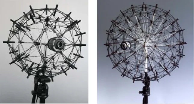
Two examples of spherical transparent arrays are shown in figure 5.
Fig. 5: Spherical acoustically transparent arrays with 48 channels and 120 channels and a built-in video camera
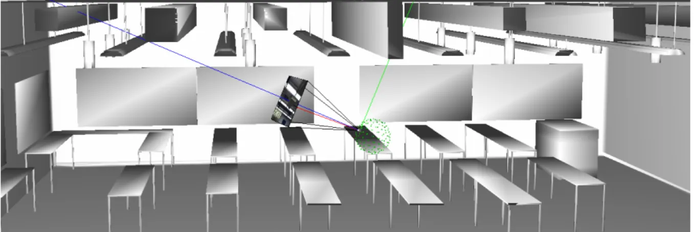
The example in figure 6 shows the employment of such an array. Two sources have been placed in the scene. The first one is situated behind and the second one is situated on the right hand side of the array. Both noise sources (white noise 0-20 kHz) were exactly located on the 3D Model (Ø 2m).
Fig. 6: 3D-mapping of two sound sources behind and on the right hand side from the array
4 PRACTICAL NOISE SOURCE IDENTIFICATION INSIDE A CAVITY
The gfai tech GmbH uses 3D acoustic mapping also as service consultancies for sound localization of cars interiors during development process, in quality control and now also in the field of room and building acoustic. The mapping on 3D objects has to be considered as add on to the standard acoustic tools and has its advantages. In order to show the capability of Time-Domain-Beamforming using 3D-Microphone-Arrays the following examples of acoustic photos show a selection of generated sounds to observe the mapping quality of different kind of noise sources. Chosen were artificial as well as real - broad band, transient and sine like sound sources.
The sources were recorded with a 32, 48 or 120 channel spherical array usually positioned in the centre of each cavity (example in figure 7). Basis for each acoustic mapping were A-weighted and specific high pass filtered signals. For better visualization of the samples, the 3D-mappings are shown in a partial view of the full interior. The dynamic scale of the acoustic color-maps is varying by application and signal form to show the origin of the main sound source(s) clearly.
Figure 7: Position of the microphone array in UM –Class Room 2216
In everyday practise the quality of the mapping varies with application. The method comes to its limit when sources are hidden. Sources can be hidden behind or under panels, ceilings and other objects. Facing these kinds of phenomena not the precise origin of the source will be shown in the image, but a reflection or diffraction of it. Possible room resonance, reflection and diffraction and other possible acoustic behaviour of sources has to be taken into account when interpreting any acoustic 3D-photos. The acoustic maps always represent the sound field as it is measured from the position of the array.
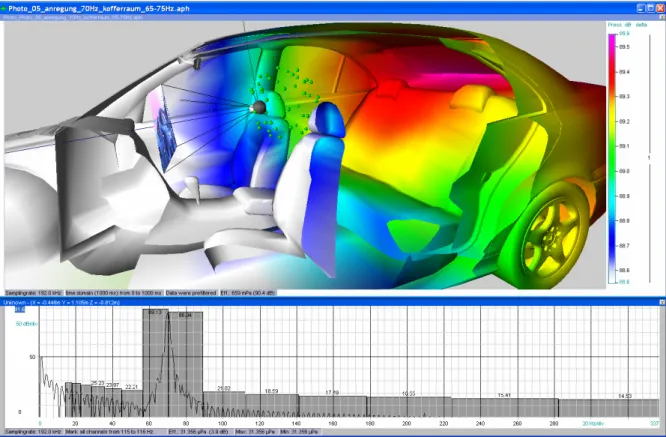
Furthermore the room- and array- geometry influences the resolution especially when low frequencies are of interest. Less dynamic range is a result of these effects. One dB dynamic range is shown in the example of a car interior measurement in figure 8. The main source can still be found correctly and shows surprisingly a source of a 70Hz pure tone. Therefore the recommended mapping frequency-bands are related to the size of the arrays, the sources characteristic and again strongly depend on room- and array- geometry.
Figure 8: pure tone 70Hz from sub woofer in the trunk, passenger side (1dB contrast)
As the sources get more transient and/or more broad band, the source identification becomes easier and easier through this method. In Figure 9 a measurement of a car interior is performed on four poster shaker. Followed by an 800Hz high pass filter the most conspicuous source shown in the time history is base of the calculation.
When measuring in larger cavities the 120 channel sphere was in use. The following examples show an empty office room with some known isolated sources. First test was a common shredder placed in one corner of the room. The shredder can easily be identified as sound source.
Figure 10: measurement in empty office room, testing common shredder (5dB dynamic)
Figure 11: same measurement as in figure 10, showing scene from different angle at 1dB contrast After decreasing dynamic range of the acoustic photo, the built in electric motor is correctly identified on the right hand side of the shredder. During the next measurement a white noise source was placed outside the room. The data was recorded at 96kHz and the signal A-Filtered before creating an acoustic photos in 3D. A strong leakage shows up on centre the upper frame of the top window.
Figure 12: White noise source outside the room, window clo 24dB)
3dB) , a asketball hall and later an entire Football stadium at University of Michigan the
sed (5dB dynamic, peak level at
Figure 13: White noise source outside the room, window tilted (9dB dynamic, peak level at 5 Further test were performed in rooms increasing size. Measuring a class room B
system proofed its capability and reliability.
3 CONCLUSION
Time-domain Beamforming using 3D-microphone arrays is an extremely fast, easy and simple way to find sources inside cavities. Source-characteristic, room-acoustic and array-geometry will set limits to the resolution and display in acoustic pictures. For “Buzz, Squeak and Rattle Tests” or highly transient sources can be best mapped and separated in time and space, when using a high sampling rate of 192 kHz and Zero Padding. Measurements with low frequency sources are generally possible but need to be interpreted with some precaution and the need of validation! The quality of the acoustic maps varies with the number of possible different application.
Generally speaking; very tonal and low frequency sources are mapped with less dynamic range and limited resolution in the acoustic images. Transient and broad band sources map very sharp and with great dynamic range.
4 REFERENCES
[1] D. Döbler, A. Meyer : “Dreidimensionale akustische Kartierungen mit kugelförmigen Mikrofonarrays”, Proceedings of the DAGA 2007, Stuttgart, Germany, (2007)
[2] A. Meyer, D. Döbler: „Noise source localization within a car interior using 3D-microphone arrays“,Proceedings of the BeBeC 2006, Berlin, Germany, (2006)
[3] D.H.Johnson, D.E Dudgeon : „Array Signal Processing. Concepts and Techniques“, PTR Prentice Hall, (1993)
[4] H. van Trees: „Optimum Array Processing“, J. Wiley & Sons, (2002) [5] P.S. Naidu: „Sensor Array Signal Processing“, CRC Press LLC, (2001)