Statistical Methods for Multivariate Meta-analysis of Diagnostic
Tests: An Overview and Tutorial
Xiaoye Ma1, Lei Nie2,a, Stephen R. Cole3, and Haitao Chu1,*
1Division of Biostatistics, School of Public Health, University of Minnesota, Minneapolis, MN
55455
2Division of Biometrics IV, Office of Biometrics/OTS/CDER /FDA, Silver Spring, MD 20993-0002
3Department of Epidemiology, University of North Carolina, Chapel Hill, NC 27599
Summary
In this article, we present an overview and tutorial of statistical methods for meta-analysis of diagnostic tests under two scenarios: 1) when the reference test can be considered a gold standard; and 2) when the reference test cannot be considered a gold standard. In the first scenario, we first review the conventional summary receiver operating characteristics (ROC) approach and a bivariate approach using linear mixed models (BLMM). Both approaches require direct calculations of study-specific sensitivities and specificities. We next discuss the hierarchical summary ROC curve approach for jointly modeling positivity criteria and accuracy parameters, and the bivariate generalized linear mixed models (GLMM) for jointly modeling sensitivities and specificities. We further discuss the trivariate GLMM for jointly modeling prevalence, sensitivities and specificities, which allows us to assess the correlations among the three parameters. These approaches are based on the exact binomial distribution and thus do not require an ad hoc continuity correction. Last, we discuss a latent class random effects model for meta-analysis of diagnostic tests when the reference test itself is imperfect for the second scenario. A number of case studies with detailed annotated SAS code in procedures MIXED and NLMIXED are presented to facilitate the implementation of these approaches.
Keywords
meta-analysis; diagnostic test; gold standard; generalized linear mixed models
1. Introduction
In the medical literature, a diagnostic test commonly refers to a medical test to classify subjects with respect to a (disease) state of interest. Accurate diagnosis plays an important role in the disease control and prevention. Diagnostic test outcomes could be dichotomous, ordinal or continuous. This article only focuses on the dichotomous outcome. The
performance of a binary test is commonly measured by a pair of indices such as sensitivity
HHS Public Access
Author manuscript
Stat Methods Med Res
. Author manuscript; available in PMC 2014 December 26.Published in final edited form as:
Stat Methods Med Res. 2016 August ; 25(4): 1596–1619. doi:10.1177/0962280213492588.
A
uthor Man
uscr
ipt
A
uthor Man
uscr
ipt
A
uthor Man
uscr
ipt
A
uthor Man
uscr
and specificity. Sensitivity is defined as the probability of testing positive given a person being diseased and specificity is defined as the probability of testing negative given a person
being disease-free.1, 2 Other frequently used indices include positive and negative predictive
values, and positive and negative diagnostic likelihood ratios.1, 2
In meta-analysis of diagnostic tests, there is a great potential for heterogeneity due to differences in such things as disease prevalence, study population characteristics, laboratory methods, and study designs. While some study level covariates such as mean age may explain some variation, random effects models are commonly recommended to account for other unobserved sources of variation. When a reference test can be considered a gold
standard, a few methods are available to account for this heterogeneity.3–12 Specifically,
random effects models including the hierarchical summary receiver operating characteristic
model3 and bivariate random effects meta-analysis on sensitivities and specificities are
recommended.5, 11, 12 These approaches are identical in some situations.6, 9, 13 Some
examples and extensive simulations demonstrated that bivariate random-effects
meta-analysis offers numerous advantages over separate univariate meta-meta-analysis.14, 15 In general,
generalized linear mixed models, which use the exact binomial likelihood, often perform
better than the linear mixed models which use a normal approximation.12, 16 In addition, a
trivariate generalized linear random-effects model were proposed to jointly models the
disease prevalence, sensitivities and specificities.17
In practice, disease status is often measured by a reference test that is subject to nontrivial measurement error. This leads to a setting without a gold standard. When the reference test is subject to measurement error, the evaluation of diagnostic tests in a meta-analysis setting becomes more challenging. To the best of our knowledge, only a few articles have
considered meta-analysis methods for diagnostic tests in the absence of a gold standard. Walter et al. discussed a latent class model for a meta-analysis of two diagnostic tests
assuming varying prevalence, but constant sensitivity and specificity across studies.18 A
more general latent class random effects model by Chu et al. assumes sensitivity and
specificity of both tests as well as prevalence to be random effects.19 Sadatsafavi et al.
presented a model where conditional dependence between tests is allowed, but beyond prevalence, only one of the sensitivity or specificity can be implemented using a random
effect.20 Dendukuri et al. presented a Bayesian method for the meta-analysis of a
tuberculous pleuritis diagnostic test in the absence of a gold standard.21
In this article, we present an overview and tutorial summarizing the pros and cons of these approaches and provide detailed case studies with annotated SAS code. The outline of this article is as follows. In Section 2, we summarize and compare different models when the referent test can be considered a gold standard. In Section 3, we introduce models in the absence of a gold standard. In Section 4, we present case studies to illustrate the approaches described in Sections 2 and 3. The annotated SAS code to implement these approaches is presented in the appendix.
The following notation is used throughout this paper:
π Disease prevalence
A
uthor Man
uscr
ipt
A
uthor Man
uscr
ipt
A
uthor Man
uscr
ipt
A
uthor Man
uscr
Se (Sp) Sensitivity (Specificity)
TPR (FPR) True positive rate (false positive rate)
ROC Receiver operating characteristic
AIC Akaike information criterion
BIC Bayesian information criterion
GLMM Generalized Linear Mixed Model
BLMM Bivariate Linear Mixed Model
SE Standard Error
2. Statistical methods when the reference test is a gold standard
When the reference test can be considered a gold standard, let ni11, ni00, ni01, and ni10 be the
number of true positives, true negatives, false positives and false negatives for the ith study (i
= 1, 2, …, N), respectively. Let ni1+ = ni11 + ni10 and ni0+ = ni01 + ni00 be the study-specific
numbers of diseased and disease-free subjects. Then the study-specific sensitivity and
specificity can be estimated as , and . See Table 1 for a typical
2 by 2 table.
In this section, we will first discuss the conventional summary ROC approach and a bivariate approach using linear mixed models (LMM). Both methods require direct calculations of study-specific sensitivities and specificities, and an ad hoc continuity correction when there are empty cells. Second, we will discuss the hierarchical summary ROC approach for jointly modeling positivity criteria and accuracy parameters, and a bivariate approach using generalized linear mixed models (GLMM) for jointly modeling sensitivities and
specificities. At last, we will discuss a trivariate approach using GLMM for jointly modeling prevalence, sensitivities and specificities to account for the correlations among the three parameters. The hierarchical summary ROC approach, and the bivariate and trivariate approaches are based on the exact binomial distribution and thus do not require any ad hoc continuity correction.
2.1 The summary ROC method
The summary ROC curve method was first proposed by Moses et al.22 Reflecting the
trade-off between sensitivity and specificity caused by implicit thresholds, this method had been widely used in diagnostic tests studies. As test threshold varies, the observed Se and Sp estimates can form a concave shape for the ROC curve. Such a curve can be fitted by back-transforming the linear relationship between the logit transformations of Se and Sp to the
ROC space: First, if some studies have ni11 =0 or ni00 =0, an ad hoc continuity correction is
applied by adding 0.5 to each of the 4 cells of such studies. After the correction, sensitivity
is estimated as and specificity is estimated as
for the ith study. Second, define variables S and D as the sum and
the difference of logit transformed sensitivity and specificity, such that
and , where logit(p) = log(p / (1– p)).
This notation is slightly different than Moses et al.22 because the original transformation is
on Se and one minus Sp (1– Sp). One can see that , where is
A
uthor Man
uscr
ipt
A
uthor Man
uscr
ipt
A
uthor Man
uscr
ipt
A
uthor Man
uscr
the diagnostic odds ratio for the ith study. Third, for N studies, fit a linear regression line S = a + bD either by an ordinary least squares or by a weighted least squares method weighing
by the inverse of within-study variance , where
.5 After fitting the regression line using
either un-weighted or weighted method, one can plot the summary ROC curve by the two
estimated coefficients (i.e., intercept â and slope b̂),
(1)
with Se on the y-axis and 1– Sp on the x-axis. To adjust for study-level covariates Z (e.g., different anatomical sites from which the diagnostic tests were obtained), one can fit a model with Si = a +bDi + cZi. We can then have Si = â + b̂Di +ĉZi = (â + ĉZi) + b̂Di = â′ + b̂′Di.
The summary ROC curve can be plotted according to new estimates â′ and b̂′ given Z.
The summary ROC method is easy to perform but suffers limitations. First, its interpretation is known to be problematic. Walter discussed the interpretation of area under the curve
(AUC).23 A summary ROC curve located closer to the left upper corner of the ROC space
will have a larger AUC, indicating better predictive accuracy of a test.23 However, the
conclusion becomes unreliable when comparing tests whose summary ROC curves may
cross each other. Alternative statistics, such as the partial AUC24 and the Q point25 also have
limited application. Second, the model setting has some drawbacks. First, because
, the data are reduced to one outcome measure per study: diagnostic odds ratio. Independent summaries of sensitivity and specificity are not available, which could be important in test evaluation. Also, the model is restricted in that the between-study
heterogeneity can only be adjusted by study level covariates, such that some components of
the variance might not be explained. This is the reason why both Moses et al.22 and Irwig et
al.26 recommended the unweighted least squares rather than the weighted, as in a fixed effect
model, a few large studies may dominate the result if the between-study variation is present. In addition, in practice, study characteristics besides the cut-point effect contribute to the
trade-off between sensitivity and specificity within a study,22, 27 which are not incorporated
in the summary ROC curves. Finally, an arbitrary continuity correction is needed to handle zero cells. Moses showed that it can push the summary ROC curve far from the ideal upper
left corner of the ROC space, giving biased results.24 Moreover, there is a long-standing
debate on what arbitrary number should be added to handle zero cells.28, 29
2.2 A Bivariate Approach Based on Linear Mixed Models
To improve upon the summary ROC method, Reitsma et al. proposed a bivariate LMM.11
The model proceeds as follows. First, logit transforms of the sensitivity and specificity are applied to each study. Different from the summary ROC method, they are considered as random by allowing variation according to normal distributions, that is
and . A bivariate normal distribution can
include possible correlation between sensitivity and specificity within study:
A
uthor Man
uscr
ipt
A
uthor Man
uscr
ipt
A
uthor Man
uscr
ipt
A
uthor Man
uscr
, where and σμν denotes the
covariance between logit sensitivity and specificity.
Second, to account for the sampling variation, the estimated logit sensitivity and specificity
are assumed to be normally distributed as for
study i, where Ci is a diagonal matrix with components of
and . Note that, the
general rule that , and are at least five need to
hold for normal approximation to be valid. Consequently, and are
assumed to have the following bivariate normal distribution:
(2)
Because the distributions of sensitivity and specificity are often skewed, one may prefer inference based on the medians rather than means as overall diagnostic test performance summaries. Based on parameter estimates, the median sensitivity and specificity can be
back-transformed as and . Similarly, confidence
intervals for and can be transformed from the confidence intervals of μ̂0 and ν̂0.
The correlation between sensitivity and specificity can be estimated as . The standard
errors are and based on the Delta
method. A summary ROC curve can be constructed by
(3)
In general, this approach is superior to the summary ROC model by analyzing sensitivity and specificity jointly in a bivariate linear mixed model. However, the bivariate approach estimates the degree of correlation between sensitivity and specificity, as well as both within- and between-study variation in the two indexes separately. A drawback of this approach is that an ad hoc continuity correction is required in the presence of zero cells, as with the summary ROC approach. In addition, the normal approximation is sometimes
violated in practice12. The bivariate model can adjust for covariates by regression model for
the mean vector of the bivariate normal distribution:
, where Zi is the study-level covariate and γ, λ are
A
uthor Man
uscr
ipt
A
uthor Man
uscr
ipt
A
uthor Man
uscr
ipt
A
uthor Man
uscr
the corresponding coefficient parameters.5 Adjusting for individual level covariates is also straightforward.
2.3 The Hierarchical summary ROC Approach
Rutter and Gatsonis proposed a hierarchical summary ROC approach,3 which is a
simplification of the ordinal regression model by Tosteson and Begg: g(γj (x)) =(θj –α
′x)eβ′x, where g(.) is a link function, γ
j (x) is the probability of a response being in one of
the ordered categories given covariates x, θj is the cutoff values of each category, α is the
location parameters and β is the scale parameter.30 The hierarchical summary ROC approach
reduces the ordinal regression model to two categories (j=1,2), with x indicates true disease
status (coded as 0.5 for D+ and −0.5 for D−) and γj (x) correspond to positive test rates: Sei
and 1– Spi (FPR).3
The first stage of this model assumes binomial distributions of the number of positive outcomes in the ith study, i.e., ni11 ~ Bin(ni1+, Sei) and ni01 ~ Bin(ni0+,1 – Spi). Choose g(.)
to be a logit link, the model is written as,
(4)
where the latter is the same as logit(Spi) = −(θi – 0.5αi)e0.5β. The positivity criterion θi
models the tradeoff between sensitivity and specificity in each study. Direct interpretations
of the accuracy parameters αi are that when β = 0, αi =logit(Sei) + logit(Spi) = log(DORi),
which is independent of θi. In the second stage, Rutter and Gatsonis allow θi and αi to vary
across studies.3 Thus, θi and αi are assumed independently and normally distributed as:
.
A summary ROC curve can be derived based on solving functions in (4) as
Another possible construction of a summary ROC curve pointed out by Chu et al.13 is based
on the bivariate normal distribution of θi and αi as
(5)
In addition, Arends et al. discussed several choices of SROC curves.10 Median sensitivity
and specificity estimates are and
A
uthor Man
uscr
ipt
A
uthor Man
uscr
ipt
A
uthor Man
uscr
ipt
A
uthor Man
uscr
. Also, similar as the previous models, the hierarchical summary ROC approach can incorporate study level covariates by
.
The hierarchical summary ROC approach incorporates both within- and between-study
variability and the correlation between the summary statistics by random effects θi and αi.
Because sparse data is common in meta-analysis of diagnostic tests, an important advantage over the previous models is that the hierarchical summary ROC approach avoids the
continuity correction by assuming the exact binomial distributions.3 A practical limitation of
this model is that originally it was fitted using Bayesian Markov Chain Monte Carlo approach implemented in BUGS, which requires some programming expertise. This approach is found to be the same as the following bivariate GLMM with alternative parameterizations in some situations.
2.4 The Bivariate Generalized Linear Mixed Model
Chu and Cole presented a bivariate GLMM to jointly analyze sensitivity and specificity
using logit link.12 Later, the bivariate GLMM was broadened to a general link function.31
The model starts with binomial distribution assumptions and applies link functions on the probability parameters:
(6)
where μi and νi are random effects follow bivariate normal distribution
, and g(.) is a link function such as the logit, probit, or complimentary log-log link. Different link functions can be applied to sensitivity and specificity. Though to date the logit link is the most widely used in meta-analysis, Chu et al. argued that, for some meta-analyses, the choice of the link may affect model fit and
inference.31 The parameters estimate the between-study variances and ρεμ, ρεν,
ρμν explain possible correlations.
The model gives median estimates as and . Similarly,
confidence intervals for and can be transformed from the confidence intervals of
μ̂0 and ν̂0. Study-level covariate Z can be included as g(Sei) = μ0 + μi + γZi and g(Spi) = ν0
+νi + λZi, where γ, λ are corresponding coefficient parameters. Different covariates could
be used for sensitivity and specificity. A regression line of g(Se) on g(Sp),
, gives the summary ROC curve by transforming to the ROC space. Also, alternative choices of the regression lines can construct different summary ROC
curves with corresponding interpretations.10
A
uthor Man
uscr
ipt
A
uthor Man
uscr
ipt
A
uthor Man
uscr
ipt
A
uthor Man
uscr
In addition to estimating the heterogeneity and correlation parameters, both hierarchical summary ROC and bivariate GLMM approaches have advantages over the bivariate LMM. First, the bivariate GLMM does not require the normal approximation to estimate
and . Second, neither of the two approaches requires a
continuity correction because direct calculation of study-specific sensitivities and
specificities is not involved. In the absence of study-level covariates, the two approaches are
equivalent (with alternative parameterizations).6
Both hierarchical summary ROC and bivariate GLMM can be fitted using maximum likelihood. Several numerical methods might be used, for instance, the dual quasi-Newton optimization techniques, as implemented in the SAS procedure NLMIXED. The standard errors and confidence intervals for parameters are estimated by the Delta method and are reported automatically if specified in the ESTIMATE statement. To restrict the correlation
coefficient ρ in the range [−1, 1] in the bivariate GLMM, one can use the Fisher’s z
transformation of ρ. AUC for both hierarchical summary ROC and bivariate GLMM can be
computed by numerical integration implemented in a SAS macro, which is available upon request from the first author.
2.5 The Trivariate Generalized Linear Mixed Model
The above approaches involving only sensitivities and specificities work best if all or the majority of the studies use case-control designs. When disease prevalence estimation is allowed, as in cohort study designs, we can derive other clinically interesting indices such as positive and negative predictive values. In this case, the test performance indexes Se and Sp
can be correlated with the prevalence, which is commonly termed ‘spectrum bias’.32 Such
dependence is particularly of concern when the binary diagnostic outcome is based on a cut-off point on a continuous trait, thus misclassification rates could be higher among subjects
with true value near the cut point.33 To account for this potential dependence, Chu et al.
extended the bivariate GLMM to a trivariate GLMM jointly modeling the disease
prevalence, sensitivity and specificity.17 Recently, Li and Fine proposed a Pearson-type
correlation coefficient to assess this dependence by an estimating equation-based regression
framework.34
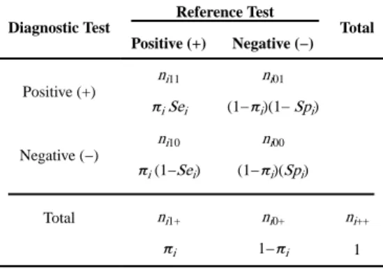
Here, we consider a trivariate GLMM based on the parameterization of πi, Sei and Spi,
where πi is the disease prevalence in the ith study. The first level of this model assumes
binomial distributions:
(7)
The parameters are modeled via link functions: g(πi) = ε0 + εi, g (Sei) = μ0 + μi and g (Spi)
=ν0 +νi. See Table 2 a two by two table accounting for disease prevalence.
To consider heterogeneity and potential correlations of the 3 parameters, εi, μi and νi are
assumed to be random effects with trivariate normal distribution:
A
uthor Man
uscr
ipt
A
uthor Man
uscr
ipt
A
uthor Man
uscr
ipt
A
uthor Man
uscr
The parameters capture the between-study variance of the disease prevalence, sensitivity and specificity while ρεμ, ρεν, ρμν represent correlations.
Standard software such as SAS NLMIXED can maximize this likelihood. To avoid including unnecessary parameters, model selection criteria such as AIC can be used. The medians are
derived as π̂M =g−1(ε̂0), and . In this model, covariates can be
incorporated for sensitivities, specificities and disease prevalence as was done for the bivariate GLMM.
3. Statistical methods when the reference test is not a gold standard
Limited meta-analysis tools are available when the reference test is imperfect. Walter et al.
discussed the latent class model for a meta-analysis of two diagnostic tests.18 Sadatsafavi et
al. presented a latent class random effects model.20 However, beyond prevalence, only one
of the sensitivity and specificity can be implemented as a random effect. Dendukuri et al. presented a Bayesian approach, which is an extension of the hierarchical summary ROC
model, to adjust for different reference standards.21 We describe the latent class random
effects model by Chu et al. using random effects to allow variation and correlation in
sensitivity, specificity and prevalence between studies.19
Let (SeBi, SpBi) be the pair of diagnostic accuracy parameters for the reference test while
(SeAi, SpAi) be the pair for the diagnostic test of interest. To construct the 2 by 2 table (Table
3) for such studies, both the above pairs of statistics and the disease prevalence are needed.
The four counts in Table 3 follow a multinomial distribution, with the log-likelihood being:
(8)
Chu et al. used random effects to model between and within study heterogeneity and
potential correlations.19 We write this model in a form suitable for a general link function:
A
uthor Man
uscr
ipt
A
uthor Man
uscr
ipt
A
uthor Man
uscr
ipt
A
uthor Man
uscr
where random effects follow a multivariate normal distribution: (εi, μAi, νAi, μBi, νBi)′ ~ N
(0, Σ) with variance-covariance matrix
.
Median estimates of prevalence, sensitivities and specificities can be constructed as π̂M =
g−1(ε̂0), and .
Variance and correlation parameter estimates can be derived from Σ̂. Covariates Zi can be
adjusted by linear regressions for the mean vectors, for instance g(πi) =ε0 +εi +γZi.
This latent class random effects model fills a gap in the existing models for meta-analysis with imperfect reference tests. This model can be used to evaluate the performance of both the diagnostic test of interest and the reference test while retaining all the advantages of the GLMMs. A limitation applies when fitting this model by SAS NLMIXED. One may encounter convergence problems because of the limited number of studies and relatively large number of parameters. Possible simplification of model assumptions may include letting disease prevalence be independent of sensitivities and specificities. Also, to avoid including unnecessary random effects whose variance approaches zero, one can apply a forward selection based on AIC. We will illustrate this process in Section 4.2 with an example.
4. Case Study
4.1 A meta-analysis of rotator cuff tears diagnosis using ultra-sound
4.1.1 Study background—We demonstrate an application of the methods in Section 2 using data on ultra-sound diagnosis of rotator cuff tears. Rotator cuff tears are a common reason for shoulder pain, which is the third most common musculoskeletal complaint. The incidence of partial rotator cuff tears is reported to be 13% to 32% in cadaveric studies, yet
much of this incidence goes undiagnosed.35 Among the diagnostic tests for this disease,
ultrasound is non-invasive and less expensive. However, it has lower sensitivity and
specificity in detecting the disease than MRI or arthroscopic evaluation.36 We will
re-analyze the data from a meta-analysis of 30 studies of diagnostic accuracy of ultrasound for
rotator cuff tears in adults, performed by Smith et al.37 The studies compared the accuracy
of ultrasound with either arthroscopic or open surgical findings as a gold standard test. The data is presented in Appendix A1. Figure 1 and 2 present the forest plots of sensitivity and specificity, respectively. In the rest of this section, we explore this example using the models discussed in Section 2. The corresponding SAS code can be found in Appendix B1-B6.
4.1.2 Summary ROC method—Applying the summary ROC method, we analyze the data first by unweighted least squares, then by weighted least squares. The un-weighted
method gives estimates â =3.39, b̂ =0.131 and AUC=0.911. The AUC can be interpreted as a
likelihood of 91.11% that a randomly selected diseased subject will receive a more
A
uthor Man
uscr
ipt
A
uthor Man
uscr
ipt
A
uthor Man
uscr
ipt
A
uthor Man
uscr
suspicious rating than a non-diseased subject. The weighted method give estimates âw
=3.573, b̂w =0.400 and AUCw=0.910. To build the summary ROC curve, we plug in â and b̂
(âw and b̂w) into equation (1) then plot Se against 1–Sp. The summary ROC curves are
presented in Figure 3.
4.1.3 Bivariate LMM—To fit the bivariate linear mixed model, we use the SAS procedure MIXED. The bivariate LMM method can provide summary estimates of sensitivity and
specificity other than the summary ROC curve. Parameter estimates are: μ̂ =1.351, ν̂ =
1.853, , σ̂μν = −0.116. The sensitivity and specificity are estimated as
and . Correlation estimate is ρ̂ = −0.18. The standard errors (SE)
can be calculated by delta method: and . Plugging in the
estimates into the equation (3), one can draw the summary ROC curve as presented in Figure 3. This model gives an AUC of 0.858. With the estimated medians, standard errors and correlation coefficients, one can draw confidence and prediction regions around the median estimates. Compared with the summary ROC method, the Bivariate LMM can provide summary estimates of overall sensitivity and specificity and their confidence regions. It may be more intuitive for investigators to compare different diagnostic tests.
4.1.4 Hierarchical summary ROC model—The hierarchical summary ROC model is
fitted using the SAS procedure NLMIXED. Estimates of the parameters are: θ̂0 = −0.738, σ̂θ
= 0.708, α̂0 = 3.887, σ̂α = 1.045 and β̂ = −0.522. The median sensitivity and specificity are
with SE 0.042 and with SE 0.021. To draw the summary ROC
curve, plug in the estimates into the expected logit sensitivity given specificity as in equation (5), then transform to ROC space, as presented in Figure 3. The AUC is 0.908.
4.1.5 Bivariate GLMM method—The bivariate GLMM models are fitted using the SAS procedure NLMIXED under three link functions: logit, probit and complementary log-log. The ‘estimate’ statements in the NLMIXED procedure can transform the parameter
estimates to median sensitivity and specificity and carry out the estimation of standard errors via delta method. Table 4 reports summary indexes with standard errors. When dependence is assumed in the model, the three links give comparable summary estimates. The logit link provides the smallest AIC (214.8), and thus selected as the best fitted model. However, the negative correlation estimate has a large standard error. In fact, if one fit a logit link GLMM assuming independence, the AIC (213.5) is slightly smaller than the correlated model. This example does not strongly support correlation between sensitivity and specificity.
To summarize estimates from bivariate models, we compare the bivariate LMM method, hierarchical summary ROC model and GLMM model using logit link. The summary ROC curves and confidence and prediction ellipses of these models are presented in Figure 3. Hierarchical summary ROC and GLMM models achieve same sensitivity and specificity median estimates and standard errors, which agrees with the argument by Harbord et al. that
the two models are the same with different parameterizations.6 The bivariate LMM model
has lower estimates of sensitivity and specificity. The differences may be due to the continuity correction applied in bivariate LMM and the some degrees of approximation
A
uthor Man
uscr
ipt
A
uthor Man
uscr
ipt
A
uthor Man
uscr
ipt
A
uthor Man
uscr
involved in the MIXED procedure when study size is small.6 A simulation study from Chu and Cole demonstrated that the GLMM method provides unbiased estimates while the
bivariate LMM model has biased estimates of SeM, SpM and ρ.12
4.1.6 Trivariate GLMM—When the prevalence of disease is involved as in a trivariate model, case-control studies need to be excluded. All our studies included satisfy the 1st
criterion in the QUADAS checklist which requires random selection of the sample.37
To successfully capture possible correlations without including unnecessary correlations, we fit models with all possible correlation combinations. The parameters and desired estimates, AIC and log-likelihoods are summarized in Table 5. The best model with the smallest AIC of 2653.8 is model I with no correlations (boldfaced estimates in Table 5). This suggests no correlations among disease prevalence, sensitivity and specificity in this example. This conclusion agrees with the bivariate GLMM and the estimated median sensitivity and specificity are similar as the estimates from bivariate GLMM method using logit link in Section 4.1.5. This example shows that, when the prevalence is weakly correlated with sensitivity and specificity, the bivariate GLMM gives very similar estimates to that from the trivariate GLMM.
4.2 A meta-analysis of cervical cancer diagnosis using Pap smears test
In this section, we re-visit the example used by Walter et al. 18 and apply the latent class
random effects models. The data is collected from a meta-analysis of Papanicolau (Pap) smears test accuracy by Fahey et al. The Pap smear is a quick, noninvasive and relatively
inexpensive test for cervical cancer.38 Fahey’s analysis consists of 59 cross-sectional studies
using Pap smears as the diagnostic test and histology as the gold standard. However, Walter’s model argued that the histology test has sensitivity of 0.97 and specificity of 0.62,
revealing lack of a perfect gold standard.18 Hence we will treat histology as an imperfect
reference test then fit the data by the latent class random effects models in Section 3. The data is listed in Appendix A2 and corresponding SAS code is included in Appendix B7.
When fitting the model using the SAS procedure NLMIXED, convergence problems appeared as more random effects were added. Thus we assume prevalence to be independent of sensitivities and specificities for ease of fitting and apply a forward-selection procedure to select random effects. We begin with a fixed effects model, and add random effects
sequentially. The process of selection is outlined in Table 6. The final model obtained is IVe, in which random effects are considered for the disease prevalence, Pap smear test sensitivity and specificity and the specificity of the histology test. The parameter estimates of the best fitted models at each step are provided in Table 7.
After adjustment for possible variation and correlations by random effects in our method, the final model IVe shows a low sensitivity for the Pap smears of 0.655 (SE=0.042) and a specificity of 0.835 (SE=0.032). However, the histology test outperforms the Pap smears with sensitivity of 0.903 (SE=0.013) and specificity of 0.989 (SE=0.014). Moreover, our estimates of the histology test differ from the estimates in Walter’s, suggesting a somewhat
different interpretation in practice.18
A
uthor Man
uscr
ipt
A
uthor Man
uscr
ipt
A
uthor Man
uscr
ipt
A
uthor Man
uscr
5. Discussion
In this paper, we discussed methods for evaluating the performance of diagnostic tests for situations when the reference test can be considered a gold standard, as well as situations when it is error-prone. Under the scenario with a gold standard, we reviewed the traditional summary ROC method, bivariate LMM and the hierarchical summary ROC model. Then we focused on the random effect GLMM, because it has several advantages over the simpler methods. We showed how the bivariate GLMM can be fitted using a variety of link functions including logit, probit and complementary log-log, and extended the approach to a trivariate GLMM to jointly model prevalence, sensitivity and specificity. Under the situation with no
gold standard, we built upon the latent class model proposed by Walter et al.18 by adding
random effects to quantify possible correlation and variation following the methods by Chu
et al..19 We worked through two empirical examples to illustrate the application of our
models. We used the SAS procedures MIXED and NLMIXED to fit all models, and provide SAS code with detailed explanation in the Appendix. The SAS macro METADAS may assist in automating the fitting of bivariate and hierarchical summary ROC models for
meta-analysis of diagnostic tests.39
Several extensive simulation studies have been conducted in the literature to compare
different methods. Hamza et al.40 studied the univariate exact binomial likelihood approach
against the univariate approximate normal likelihood approach in different simulation settings. The size of meta-analysis varied from 10 to 100 studies and the true median sensitivity values ranged from 0.6 to 0.93. Overall the simulations showed that the exact likelihood approach performs superior than the approximate approach in terms of bias and
coverage probabilities. Riley et al.41 compared the bivariate random-effects meta-analysis
dealing with dependence between two outcomes to the univariate random-effects meta-analysis. Simulation studies showed that the bivariate approach has smaller mean-square
error and is recommended over the univariate approach. Chu et al.12 conducted simulations
to study the bivariate GLMM and the BLMM approaches. Size of meta-analysis varied from 25 to 250, and Se/Sp was either relatively low (0.7/0.8) or relatively high (0.9/0.95). The bivariate GLMM was shown to yield unbiased estimates of Se, Sp and their correlation,
while the BLMM gave biased results. Another paper of Chu et al.31 conducted simulations
to compare different links used in bivariate GLMM with 40 meta-studies, 200 subjects in each study and median Se/Sp as 0.8/0.9. It suggested that the AUC and median Se/Sp estimates are relatively robust to the choice of link functions. The trivariate GLMM and
bivariate GLMM were compared in Chu et al.17 under different correlation assumptions. The
results suggested that misspecification resulting from AIC-based model selection is
reasonably low in studied settings. When the reference test is imperfect, Chu et al.19 used
different selection criteria DIC, AIC and BIC on selecting the appropriate random effects. The simulation results recommended including random effects because omitting important variability can cause inflated variance and decreased coverage.
Among the models presented, the summary ROC approach is simple and widely used. However, it is limited as it does not assess the within- and between-study variations and possible correlations between Se and Sp. The bivariate LMM improves over the summary ROC approach by assuming random effects to explain both within- and between-study
A
uthor Man
uscr
ipt
A
uthor Man
uscr
ipt
A
uthor Man
uscr
ipt
A
uthor Man
uscr
variations and possible correlations. The bivariate LMM can provide inferences both in terms of summary ROC curves and summary statistics of overall test performance. However, it has limitations due to the use of a continuity correction and a normal approximation. The GLMMs do not have the limitations of the above models because they assume exact binomial distributions. The bivariate GLMM, which is essentially the same as the hierarchical summary ROC model in certain situations, is recommended when research interests focus on sensitivity and specificity and there’s strong suggestion of independence with disease prevalence. The trivariate GLMM will be most appropriate when there’s interest in estimating PPV or NPV, because estimation of disease prevalence is required and correlation among prevalence and Se, Sp should not be ignored. Besides, the trivariate GLMM is most reliable when most of the studies are cohorts. When the reference test is not a gold standard, the latent class random effects model should be used to avoid biased estimates.
A limitation related to the GLMMs is that the meta-analysis reported often includes a mixture of case-control and cohort studies designs. Thus using either the bivariate or the trivariate GLMM for all the studies can lead to problems. Another issue arises when fitting the trivariate GLMM and the latent class random effects models in the SAS procedure NLMIXED. The more random effects included, the longer it takes to converge. Under such situations, one can first get raw estimates of the desired parameters by fitting the data in models with fewer random effects. The raw estimates can then be used as starting values to improve convergence in a more complex model. For the latent class random effects model, one may need to apply simpler assumptions for ease of fitting. For instance, our example assumes independence between prevalence and the paired indices. However, as discussed, dependence between the indices may be expected.
In the example of rotator cuff tears, we excluded seven studies having the partial verification problem to avoid biased results, though these studies might still be able to contribute to our analysis. To the best of our knowledge, multivariate methods to correct publication bias in a meta-analysis of diagnostic test settings still await for further development. A recent Bayesian approach to correct such bias by de Groot et al. may be applied to diagnostic tests
with nominal outcomes.42 In summary, sensitivity analysis methods for meta-analysis of
diagnostic tests investigating the impact of publication bias through a selection or pattern mixture model framework are yet to be developed.
Acknowledgments
This research was supported in part by the U.S. Department of Health and Human Services Agency for Healthcare Research and Quality Grant R03HS020666, P01CA142538 and P30CA77598 from the U.S. National Cancer Institute, and R21AI103012 from the U.S. National Institute of Allergy and Infectious Diseases.
References
1. Zhou, XH.; Obuchowski, NA.; McClish, DK. Statistical methods in diagnostic medicine. New York: John Wiley & Sons; 2002.
2. Pepe, MS. The statistical evaluation of medical tests for classification and prediction. Oxford: Oxford University Press; 2003.
A
uthor Man
uscr
ipt
A
uthor Man
uscr
ipt
A
uthor Man
uscr
ipt
A
uthor Man
uscr
3. Rutter CA, Gatsonis CA. A hierarchical regression approach to meta-analysis of diagnostic test accuracy evaluations. Statistics in Medicine. 2001; 20:2865–84. [PubMed: 11568945] 4. Song F, Khan KS, Dinnes J, Sutton AJ. Asymmetric funnel plots and publication bias in
meta-analyses of diagnostic accuracy. International Journal of Epidemiology. 2002; 31:88–95. [PubMed: 11914301]
5. van Houwelingen HC. Advanced methods in analysis: multivariate approach and meta-regression. Statistics in Medicine. 2002; 21:589–624. [PubMed: 11836738]
6. Harbord RM, Deeks JJ, Egger M, Whiting P, Sterne JAC. A unification of models for meta-analysis of diagnostic accuracy studies. Biostatistics. 2007; 8:239–51. [PubMed: 16698768]
7. Macaskill P. Empirical Bayes estimates generated in a hierarchical summary ROC analysis agreed closely with those of a full Bayesian analysis. Journal of Clinical Epidemiology. 2004; 57:925–32. [PubMed: 15504635]
8. Mallett S, Deeks JJ, Halligan S, Hopewell S, Cornelius V, Altman DG. Systematic reviews of diagnostic tests in cancer: review of methods and reporting. BMJ. 2006; 333:413. [PubMed: 16849365]
9. Zwinderman AH, Bossuyt PM. We should not pool diagnostic likelihood ratios in systematic reviews. Statistics in Medicine. 2008; 27:687–97. [PubMed: 17611957]
10. Arends LR, Hamza TH, van Houwelingen JC, Heijenbrok-Kal MH, Hunink MGM, Stijnen T. Bivariate Random Effects Meta-Analysis of ROC Curves. Medical Decision Making. 2008; 28:621–38. [PubMed: 18591542]
11. Reitsma JB. Bivariate analysis of sensitivity and specificity produces informative summary measures in diagnostic reviews. Journal of Clinical Epidemiology. 2005; 58:982–90. [PubMed: 16168343]
12. Chu H, Cole SR. Bivariate meta-analysis of sensitivity and specificity with sparse data: a generalized linear mixed model approach. Journal of clinical epidemiology. 2006; 59:1331–2. [PubMed: 17098577]
13. Chu H, Guo H. Letter to the editor: a unification of models for meta-analysis of diagnostic accuracy studies. Biostatistics. 2009; 10:201–3. [PubMed: 19039031]
14. Riley R, Abrams K, Sutton A, Lambert P, Thompson J. Bivariate random-effects meta-analysis and the estimation of between-study correlation. BMC Medical Research Methodology. 2007; 7:3. [PubMed: 17222330]
15. Riley RD, Abrams KR, Lambert PC, Sutton AJ, Thompson JR. An evaluation of bivariate random-effects meta-analysis for the joint synthesis of two correlated outcomes. Statistics in Medicine. 2007; 26:78–97. [PubMed: 16526010]
16. Hamza TH, van Houwelingen HC, Stijnen T. The binomial distribution of meta-analysis was preferred to model within-study variability. Journal of Clinical Epidemiology. 2008; 61:41–51. [PubMed: 18083461]
17. Chu H, Nie L, Cole SR, Poole C. Meta-analysis of diagnostic accuracy studies accounting for disease prevalence: Alternative parameterizations and model selection. Statistics in Medicine. 2009; 28:2384–99. [PubMed: 19499551]
18. Walter SD, Irwig L, Glasziou PP. Meta-analysis of diagnostic tests with imperfect reference standards. Journal of Clinical Epidemiology. 1999; 52:943–51. [PubMed: 10513757]
19. Chu H, Chen SN, Louis TA. Random Effects Models in a Meta-Analysis of the Accuracy of Two Diagnostic Tests Without a Gold Standard. Journal of the American Statistical Association. 2009; 104:512–23. [PubMed: 19562044]
20. Sadatsafavi M, Shahidi N, Marra F, et al. A statistical method was used for the meta-analysis of tests for latent TB in the absence of a gold standard, combining random-effect and latent-class methods to estimate test accuracy. JClinEpidemiol. 2010; 63:257–69.
21. Dendukuri N, Schiller I, Joseph L, Pai M. Bayesian Meta-Analysis of the Accuracy of a Test for Tuberculous Pleuritis in the Absence of a Gold Standard Reference. Biometrics. 2012
22. Moses LE, Shapiro D, Littenberg B. Combining Independent Studies of A Diagnostic-Test Into A Summary Roc Curve - Data-Analytic Approaches and Some Additional Considerations. Statistics in Medicine. 1993; 12:1293–316. [PubMed: 8210827]
A
uthor Man
uscr
ipt
A
uthor Man
uscr
ipt
A
uthor Man
uscr
ipt
A
uthor Man
uscr
23. Walter SD. Properties of the summary receiver operating characteristic (SROC) curve for diagnostic test data. Statistics in Medicine. 2002; 21:1237–56. [PubMed: 12111876]
24. Walter SD. The partial area under the summary ROC curve. Statistics in Medicine. 2005; 24:2025– 40. [PubMed: 15900606]
25. Sutton AJ, Cooper NJ, Goodacre S, Stevenson M. Integration of Meta-analysis and Economic Decision Modeling for Evaluating Diagnostic Tests. Medical Decision Making. 2008; 28:650–67. [PubMed: 18753686]
26. Irwig L, Tosteson ANA, Gatsonis C, et al. Guidelines for Meta-analyses Evaluating Diagnostic Tests. Annals of Internal Medicine. 1994; 120:667–76. [PubMed: 8135452]
27. Deeks JJ. Systematic reviews in health care: systematic reviews of evaluations of diagnostic and screening tests. British Medical Journal. 2001; 323:157–62. [PubMed: 11463691]
28. Sweeting MJ, Sutton AJ, Lambert PC. What to add to nothing? Use and avoidance of continuity corrections in meta-analysis of sparse data. Stat Med. 2004; 23:1351–75. [PubMed: 15116347] 29. Starmer CF, Grizzle JE, Sen PK. Some reasons for not using the Yates continuity corrections in meta-analysis of sparse data. Journal of the American Statistical Association. 1974; 69:376–8. 30. Tosteson AN, Begg CB. A general regression methodology for ROC curve estimation.
MedDecisMaking. 1988; 8:204–15.
31. Chu H, Guo H, Zhou Y. Bivariate Random Effects Meta-Analysis of Diagnostic Studies Using Generalized Linear Mixed Models. Medical Decision Making. 2010; 30:499–508. [PubMed: 19959794]
32. Ransohoff DF, Feinstein AR. Problems of spectrum and bias in evaluating the efficacy of diagnostic tests. NEnglJMed. 1978; 299:926–30.
33. Brenner H, Gefeller O. Variation of sensitivity, specificity, likelihood ratios and predictive values with disease prevalence. Statistics in Medicine. 1997; 16:981–91. [PubMed: 9160493]
34. Li J, Fine JP. Assessing the dependence of sensitivity and specificity on prevalence in meta-analysis. Biostatistics. 2011
35. Shin KM. Partial-thickness rotator cuff tears. Korean J Pain. 2011; 24:69–73. [PubMed: 21716613] 36. Singisetti K. Shoulder ultrasonography versus arthroscopy for the detection of rotator cuff tears:
analysis of errors. J Orthop Surg (Hong Kong). 2011 Apr; 19(1):76–9. [PubMed: 21519083] 37. Smith TO. Diagnostic accuracy of ultrasound for rotator cuff tears in adults: A systematic review
and meta-analysis. Clinical Radiology. 2011 Jul 5.
38. Fahey MT, Irwig L, Macaskill P. Meta-analysis of Pap test accuracy. American Journal of Epidemiology. 1995; 141:680–9. [PubMed: 7702044]
39. Takwoingi, Y.; Deeks, JJ. METADAS: an SAS macro for meta-analysis of diagnostic accuracy studies. 2011.
40. Hamza TH, van Houwelingen HC, Stijnen T. The binomial distribution of meta-analysis was preferred to model within-study variability. Journal of clinical epidemiology. 2008; 61:41–51. [PubMed: 18083461]
41. Riley RD, Thompson JR, Abrams KR. An alternative model for bivariate random-effects meta-analysis when the within-study correlations are unknown. Biostatistics (Oxford, England). 2008; 9:172–86.
42. de Groot JA, Dendukuri N, Janssen KJ, et al. Adjusting for partial verification or workup bias in meta-analyses of diagnostic accuracy studies. American Journal of Epidemiology. 2012; 175:847– 53. [PubMed: 22422923]
Appendix A. Data for case studies
Appendix A1
Partial rotator cuff tears meta-analysis data
study year True positive False positive False negative True negative
Al-Shawi 2008 65 12 1 65
A
uthor Man
uscr
ipt
A
uthor Man
uscr
ipt
A
uthor Man
uscr
ipt
A
uthor Man
uscr
study year True positive False positive False negative True negative
Alasaarela 1998 1 0 0 19
Brenneke and Morgan 1992 11 8 14 45
Cullen 2007 11 2 3 21
Ferrari 2002 8 1 10 25
Friedman 1993 2 0 2 0
Hedtmann and Fett 1995 121 0 12 0
Iannotti 2005 26 7 2 16
Kang 2009 2 5 2 5
Kayser 2005 41 16 11 171
Labanauskaite 2002 11 3 2 9
Milosavljevic 2005 17 0 7 6
Naqvi 2009 4 2 0 11
Read et al 1998 6 1 7 28
Roberts et al 2001 5 0 2 7
Rutten et al 2010 8 12 0 24
Takagishi 1996 10 7 10 57
Teefey 2000 10 3 5 17
Teefey 2005 13 4 2 52
van Holsbeeck et al 1995 14 3 1 47
Vlychou et al 2009 44 2 3 7
Wiener and Seitz 1993 64 4 3 71
Yen et al 2004 9 1 1 9
Appendix A2
Pap smear test meta-analysis data
Study Type* ni11 ni10 ni00 ni01
Alloub et al SC 8 23 84 3
Alons-van Kordelaar and Boon SC 31 43 14 3
Anderson et al SC 70 121 25 12
Anderson et al FU 65 6 6 10
Anderson et al FU 20 19 4 3
Andrews et al FU 35 20 156 92
August FU 39 111 271 7
Bigrigg et al SC 567 140 157 117
Bolger and Lewis SC 26 12 18 37
Byme et al FU 38 17 37 28
Chomet SC 45 15 48 35
Engineer and Misra SC 71 10 306 87
Fletcher et al FU 4 36 5 0
Frisch et al SC 2 3 21 2
Giles et al SC 5 3 182 9
A
uthor Man
uscr
ipt
A
uthor Man
uscr
ipt
A
uthor Man
uscr
ipt
A
uthor Man
uscr
Study Type* ni11 ni10 ni00 ni01
Giles et al FU 38 7 62 21
Gunderson et al SC 4 16 31 2
Haddad et al SC 87 12 9 13
Hellberg et al SC 15 65 15 3
Helmerhorst et al FU 41 61 29 1
Hirschowitz et al FU 76 11 12 12
Jones DED et al FU 10 48 174 4
Jones MH et al FU 28 28 77 11
Kashimura et al SC 3 5 1 0
Kealy FU 79 13 182 26
Koonlng-1 et al FU 61 27 35 20
Koonlng-2 et al FU 62 16 49 20
Kwikkel et al FU 284 68 68 31
Lozowski et al FU 66 20 44 25
Maggi et al FU 40 12 47 43
Morrison EAB et al FU 11 1 2 1
Morrison BW et al SC 23 10 44 50
Nyirjesy SC 65 42 13 13
Okagaki and Zelterman SC 1270 263 1085 927
Oyer and Hanjanl FU 223 74 83 22
Parker SC 154 20 237 30
Pearlstone et al FU 6 12 81 2
Ramlrez et al SC 7 3 4 4
Reld et al SC 12 11 60 5
Robertson et al FU 348 212 103 41
Schauberger et al SC 8 11 34 4
Shaw FU 12 6 0 2
Singh et al FU 95 2 1 9
Skehan et al FU 40 20 19 18
Smith et al FU 71 20 18 13
Soost et al SC 1205 454 241 186
Soutter-1 et al SC 5 52 27 20
Soutter-2 et al SC 35 12 12 9
Spitzer et al FU 10 5 32 31
Stafi SC 3 3 15 5
Syrjanen et al FU 118 44 183 40
Szarewski SC 13 82 17 3
Tait et al SC 38 13 62 14
Tawa et al SC 14 67 291 25
Tay et al FU 12 6 12 14
Upadhyay et al SC 238 2 16 52
Walker et al FU 111 20 39 44
A
uthor Man
uscr
ipt
A
uthor Man
uscr
ipt
A
uthor Man
uscr
ipt
A
uthor Man
uscr
Study Type* ni11 ni10 ni00 ni01
Wetrich FU 491 250 702 164
Wheelock and Kamlnlski FU 49 39 31 16
*
type of the study denotes the usage of the test clinically, SC as screening and FU as follow up.
Appendix B. SAS codes for fitting models
B1. Unweighted summary ROC
data partial1; | /*‘tp’ stands for true
positive, ‘fp’ for
set partial; | false positive, ‘fn’ for
false negative, ‘tn’
if tp = 0 or fp = 0 or fn = 0 or tn = 0 then do; | for true
negative */
tp=tp+0.5; fp=fp+0.5; fn=fn+ 0.5; tn=tn+ 0.5; | /*continuity
correction on zero cells*/
n0=n0+1; n1=n1+1; end;
se= tp/n1; sp=tn/n0; | /*calculate Se and Sp
for each study*/
logitse = log(se/(1-se)); var logitse=1/(se*(1-se)*n1); | /* logit(Se) and
logit(Sp) and their
logitsp = log(sp/(1-sp)); var logitsp=1/(sp*(1 -sp)*n0); | variances*/
D=logitse+logitsp; S=logitse-logitsp; | /* D and S*/
proc reg data=partial1; model D=S; run; | /*fit linear
regression model D=a+bS*/
B2. Weighted summary ROC
data partial2; set partial1;
w=1/(1/tp+1/fp+1/tn+1/fn); | /*calculate the weight
for each study*/
proc reg data=partial2; model D=S; weight w; run; | /*fit weighted
regression using the created
| weights*/
B3. SAS MIXED procedure to fit bivariate LMM
data partial3; set partial1; id= n_; | /* make each study have two
observations, one for
dis=1; non dis=0; logit=logitse; | sensitivity, the other for
A
uthor Man
uscr
ipt
A
uthor Man
uscr
ipt
A
uthor Man
uscr
ipt
A
uthor Man
uscr
specificity.*/
var logit=var logitse; rec+ 1; output;
dis=0; non dis=1; logit=logitsp;
var logit=var_logitsp; rec+1 ; output; run;
data cov; | /* build the data containing
variable ‘est’ with 3 starting
if n eq 1 then do; | values for the covariance
parameters of the random effects
est=0; output; est=0; output; est=0 ; output; | and 60 within study arm
variances.*/
end;
set partial3; est = var_logit; output;
keep est; run;
proc mixed data=partial3 method=reml cl; | /*choose the residual
(restricted) method(reml), ‘cl’ asks
class id; | for confidence limits for
covariance parameter estimates.*/
model logit= dis non_dis / noint s cl covb | /*indicator variables ‘dis’
and ‘non_dis’ are explanatory
df=1000, 1000; | variables for logit(Se) and
logit(Sp). ‘covb’ asks for
| covariance matrix of fixed effects
parameters. Large ‘df”
| approximate a t distribution to a
normal distribution.*/
random dis non_dis / subject=id type=un s; | /* random effects
corresponds to disease and non_disease
| status. An unstructured working
covariance structure is
| stated to assume possible
correlation of ‘dis’ and ‘non_dis’
| within the same study.*/
repeated / group=rec; | /* ‘group=rec’ statement
specifies the with-in study-arm
| variance in each study.*/
parms / parmsdata=cov hold=4 to 63 ; | /*‘parmsdata’ option reads in
variable ‘est’ from the cov
run; | data. 60 within study-arm variances
are kept constant.*/
B4. SAS NLMIXED procedure to fit the hierarchical summary ROC Model
data partial4; set partial; id= n ; | /* make each
study has two records */
A
uthor Man
uscr
ipt
A
uthor Man
uscr
ipt
A
uthor Man
uscr
ipt
A
uthor Man
uscr
dis=0.5; ny=tp; n=n1; se=1; output; | /*code ‘dis’ as
0.5 and ‘se’=1 for disease
dis=-0.5; ny=tn; n=n0; se=0 ; output; | patients, ‘dis’
as -0.5 and ‘se’=0 for
non-keep id ny n dis se; run; | disease subjects*/
proc nlmixed data=partial4;
parms theta=-1 alpha=4 beta=-0.6 sigtheta=0.7 sigalpha=1.7; | /* assign
starting values for parameters.*/
logitp=2*dis*((theta+ut)+(alpha+ua)*dis)*exp(-beta*dis); | /* code
‘logitp’ as logit(Se) and logit(Sp)
| */
p=exp(logitp)/(1+exp(logitp)); | /*logit transform
is applied to the
| probabilities*/
model ny~binomial(n,p); | /* number of tp and
tn are Bin(n, p)
| distributed */
random ut ua ~ | /* ‘ut’ and ‘ua’ are
random effects
normal([0,0],[exp(2*sigtheta),0,exp(2*sigalpha)]) subject=id; | clustered
within study. Independence is
| assumed between random
effects.
| Exponential formed
variance is to ensure
estimate "se" 1/(1+exp(-((theta+0.5*alpha)*exp(-0.5*beta)))); |
positivity.*/
estimate "sp" 1/(1+exp((theta-0.5*alpha)*exp( 0.5*beta))); | /*use
estimate statement to get
estimate "sigtheta" exp(sigtheta); estimate "sigalpha" | estimates
of desired indices with standard
exp(sigalpha); run; | errors. */
B5. SAS NLMIXED procedure to fit bivariate GLMM with logit link
proc nlmixed data=partial4 fd cov corr df=1000 gtol=1e-11; | /* ‘fd’
specifies that all derivatives be
parms mu0=1.5 nu0=-2.2 fz= 0.23 sigse=0.37 sigsp=-0.26; | computed using
finite difference
| approximations. /
rho= (exp(2*fz)-1)/(1+exp(2*fz)); | /* use fisher’s z
transformation instead of
| the correlation
coefficient ρ directly to
A
uthor Man
uscr
ipt
A
uthor Man
uscr
ipt
A
uthor Man
uscr
ipt
A
uthor Man
uscr
if Se=1 then beta=mu0+mu; if Se=0 then beta=nu0+nv; | ensure –1 ≤ ρ 1*/
pred=exp(beta)/(1+exp(beta));
model ny~binomial(n, pred); | /* ‘tp’ and ‘tn’
are binomially distributed
| condition on random
effects ‘mu’ and
| ‘nv’.*/
random mu nv ~ normal([0, 0 ], | /*random effects
‘mu’ and ‘nv’ are
[exp(2*sigse), rho*exp(sigse)*exp(sigsp), | bivariate
normally distributed; ‘subject=id’
exp(2*sigsp)]) subject=id; | indicates possible
correlation of random
estimate "Se" exp(mu0)/(1+exp(mu0)); | effects within a
study*/
estimate "Sp" exp(nu0)/(1+exp(nu0)); run;
B6. SAS NLMIXED procedure to fit trivariate GLMM
proc nlmixed data=partial fd df=1000 gtol=1e-10; | /* model I is
the best fitted model with
parms mu0=0 nv0=3 eta0=-1 sigse=0 sigsp=0 sigpi=-1 ; | smallest AIC*/
logitsei = mu0 + mu; logitspi = nv0 + nv;
logitpi = eta0 + eta; | /*model
prevalence (‘pi’) together with
Sei= 1 /(1+exp(-logitsei)); Spi=1/(1+exp(-logitspi)); | Se and Sp*/
pi=1 /( 1+exp(-logitpi));
logL= tp * (log(pi) + log(Sei )) + fp * (log(1-pi) + log( 1-Spi)) |
/*log-likelihood for trivariate model*/
+ fn * (log(pi) + log(1-Sei)) + tn * (log(1-pi) + log(Spi )); | /
*specify general log-likelihood
model Y ~ general(logL); | function. Any
variable can be used as the
| dependent variable in
this situation.*/
random mu nv eta~normal([0, 0, 0], | /*‘mu’, ‘nv’
and ‘eta’ are the random
[exp(2*sigse), | effects
corresponding to Se, Sp and
0, exp(2*sigsp), | prevalence.
Possible correlation could
0, 0, exp(2*sigpi)]) subject=id; | exist within
studies. The best model is
estimate "sigse" exp(sigse); | achieved when
A
uthor Man
uscr
ipt
A
uthor Man
uscr
ipt
A
uthor Man
uscr
ipt
A
uthor Man
uscr
all the correlation
estimate "sigsp" exp(sigsp); | coefficients
among the random effects
estimate "sigpi" exp(sigpi); | ‘mu’, ‘nv’,
‘eta’ are zero.*/
estimate "Se" 1/(1+exp(-mu0));
estimate "Sp" 1/(1+exp(-nv0)); run;
B7. SAS NLMIXED procedure to fit the latent class random effect model IVe
for Pap Smears test
proc nlmixed data=walter1999 cov fd;
parms mua0=0.6 nva0=1.6 mub0=2 nvb0=4.5 eta0=0.6
sigpi=0.4 sigmua=0.3 signva=0.2 sigmub=0 fz2=-0.5; | /* five
parameters are
| modeled: ‘SeA’
and ‘SpA’ for
SeA=exp(mua0+mua)/(1+exp(mua0+mua)); | the Pap smear
test, ‘SeB’ and
SpA =exp(nva0+nva)/(1+exp(nva0+nva)); | ‘SpB’ for
the histology test
SeB=exp(mub0)/(1+exp(mub0)); | and ‘pi’ for
disease
SpB =exp(nvb0)/(1+exp(nvb0)); | prevalence*/
pi=exp(eta0+eta)/(1+exp(eta0+eta)); | /
*fisher’s z transformation;
| model V with
correlation only
rho2=(exp(2*fz2)-1)/(exp(2*fz2)+1); | between Se
and Sp of the Pap
| smear test*/
p11=pi*SeA*SeB+(1-pi)*(1-SpA)*(1 -SpB); | /*expected
probabilities in 2*2
p01=pi*SeA*(1-SeB)+(1-pi)*(1-SpA)*SpB; | table*/
p10=pi*(1-SeA)*SeB+(1-pi)*SpA*(1-SpB);
p00=pi*(1-SeA)*(1-SeB)+(1-pi)*SpA*SpB;
| /*log
likelihood*/
logl=n11*log(p11)+n01*log(p01)+n10*log(p10)+n00*log(p00);
model y ~ general(logl); | /*the best
model selected
random eta mua nva~normal([0,0,0],[exp(2 *sigpi), | evolves
four random effects.
A
uthor Man
uscr
ipt
A
uthor Man
uscr
ipt
A
uthor Man
uscr
ipt
A
uthor Man
uscr
0, exp(2*sigmua), | model IVe
assumes only
0, rho2*exp(sigmua)*exp(signva),exp(2*signva)]) |
correlation between ‘mua’ and
subject=id; | ‘nva’, i.e.
sensitivity and
estimate "SeA" exp(mua0)/(1+exp(mua0)) |
specificity of the Pap sme test
estimate "SpA" exp(nva0)/(1+exp(nva0)); | are
correlated.*/
estimate "pi" exp(eta0)/(1+exp(eta0));
estimate "rhomuanva" (exp(2*fz2)-1)/(exp(2*fz2)+1);
estimate "SeB" exp(mub0)/(1+exp(mub0));
estimate "SpB" exp(nvb0)/(1+exp(nvb0)); run;
A
uthor Man
uscr
ipt
A
uthor Man
uscr
ipt
A
uthor Man
uscr
ipt
A
uthor Man
uscr
Figure 1.
Forest plot for sensitivity in rotator cuff tears study
A
uthor Man
uscr
ipt
A
uthor Man
uscr
ipt
A
uthor Man
uscr
ipt
A
uthor Man
uscr
Figure 2.
Forest plot for specificity in rotator cuff tears study
A
uthor Man
uscr
ipt
A
uthor Man
uscr
ipt
A
uthor Man
uscr
ipt
A
uthor Man
uscr
Figure 3.
Summary median estimates and ROC curves from some of the introduced models. Panel A presents summary median Se and Sp estimates with confidence and predictive regions and summary ROC curve from the bivariate GLMM using logit link. Panel B presents summary median Se and Sp estimates with confidence and predictive regions and summary ROC curve from the BLMM and the summary ROC curve from the unweighted summary ROC method.
A
uthor Man
uscr
ipt
A
uthor Man
uscr
ipt
A
uthor Man
uscr
ipt
A
uthor Man
uscr
A
uthor Man
uscr
ipt
A
uthor Man
uscr
ipt
A
uthor Man
uscr
ipt
A
uthor Man
uscr
ipt
Table 1
2 by 2 table for ith study
Reference test
total
Positive (+) Negative (−)
Diagnostic Test
Positive (+) ni11 ni01
Negative (−) ni10 ni00
A
uthor Man
uscr
ipt
A
uthor Man
uscr
ipt
A
uthor Man
uscr
ipt
A
uthor Man
uscr
ipt
Table 2
2 by 2 table for ith study accounting for disease prevalence
Diagnostic Test
Reference Test
Total
Positive (+) Negative (−)
Positive (+)
ni11 ni01
πi Sei (1−πi)(1− Spi)
Negative (−)
ni10 ni00
πi (1−Sei) (1−πi)(Spi)
Total ni1+ ni0+ ni++