REAL-TIME SCHEDULING FOR GPUS WITH APPLICATIONS IN ADVANCED AUTOMOTIVE SYSTEMS
Glenn A. Elliott
A dissertation submitted to the faculty at the University of North Carolina at Chapel Hill in partial fulfillment of the requirements for the degree of Doctor of Philosophy in the Department of Computer Science.
Chapel Hill 2015
ABSTRACT
Glenn A. Elliott: Real-Time Scheduling for GPUs with Applications in Advanced Automotive Systems
(Under the direction of James H. Anderson)
Self-driving cars, once constrained to closed test tracks, are beginning to drive alongside human drivers on public roads. Loss of life or property may result if the computing systems of automated vehicles fail to respond to events at the right moment. We call such systems that must satisfy precise timing constraints “real-time systems.” Since the 1960s, researchers have developed algorithms and analytical techniques used in the development of real-time systems; however, this body of knowledge primarily applies to traditional CPU-based platforms. Unfortunately, traditional platforms cannot meet the computational requirements of self-driving cars without exceeding the power and cost constraints of commercially viable vehicles. We argue that modern graphics processing units, or GPUs, represent a feasible alternative, but new algorithms and analytical techniques must be developed in order to integrate these uniquely constrained processors into a real-time system.
The goal of the research presented in this dissertation is to discover and remedy the issues that prevent the use of GPUs in real-time systems. To overcome these issues, we design and implement a real-time multi-GPU scheduler, called GPUSync. GPUSync tightly controls access to a GPU’s computational and DMA processors, enabling simultaneous use despite potential limitations in GPU hardware. GPUSync enables tasks to migrate among GPUs, allowing new classes of real-time multi-GPU computing platforms. GPUSync employs heuristics to guide scheduling decisions to improve system efficiency without risking violations in real-time constraints. GPUSync may be paired with a wide variety of common real-time CPU schedulers. GPUSync supports closed-source GPU runtimes and drivers without loss in functionality.
execute computer vision programs similar to those found in automated vehicles, with and without GPUSync. Our results demonstrate that GPUSync greatly reduces jitter in video processing.
ACKNOWLEDGEMENTS
When I joined the computer science department at UNC, I largely believed that research as a graduate student was an independent affair: my success or failure depended entirely upon myself. I certainly would have failed had this been true. The completion of this dissertation is due in part to the knowledge, guidance, aid, and even love, from those I met and worked with during my time at Chapel Hill. I owe them all a great debt of gratitude.
First and foremost, I wish to thank my advisor, Jim Anderson, for taking a chance on a student who knew nothing of real-time systems and only thought “research on GPUs might be interesting.” On more than one occasion, Jim’s encouragement made it possible for me to complete a successful paper before a submission deadline when I had been ready to throw in the towel a day before. I would also like to thank the members of my committee, Sanjoy Baruah, Anselmo Lastra, Don Smith, Lars Nyland, and Shinpei Kato for their guidance in my research.
I also wish thank my wonderful colleagues of the Real-Time Systems Research Group at UNC. In particular, I am especially thankful for Björn Brandenburg and Bryan Ward. Björn’s tireless work on the LITMUSRToperating system, along with his techniques for real-time analysis, set the stage upon which I performed my work. The results of Bryan’s research on locking protocols (as well as Björn’s) figures heavily in the research presented herein. My work simply would not have been possible without the contributions of these two. I would also like to thank fellow LITMUSRTdevelopers Andrea Bastoni, Jonathan Herman, and Chris Kenna for helping me work through software bugs at any hour, as well as their willingness to offer advice during the implementation of the ideas behind my research. Additionally, I wish to thank my conference paper co-authors, Jeremy Erickson, Namhoon Kim, Cong Liu, and Kecheng Yang. I throughly enjoyed working with each of you. Finally, I would like to thank all of the other members of the real-time systems group, including Bipasa Chattopadhyay, Zhishan Guo, Hennadiy Leontyev, Haohan Li, and Mac Mollison.
Vlad Glavtchev, Mark Hairgrove, Chris Lamb, and Thierry Lepley for their guidance. I also wish to especially thank Elif Albuz and Michael Garland for giving me a free hand to explore.
I am also indebted to the staff of the UNC computer science department. I owe special thanks to Mike Stone for keeping my computing hardware going, Melissa Wood for keeping grant applications on track, and Jodie Turnbull for keeping the graduate school paperwork in order.
Finally, I wish to thank my parents and sisters for their love and support during the long years I was in North Carolina—thank you for not telling me that I was crazy for going back to school, even if you may have thought it, and even if you were right! I also want to thank Ryan and Leann McKenzie for their friendship; words cannot express how grateful I am. Lastly, I wish to thank Kim Kutz for her continued patience, love, and support, which sometimes took the form of fresh out-of-the-oven strawberry-rhubarb pie delivered to Sitterson Hall at one in the morning.
TABLE OF CONTENTS
LIST OF TABLES . . . xiv
LIST OF FIGURES . . . xvi
LIST OF ABBREVIATIONS . . . xx
Chapter 1: Introduction . . . 1
1.1 Real-Time Systems . . . 2
1.2 Graphics Processing Units . . . 3
1.3 Real-Time GPU Applications . . . 6
1.4 An Introduction to GPGPU Programming . . . 7
1.4.1 GPGPU Programming . . . 7
1.4.2 Real-Time GPU Scheduling . . . 9
1.4.3 Real-Time Multi-GPU Scheduling . . . 11
1.5 Thesis Statement . . . 11
1.6 Contributions . . . 12
1.6.1 A Flexible Real-Time Multi-GPU Scheduling Framework . . . 12
1.6.2 Techniques for Supporting Closed-Source GPGPU Software . . . 13
1.6.3 Support for Graph-Based GPGPU Applications . . . 13
1.6.4 Implementation and Evaluation . . . 14
1.7 Organization . . . 14
Chapter 2: Background and Prior Work . . . 15
2.1 Multiprocessor Real-Time Scheduling . . . 15
2.1.1 Sporadic Task Model . . . 15
2.1.3 Processing Graph Method . . . 18
2.1.4 Scheduling Algorithms . . . 21
2.1.5 Schedulability Tests and Tardiness Bounds . . . 23
2.1.6 Locking Protocols . . . 27
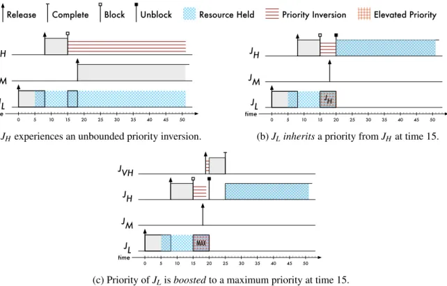
2.1.6.1 Priority Inversions and Progress Mechanisms . . . 28
2.1.6.2 Nested Locking . . . 33
2.1.6.3 Priority-Inversion Blocking . . . 35
2.1.7 Multiprocessork-Exclusion Locking Protocols . . . 37
2.1.7.1 Thek-FMLP . . . 38
2.1.7.2 TheR2DGLP. . . 41
2.1.7.3 TheCK-OMLP. . . 44
2.1.8 Accounting for Overheads in Schedulability Tests . . . 46
2.1.8.1 Preemption-Centric Accounting . . . 47
2.1.8.2 Locking Protocol Overheads . . . 50
2.1.9 Integration of PI-Blocking and Overhead Accounting . . . 52
2.2 Real-Time Operating Systems . . . 54
2.2.1 Basic RTOS Requirements . . . 54
2.2.2 LITMUSRT . . . 56
2.2.3 Interrupt Handling . . . 57
2.2.3.1 Linux . . . 58
2.2.3.2 PREEMPT_RT . . . 60
2.2.3.3 Towards Ideal Real-Time Bottom-Half Scheduling . . . 62
2.3 Review of Embedded GPUs and Accelerators . . . 66
2.4 GPGPU Mechanics . . . 70
2.4.1 Software Architecture . . . 70
2.4.2 Hardware Architecture . . . 74
2.4.2.1 Execution Engine . . . 76
2.4.3 Other Data Transfer Mechanisms . . . 81
2.4.4 Maintaining Engine Independence . . . 83
2.4.5 VectorAddRevisited . . . 85
2.5 Prior Work on Accelerator Scheduling . . . 87
2.5.1 Real-Time GPU Scheduling . . . 87
2.5.1.1 Persistent Kernels . . . 88
2.5.1.2 GPU Kernel WCET Estimation and Control . . . 88
2.5.1.3 GPU Resource Scheduling . . . 90
2.5.2 Real-Time DSPs and FPGA Scheduling . . . 92
2.5.3 Non-Real-Time GPU Scheduling . . . 94
2.5.3.1 GPU Virtualization . . . 94
2.5.3.2 GPU Resource Maximization . . . 96
2.5.3.3 Fair GPU Scheduling . . . 97
2.6 Conclusion . . . 99
Chapter 3: GPUSync . . . 100
3.1 Software Architectures For GPU Schedulers . . . 101
3.1.1 API-Driven vs. Command-Driven GPU Schedulers . . . 101
3.1.2 Design-Space of API-Driven GPU Schedulers. . . 102
3.1.2.1 GPU Scheduling in User-Space . . . 103
3.1.2.2 GPU Scheduling in Kernel-Space . . . 108
3.2 Design . . . 114
3.2.1 Synchronization-Based Philosophy . . . 114
3.2.2 System Model . . . 115
3.2.3 Resource Allocation . . . 115
3.2.3.1 High-Level Description . . . 115
3.2.3.2 GPU Allocator . . . 117
3.2.3.4 Engine Locks . . . 124
3.2.4 Budget Enforcement . . . 127
3.2.5 Integration . . . 130
3.2.5.1 GPU Interrupt Handling . . . 130
3.2.5.2 CUDA Runtime Callback Threads . . . 135
3.3 Implementation . . . 136
3.3.1 General Information . . . 136
3.3.2 Scheduling Policies . . . 137
3.3.3 Priority Propagation . . . 138
3.3.4 Heuristic Plugins for the GPU Allocator . . . 143
3.3.5 User Interface . . . 144
3.4 Conclusion . . . 145
Chapter 4: Evaluation . . . 146
4.1 Evaluation Platform . . . 147
4.2 Platform Configurations . . . 148
4.3 Schedulability Analysis . . . 149
4.3.1 Overhead Measurement . . . 149
4.3.1.1 Algorithmic Overheads . . . 150
4.3.1.2 Memory Overheads . . . 154
4.3.2 Scope . . . 167
4.3.3 Task Model for GPU-using Sporadic Tasks . . . 169
4.3.4 Blocking Analysis . . . 170
4.3.4.1 Three-Phase Blocking Analysis . . . 172
4.3.4.2 Coarse-Grain Blocking Analysis for Engine Locks . . . 172
4.3.4.3 Detailed Blocking Analysis for Engine Locks . . . 174
4.3.4.4 Detailed Blocking Analysis for the GPU Allocator . . . 193
4.3.5.1 Accounting for Interrupt Top-Halves . . . 197
4.3.5.2 Accounting for Interrupt Bottom-Halves . . . 198
4.3.5.3 Limitations . . . 203
4.3.6 Schedulability Experiments . . . 205
4.3.6.1 Experimental Setup . . . 206
4.3.6.2 Results . . . 208
4.4 Runtime Evaluation . . . 221
4.4.1 Budgeting, Cost Prediction, and Affinity . . . 222
4.4.1.1 Budget Performance . . . 223
4.4.1.2 Cost Predictor Accuracy . . . 225
4.4.1.3 Migration Frequency . . . 227
4.4.2 Feature-Tracking Use-Case . . . 228
4.5 Conclusion . . . 234
Chapter 5: Graph Scheduling with GPUs . . . 236
5.1 Motivation for Graph-Based Task Models . . . 237
5.2 PGMRT. . . 240
5.2.1 Graphs, Nodes, and Edges . . . 240
5.2.2 Precedence Constraints and Token Transmission . . . 240
5.2.3 Real-Time Concerns . . . 243
5.3 OpenVX . . . 244
5.4 Adding Real-Time Support to VisionWorks . . . 246
5.4.1 VisionWorks and the Sporadic Task Model . . . 247
5.4.2 Libgpui: An Interposed GPGPU Library for CUDA . . . 252
5.4.3 VisionWorks, libgpui, and GPUSync . . . 252
5.5 Evaluation of VisionWorks Under GPUSync . . . 254
5.5.1 Video Stabilization . . . 254
5.5.3 Results . . . 258
5.5.3.1 Completion Delays . . . 258
5.5.3.2 End-to-End Latency . . . 275
5.6 Conclusion . . . 280
Chapter 6: Conclusion . . . 282
6.1 Summary of Results . . . 282
6.2 Future Work . . . 288
6.3 Closing Remarks . . . 291
LIST OF TABLES
1.1 ADAS prototypes and related research that employ GPUs . . . 7
1.2 Results of experiment reflecting unpredictable and unfair sharing of GPU resources . . . 10
2.1 Summary of sporadic task set parameters . . . 17
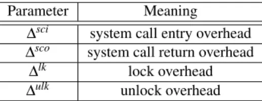
2.2 Summary parameters for describing shared resources . . . 28
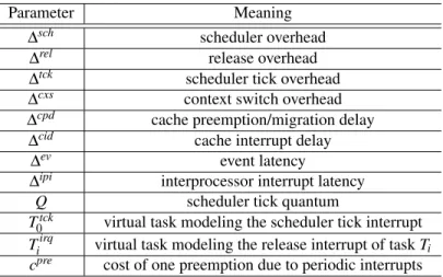
2.3 Summary of parameters used in preemption-centric overhead accounting . . . 49
2.4 Summary of locking protocol overheads considered by preemption-centric accounting . . . 51
2.5 Performance and GPGPU support of several embedded GPUs . . . 67
2.6 NVIDIA software and hardware terminology with OpenCL and AMD equivalents . . . 76
3.1 GPU Allocator heuristic plugin API . . . 144
4.1 Summary of additional parameters to describe and analyze sporadic task sets with GPUs. . . 171
4.2 All possible representative blocking chains that may delay a copy engine request . . . 179
4.3 An example arrangement of copy engine requests . . . 182
4.4 Summary of ILP parameters used for bounding the blocking of copy engine requests . . . 188
4.5 GPUSync configuration rankings under worst-case loaded overheads . . . 210
4.6 GPUSync configuration rankings under worst-case idle overheads . . . 211
4.7 GPUSync configuration rankings under average-case loaded overheads . . . 212
4.8 GPUSync configuration rankings under average-case idle overheads . . . 213
4.9 Migration frequency underC-EDFandC-RMGPUSync configurations . . . 228
5.1 Description of nodes used in the video stabilization graph of Figure 5.8 . . . 256
5.2 Evaluation task set using VisionWorks’ video stabilization demo . . . 257
5.3 Completion delay data forSCHED_OTHER . . . 262
5.4 Completion delay data forSCHED_FIFO . . . 263
5.5 Completion delay data for LITMUSRTwithout GPUSync . . . 263
5.7 Completion delay data for GPUSync for(1,6,PRIO) . . . 264
5.8 Completion delay data for GPUSync for(2,3,FIFO). . . 265
5.9 Completion delay data for GPUSync for(2,3,PRIO) . . . 265
5.10 Completion delay data for GPUSync for(3,2,FIFO). . . 266
5.11 Completion delay data for GPUSync for(3,2,PRIO) . . . 266
5.12 Completion delay data for GPUSync for(6,1,FIFO). . . 267
5.13 Completion delay data for GPUSync for(6,1,PRIO) . . . 267
LIST OF FIGURES
1.1 Historical trends in CPU and GPU processor performance . . . 5
1.2 Host and device code for adding two vectors in CUDA . . . 8
1.3 A schedule ofvector_add() . . . 9
1.4 Matrix of high-level CPU and GPU organizational choices . . . 11
2.1 Example of a PGM-specified graph . . . 18
2.2 PGM-specified graph of Figure 2.1 transformed into rate-based and sporadic tasks . . . 20
2.3 Task ready queues under partitioned, clustered, and global processor scheduling . . . 21
2.4 Example of bounded deadline tardiness for a task set scheduled on two CPUs byG-EDF. . . 25
2.5 Schedule depicting a critical section . . . 27
2.6 Schedules where priority inheritance and priority boosting shorten priority inversions . . . 29
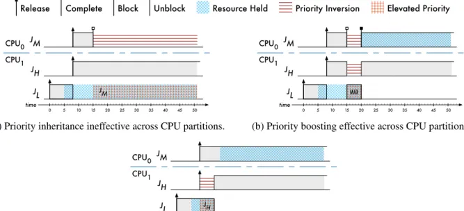
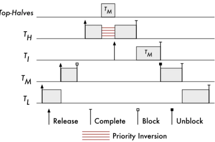
2.7 Situations where multiprocessor systems require stronger progress mechanisms . . . 31
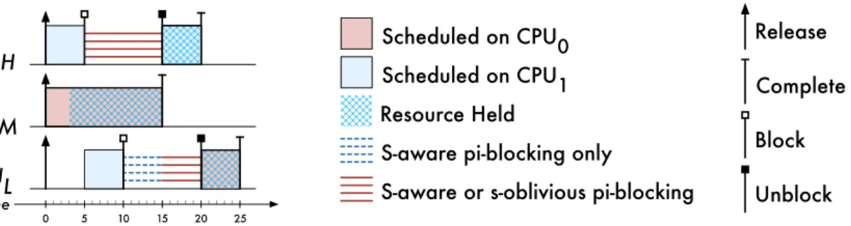
2.8 Comparison of s-oblivious and s-aware pi-blocking under global scheduling . . . 37
2.9 Queue structure of thek-FMLP. . . 39
2.10 Queue structure of theR2DGLP. . . 41
2.11 Queue structure of theCK-OMLP. . . 45
2.12 Schedule depicting system overheads . . . 47
2.13 Fixed-priority assignment when an I/O device is used by a single thread . . . 60
2.14 Example of an unbounded priority inversion . . . 61
2.15 Example of a bounded priority inversion during interrupt bottom-half processing . . . 62
2.16 A pathological scenario for fixed-priority interrupt handling . . . 63
2.17 A priority inversion due to the co-scheduling of a bottom-half . . . 65
2.18 Layered GPGPU software architecture on Linux with closed-source drivers . . . 70
2.19 Situation where a callback thread may lead to a priority inversion . . . 73
2.20 High-level architecture of a modern multicore platform . . . 75
2.21 Code fragments for a three-dimensional CUDA kernel . . . 77
2.23 Decomposition of block threads into warps that are mapped to hardware lanes . . . 79
2.24 Two streams of sequentially ordered GPU operations . . . 83
2.25 Schedule of falsely dependent streamed GPU operations and corrected counterpart . . . 84
2.26 A detailed schedule of host and GPU processing for the simplevector_add()kernel . . . 86
3.1 Software architectures of API-driven GPU schedulers implemented in user-space . . . 104
3.2 Software architectures of API-driven GPU schedulers implemented in kernel-space . . . 110
3.3 High-level design of GPUSync’s resource allocation mechanisms . . . 116
3.4 A schedule of a job using GPU resources controlled by GPUSync . . . 117
3.5 The structure of a GPU allocator lock . . . 118
3.6 Example of budget signal handling . . . 129
3.7 Architecture of GPU tasklet scheduling infrastructure using klmirqd . . . 132
3.8 Memory layout ofnv_linux_state_t . . . 134
3.9 Relative static priorities among scheduling policies . . . 138
3.10 Example of a complex chain of execution dependencies for tasks using GPUSync . . . 139
3.11 Recursive algorithm to propagate changes in effective priority . . . 141
4.1 Concrete examples of multicore, multi-GPU, organizational configurations . . . 148
4.2 PDF of GPU top-half execution time . . . 151
4.3 PDF of GPU bottom-half execution time . . . 152
4.4 CCDFs of top-half and bottom-half execution times . . . 153
4.5 Considered CPMD maximum overheads due to GPU traffic . . . 155
4.6 Considered CPMD mean overheads due to GPU traffic . . . 156
4.7 Increase in considered CPMD overheads due to GPU traffic . . . 159
4.8 GPU data transmission time in an idle system . . . 161
4.9 GPU data transmission time in system under load . . . 162
4.10 Increase in DMA operation costs due to load . . . 164
4.11 Increase in DMA operation costs due to page interleaving . . . 166
4.13 Schedules with overheads due to bottom-half interrupt processing . . . 199
4.14 Schedule depicting callback overheads . . . 201
4.15 Illustrative ranking of configurationA against configurationB. . . 208
4.16 Detailed schedulability result . . . 217
4.17 Detailed result of schedulability and effective utilization . . . 220
4.18 Accumulated execution engine time allocated to tasks . . . 224
4.19 CDFs of percentage error in cost predictions . . . 226
4.20 CDF of job response time forC-EDFwith FIFO-ordered engine locks . . . 231
4.21 CDF of job response time forC-EDFwith priority-ordered engine locks . . . 231
4.22 CDF of job response time forC-RMwith priority-ordered engine locks . . . 232
5.1 Dataflow graph of a simple pedestrian detector application . . . 237
5.2 Transformation of a PGM-specified pedestrian detection application to sporadic tasks . . . 238
5.3 Parallel execution of graph nodes . . . 239
5.4 Construction of a graph in OpenVX for pedestrian detection . . . 245
5.5 Procedure for PGMRT-coordinated job execution . . . 249
5.6 Derivation of PGM graphs used to support the pipelined thread-per-node execution model . . . 250
5.7 Overly long token critical sections may result by releasing tokens at job completion time . . . . 253
5.8 Dependency graph of a video stabilization application . . . 255
5.9 Scenarios that lead to extreme values for measured completion delays . . . 258
5.10 PDF of normalized completion delay data forSCHED_OTHER. . . 271
5.11 PDF of normalized completion delay data forSCHED_FIFO. . . 271
5.12 PDF of normalized completion delay data for LITMUSRTwithout GPUSync . . . 271
5.13 PDF of normalized completion delay data for GPUSync with(1,6,FIFO). . . 272
5.14 PDF of normalized completion delay data for GPUSync with(1,6,PRIO). . . 272
5.15 PDF of normalized completion delay data for GPUSync with(2,3,FIFO). . . 272
5.16 PDF of normalized completion delay data for GPUSync with(2,3,PRIO). . . 272
5.18 PDF of normalized completion delay data for GPUSync with(3,2,PRIO). . . 273
5.19 PDF of normalized completion delay data for GPUSync with(6,1,FIFO). . . 273
5.20 PDF of normalized completion delay data for GPUSync with(6,1,PRIO). . . 273
5.21 CDF of normalized observed end-to-end latency . . . 275
LIST OF ABBREVIATIONS
ADAS Advanced Driver Assistance Systems API Application Programming Interface ASIC Application-Specific Integrated Circuit
BWI Bandwidth Inheritance
CDF Cumulative Distribution Function
CCDF Complementary Cumulative Distribution Function C-EDF Clustered Earliest Deadline First
CE Copy Engine
CK-OMLP Clusteredk-exclusion Optimal Multiprocessor Locking Protocol C++ AMP C++ Accelerated Massive Parallelism
CPU Central Processing Unit
CUDA Compute Unified Device Architecture CVA Compliant Vector Analysis
DAG Directed Acyclic Graph
DGL Dynamic Group Lock
dGPU Discrete Graphics Processing Unit
DMA Direct Memory Access
DPCP Distributed Priority Ceiling Protocol DSP Digital Signal Processor
EDF Earliest Deadline First
EE Execution Engine
FL Fair-Lateness
FMLP Flexible Multiprocessor Locking Protocol FPGA Field Programmable Gate Array
FPS Frames Per Second
G-EDF Global Earliest Deadline First GPC Graphics Processing Cluster
GPGPU General-Purpose Computing on Graphics Processing Units GPU Graphics Processing Unit
HSA Heterogeneous System Architecture iGPU Integrated Graphics Processing Unit IORW Input Output and Read Write IPC Inter-Process Communication IPI Inter-Processor Interrupt ISR Interrupt Service Routine JLFP Job-Level Fixed Priority
k-FMLP k-exclusion Flexible Multiprocessor Locking Protocol MPCP Multiprocessor Priority Ceiling Protocol
MSRP Multiprocessor Stack Resource Policy
NUMA Non-Uniform Memory Access
O-KGLP Optimalk-exclusion Global Locking Protocol OMLP O(m)Multiprocessor Locking Protocol OpenACC Open Accelerators
OpenCL Open Computing Language
OS Operating System
PCIe Peripheral Component Interconnect Express PCP Priority Ceiling Protocol
PDF Probability Density Function P-EDF Partitioned Earliest Deadline First
PGM Processing Graph Method
P2P Peer-to-Peer
RM Rate-Monotonic
RPC Remote Procedure Call
RTOS Real-Time Operating System
R2DGLP Replica-Request Donation Global Locking Protocol
SRP Stack Resource Policy
CHAPTER 1: INTRODUCTION
Real-time systems are those that must satisfy precise timing constraints in order to meet application requirements. We often find such systems where computers sense and react to the physical world. Here, loss of life or property may result if a computer fails to act in the right moment. Real-time system designers must employ algorithms that realize predictable behavior that can be modeled by mathematical analysis. This analysis allows the designer to prove that an application’s timing constraints are met. However, an algorithm can only be as predictable as allowed by the underlying software and hardware upon which it is implemented. Ensuring predictability becomes an increasing challenge as computing hardware grows in complexity. This is especially true for commodity computing platforms, which are optimized for throughput performance—often at the expense of predictability. This challenge is exemplified by the recent development of programmable graphics processing units (GPUs) that are used to perform general purpose computations. GPUs offer extraordinary performance and relative energy efficiency in comparison to traditional processors. However, today’s standard GPU technology is unable to meet basic real-time predictability requirements.
The goal of the research presented in this dissertation is to discover and address the issues that prevent GPUs from being used in real-time systems. GPUs exhibit unique characteristics that are not dealt with easily using methods developed in prior real-time literature. New techniques are necessary. This dissertation presents such techniques that remove the fundamental obstacles that bar the use of GPUs in real-time systems. This research is important because it may allow GPUs to become an enabling technology for embedded real-time systems that tackle computing problems that have been outside the reach of traditional processors.
1.1 Real-Time Systems
The term “real time” has different meaning in different fields. In the context of computer graphics, “real time” often equates to “real fast” or some degree of quality-of-service.1 For instance, a computer graphics animation may be rendered in “real time” if image frames are generated at roughly 30 frames per second. An interactive simulation may be considered “real time” if the simulation runs at about 10 to 15 frames per second. In contrast to these throughput-oriented quality-of-service-based definitions, “real time” in the field of real-time systems is more precise. A real-time system is said to be “correct” if computations meet both logical and temporal criteria. Logical criteria require that the results of a computation must be valid. This condition is true for practically any computational system. Temporal criteria require that these results must also be made available by a designated physical time (hence, “real time”). This strict concern for temporal correctness may not necessarily be included in the aforementioned computer graphics systems where “real fast” is often good enough. Indeed, temporal correctness is as important as logical correctness in a real-time system.
A real-time workload is often embodied by a set of computationaltasks. Each task releases recurring work, with each such release called ajob, according to a predicable rate or time interval. The completion time of each job must satisfy some temporal constraint, such as adeadlinethat occurs within some interval of time after the job’s release. A real-time scheduler is responsible for allocating processor time to each incomplete job. A set of tasks, ortask set, is said to beschedulablewhen timing constraints are guaranteed to always be satisfied.
A scheduling algorithm, in and of itself, does not prove schedulability. Instead, schedulability is formally proven according to an analyticalmodelof the scheduling algorithm and the task set in question. These models may incorporate real-world overheads that are often a function of the scheduling algorithm, the algorithm’s implementation, and the hardware platform upon which jobs are scheduled. Overheads can have a strong effect on schedulability. As a consequence, the design of an efficient real-time system involves the co-designof the analytical model, the scheduling algorithm, and the algorithm’s implementation.
or global. Under partitioned scheduling, each task (and all its associated jobs) is assigned to a processor. Under global scheduling, jobs are free to migrate among all processors. Cluster scheduling is a hybrid of partitioned and global approaches: the jobs of tasks are free to migrate among an assigned subset (or cluster) of processors. Each method may be best suited to a particular application with its own temporal constraints, as there are tradeoffs among the analytical models and associated overheads for each approach.
It is reasonable to assume that many future real-time systems will use multicore processors. Support for real-time GPU computing with multicore processors is a central theme of this dissertation. Moreover, we pay special attention to the interrelations between our analytical models, scheduling algorithms, algorithm implementation, and the computing hardware.
We wish for the results of this dissertation to have bearing on practical applications, so much of the effort behind this dissertation has been on the implementation of real-time multi-GPU schedulers and their integration with real-time multiprocessor (i.e., CPU) schedulers. Implementation and integration is done at the operating system (OS) level. We implement all of our solutions by extending LITMUSRT, a real-time patch to the Linux kernel (Calandrinoet al., 2006; Brandenburg, 2011b, 2014b). This is advantageous since we can use all Linux-based GPGPU software in our research, while also benefiting from LITMUSRT’s variety of real-time multiprocessor schedulers and its other supporting functions.
1.2 Graphics Processing Units
The growth of GPU technology is characterized by an evolutionary process. Early GPUs of the 1970s and 1980s were used to offload 2D rendering computations from the CPU, and support for 3D rendering was common by the end of the 1990s (Buck, 2010). With few exceptions, these GPUs were “fixed function,” meaning that rendering operations were defineda prioriby the GPU hardware. This changed with the advent of the “programmable pipeline” in 2001. The programmable pipeline enables programmers to implement custom rendering operations called “shaders” by using program code that is executed on the GPU. Some of the early successful shader languages include the OpenGL Shading Language (GLSL) (Khronos Group, 2014b), NVIDIA’s “C for Graphics” (Cg) (NVIDIA, 2012), and Microsoft’s High-Level Shader Language (HLSL) (Microsoft, 2014).
GPUs for general-purpose computations was coinedGPGPUby M. Harris in 2002 (Luebkeet al., 2004; Harris, 2009). In early GPGPU approaches, computations were expressed as shader programs, operating on graphics-oriented data (e.g., pixels and vertices). Recognizing the potential of GPGPU, generalized languages and runtime environments were developed by major graphics hardware vendors and software producers to allow general purpose programs to be run on graphics hardware without the limitations imposed by graphics-focused shader languages. Notable platforms include the Compute Unified Device Architecture (CUDA) (NVIDIA, 2014c), OpenCL (Khronos Group, 2014a), and OpenACC (OpenACC, 2013). The ease of use enabled by these advances has facilitated the adoption of GPGPU in a number of fields of computing. Today, GPGPU is used to efficiently handle data-parallel compute-intensive problems such as cryptography (Harrison and Waldron, 2008), supercomputing (Meueret al., 2014), finance (Scicomp Incorporated, 2013), ray-tracing (Aila and Laine, 2009), medical imaging (Watanabe and Itagaki, 2009), video processing (Pieterset al., 2009), and many others.
GPGPU technology has received little attention in the field of real-time systems, despite strong motiva-tions for doing so. The strongest motivation is that the use of GPUs can significantly increase computational performance. This is illustrated in Figure 1.1(a), which depicts performance trends of high-end Intel CPUs and NVIDIA GPUs over much of the past decade (NVIDIA, 2014c; Intel, 2014; Onget al., 2010). Figure 1.1(a) plots the peak theoretical single-precision performance in terms of billions of floating point operations per second (GFLOPS). There is a clear disparity between CPU and GPU performance in favor of GPUs. For example, NVIDIA’s Titan GTX Black GPU can perform at 5,121 GFLOPS in comparison to 672 GFLOPS for the Intel Ivy Bridge-EX—the GPU has a 7.6 times greater throughput.
This disparity is even greater when we consider mobile CPUs, such as those designed by ARM. For instance, the ARM Cortex-A15 series processor as a peak theoretical performance of 8 GFLOPs at 1GHz (Ra-jovicet al., 2014). Thus, the dual Cortex-A15 cores of Samsung’s Exynos 5250 (which runs as 1.7GHz) collectively achieve 27.2 GFLOPS. In contrast, the embedded NVIDIA K1 and PowerVR GX6650 GPUs can both achieve a reported 384 GFLOPS (Smith, 2014a), making them more than 14 times faster than the Exynos 5250.2
Growth in raw floating-point performance does not necessarily translate to equal gains in performance for actual applications. In the case of both CPUs and GPUs, observed theoretical performance only nears 2It is unfair to compare the Titan GTX Black to any embedded processor since the GPU requires a great deal more power. The Titan
0 1000 2000 3000 4000 5000 6000
Jan-03 Jan-04 Jan-05 Jan-06 Jan-07 Jan-08 Jan-09 Jan-10 Jan-11 Jan-12 Jan-13 Jan-14
T he ore ti ca l P ea k G F L O P S Date Trends in GFLOPS
CPU (Intel) GPU (NVIDIA)
6800 Ultra 7800 GTX 8800 GTX GTX-260 GTX-280 GTX-480 GTX-580 GTX-680 TITAN GTX
TITAN GTX Black
Harpertown Bloomfield Westmere-EX Sandy Bridge-EP
Ivy Bridge-EX
(a) Trend in GFLOPS.
0 5 10 15 20 25
Jan-03 Jan-04 Jan-05 Jan-06 Jan-07 Jan-08 Jan-09 Jan-10 Jan-11 Jan-12 Jan-13 Jan-14
W at ts pe r T he ore ti ca l P ea k G F L O P S Date
Trends in GFLOPS-per-Watt
CPU (Intel) GPU (NVIDIA)
ClovertownHarpertown Bloomfield
Westmere-EX Sandy Bridge-EP
Irwindale
Ivy Bridge-EX 8800 GTX
GTX-260GTX-280 GTX-480 GTX-580
GTX-680 TITAN GTX
TITAN GTX Black
(b) Trend in GFLOPS-per-Watt.
Figure 1.1: Historical trends in CPU and GPU processor performance.
real-time systems, computations accelerated by GPUs may execute at higher frequencies or perform more computation per unit time, possibly improving system responsiveness or accuracy.
Power efficiency is another motivation to use GPUs in real-time systems, since real-time constraints often must be satisfied in power-constrained embedded applications. GPUs can carry out computations at a fraction of the power needed by CPUs for equivalent computations. This is illustrated in Figure 1.1(b), which depicts the GFLOPS-per-watt for the same performance points of Figure 1.1(a). Here, the Titan GTX Black can perform roughly 20.5 GFLOPS per watt in comparison to 4.3 GFLOPS per watt of the Ivy Bridge-EX—the GPU is 4.7 times more efficient. For an additional point of reference, the K1 and GX6650 integrated GPUs perform approximately 48 GFLOPS-per-watt, while the Exynos 5250 CPUs deliver approximately 6.8 GFLOPS-per-watt.3
1.3 Real-Time GPU Applications
There are several application domains that may benefit from real-time support for GPUs. For example, real-time-scheduled GPUs may be employed to realize predictable video compositing and encoding for use in live news and sports broadcasting (NVIDIA, 2014e). Another domain includes support of high frequency trading and other time-sensitive financial applications (Kinget al., 2010). However, possibly the greatest potential for GPUs in real-time systems is in future automotive applications.
The domain that may benefit the most from real-time support for GPUs is in the advanced driver assistance systems (ADAS) of new and future automobiles. Here, vehicle computer systems realize “intelligent” alert and automated features that improve safety and/or the driving experience. For example, a system that alerts the driver of pedestrians in the path of the vehicle is an ADAS. An intelligent adaptive cruise control system that can automatically steer the vehicle and control its speed in stop-and-go highway traffic is another. Other ADAS features include automatic traffic sign recognition, obstacle avoidance, and driver fatigue detection. There are clear safety implications to ADAS: if the vehicle fails to act in the right moment, loss of life may result. Precise timing constraints must be met.
Common to these ADAS applications is a reliance upon a rich sensor suite. This includes video cameras, radar detectors, acoustic sensors, and lidar4sensors (Weiet al., 2013). Together, these sensors generate an 3Power metrics for individual components of embedded processors are difficult to find. Here, we conservatively assume that the K1, GX6650, and Exynos 5250 each consume eight watts. This a common limit for the entirety of a smartphone- and tablet-class chip, of which GPU and CPUs are merely components.
Application Prototypes and Research
Pedestrian, Vehicle, and Zhang and Nevatia (2008); Wojeket al. (2008) Obstacle Detection Baueret al. (2010); Benensonet al. (2012) Traffic Sign Recognition Mussiet al. (2010); Muyan-Ozceliket al. (2011) Driver Fatigue Detection Lalondeet al. (2007)
Lane Following Hommet al. (2010); Kuhnlet al. (2012) Seo and Rajkumar (2014) Table 1.1: ADAS prototypes and related research that employ GPUs.
enormous amount of data for an embedded vehicle computing system to process. It is too much in fact for traditional computing hardware to handle within a vehicle’s size, weight, and power (SWaP) constraints, much less being affordable. GPUs offer a viable alternative because many of the algorithms employed in ADAS are data parallel—ideal for GPUs. This is especially true of computer vision algorithms that operate upon video camera feeds and the point-cloud processing of LIDAR data.
Researchers have begun applying GPUs to ADAS problems, as illustrated by Table 1.1, which lists several ADAS prototypes and related research that uses GPUs. However, each prototype assumes full control of theentirecomputing system; computing resources such as CPUs and GPUs are not shared with other tasks. This does little to resolve automotive SWaP or cost constraints. If advanced automotive features are to be realistically viable, then such computations must be consolidated onto as few low-cost CPUs and GPUs as possible, while still meeting timing constraints. The design and implementation of foundational real-time methods for such systems is the focus of this dissertation research.
1.4 An Introduction to GPGPU Programming
A brief introduction to GPGPU programming is necessary to conceptualize the challenges of using GPUs in real-time systems. We first present a high-level description of GPGPU programming and GPU mechanics. We then discuss the limitations that prevent us from using GPUs in a real-time system without any specialized real-time mechanisms.
1.4.1 GPGPU Programming
1 // Add v e c t o r s ‘ a ’ and ‘ b ’ of ‘ n u m _ e l e m e n t s ’ f l o a t s and s t o r e r e s u l t s in ‘ c ’
2 // u s i n g a G P U .
3 v o i d v e c t o r _ a d d ( f l o a t * a , f l o a t * b , f l o a t * c , int n u m _ e l e m e n t s ) {
4 f l o a t * gpu_a , * gpu_b , * g p u _ c ;
5
6 . . . // a l l o c a t e GPU - s i d e m e m o r y for ‘ g p u _ a ’ , ‘ g p u _ b ’ , and ‘ g p u _ c ’
7
8 // c o p y c o n t e n t s of ’ a ’ and ’ b ’ to c o r r e s p o n d i n g b u f f e r s on the GPU
9 c u d a M e m c p y ( gpu_a , a , n u m _ e l e m e n t s * s i z e o f ( f l o a t ));
10 c u d a M e m c p y ( gpu_b , b , n u m _ e l e m e n t s * s i z e o f ( f l o a t ));
11
12 // p e r f o r m ‘ g p u _ c [ i ] = g p u _ a [ i ] + g p u _ b [ i ] ’ for i in [0 . . n u m _ e l e m e n t s )
13 g p u _ v e c t o r _ a d d < < <. . .> > >( gpu_a , gpu_b , gpu_c , n u m _ e l e m e n t s );
14
15 // c o p y the r e s u l t s of v e c t o r A d d s t o r e d in ‘ g p u _ c ’ to b u f f e r ‘ c ’
16 c u d a M e m c p y ( c , gpu_c , n u m _ e l e m e n t s * s i z e o f ( f l o a t ));
17
18 . . . // f r e e b u f f e r s a l l o c a t e d to ‘ g p u _ a ’ , ‘ g p u _ b ’ , and ‘ g p u _ c ’
19 }
(a) Host code for adding vectors, using a GPU.
1 // GPU r o u t i n e for a d d i n g e l e m e n t s of v e c t o r s ‘ a ’ and ‘ b ’ w i t h r e s u l t s t o r e d ‘ c ’
2 _ _ g l o b a l _ _
3 v o i d g p u _ v e c t o r _ a d d ( f l o a t * a , f l o a t * b , f l o a t * c , int n u m _ e l e m e n t s ) {
4 int i = b l o c k D i m . x * b l o c k I d x . x + t h r e a d I d x . x ;
5 if ( i < n u m _ e l e m e n t s ) {
6 c [ i ] = a [ i ] + b [ i ];
7 }
8 }
(b) Device kernel for adding vectors.
Figure 1.2: Host and device code for adding two vectors in CUDA.
the case where GPUs are equipped with their own memory, memory copies between CPU main memory and GPU-local memory.
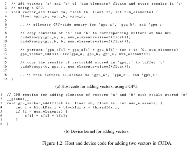
GPU (or “device”) code is invoked by CPU (or “host”) code, in a manner similar to a remote procedure call (RPC). Device-side procedures are commonly referred to as “kernels.”5 A simple GPGPU routine (in the CUDA language) for adding the elements of two arrays (or vectors) is given in Figure 1.2. Host code appears in Figure 1.2(a) and device code in Figure 1.2(b). The routinevector_add()executes on the host. In lines 9 and 10 of Figure 1.2(a), memory is copied from host memory to device memory as input for the gpu_vector_add()kernel. In line 13, this kernel is called by the host, triggering the procedure in Figure 1.2(b) to execute on the device. The kernel’s output resides in device memory after it completes. The resulting output of the kernel is copied back to host memory on line 16 of Figure 1.2(a).
A simplified schedule for the VectorAdd routine is depicted in Figure 1.3. (The actual sequence of operations is more complex, as we shall see in Chapter 2, but this level of detail is sufficient for now.) From 5This unfortunate name should not be confused with an operating system kernel. A GPU kernel and operating system kernel have
CE
EE
CPU
time
t
1 t2 t3 t4 t5 t6 t7 t8 t9
vector_host(…)
cudaMemcpy(gpu_a, a,…);
cudaMemcpy(gpu_b, b,…); cudaMemcpy(c, gpu_c,…); gpu_vector_host(…)
Figure 1.3: A schedule ofvector_add().
this schedule, we see thatvector_add()begins execution on a CPU, starting at timet1. The memory copy operations are carried out using direct memory access (DMA) by a “Copy Engine” (CE) processor on the time intervals[t2,t3],[t4,t5], and[t8,t9]. The CE is a GPU component used for DMA memory operations. The kernelgpu_vector_add()executes on the GPU’s “Execution Engine” (EE) during the time interval [t6,t7]. (We discuss CEs and EEs in more depth in Chapter 2.) Observe that the CPU code waits for each
GPU-related operation to complete—indicated by a set of horizontal dashed lines. During these intervals, the CPU code may suspend or spin while waiting for GPU operations to complete (the particular desired behavior may be specified by the programmer).
1.4.2 Real-Time GPU Scheduling
Thread Loop Counts Run 1 Run 2 Run 3
1 0 0 0
2 104 969 0
3 1,307 0 3,706
4 2,230 1,928 0
5 0 786 0
Total 3,641 3,683 3,706 Table 1.2: Reported loop counts.
Unfortunately, stock GPGPU technology offers little support for dependable scheduling policies. Con-tention for GPU resources is often resolved through undisclosed arbitration policies. These arbitration policies typically have no regard for task priority and may exhibit behaviors detrimental to multitasking on host CPUs. Furthermore, a single task can dominate GPU resources by issuing many or long-running operations. Allocation methods are needed that eliminate or ameliorate these problems. We demonstrate several of these points with a simple experiment.
In this experiment, we have a program that repeatedly executes the VectorAdd routine on 4,000, 000-element vectors in a tight loop. We ran five instances of our program, as threads, concurrently under Linux’s general purpose scheduler (e.g., a non-real-time scheduler). Our test platform has more CPUs than test threads, but all threads share the same GPU (an NVIDIA Quadro K5000). Our threads execute for a duration of 30 seconds and report the number of completed loop iterations upon completion. Table 1.2 gives the reported loop counts for three separate test runs of our experiment. We observe two important behaviors in this data. First, by comparing the values within each column, we see that each thread receives a very uneven share of GPU resources. For instance, in Run 1, Thread 2 completes 104 loops while Thread 4 completes 2,230. Second, by comparing the values within each row, we see that each thread receives a different amount of GPU resources in each experiment. For example, Thread 3 is starved in Run 2, but it receivesallof the GPU resources in Run 3. In short, GPU resources are allocatedunfairlyandunpredictably.
CPU Scheduling G PU O rg a n iz a tio n
Partitioned Clustered Global
P a rt it io n e d C lu st e re d G lo b a l
Figure 1.4: Matrix of high-level CPU and GPU organizational choices.
devise and implement mechanisms that satisfy our need for predictability while still using the manufacturer’s original software.
1.4.3 Real-Time Multi-GPU Scheduling
Modern hardware can support computing platforms that have multiple GPUs. Given the performance benefits GPUs offer, it is desirable to support multi-GPU computing in a real-time system. Similar to CPUs in multiprocessor scheduling, GPUs can be organized following a partitioned, clustered, or global approach. When combined with the earlier-discussed multiprocessor scheduling methods, we have nine high-level possible allocation categories, as illustrated in matrix form in Figure 1.4. Can real-time mechanisms be devised to support every configuration choice? Which configurations are best for real-time predictability? Which configurations offer the best observed real-time performance at runtime? Do configuration choices really matter? The answers to these basic questions are not immediately clear. This dissertation investigates these questions in depth.
1.5 Thesis Statement
This dissertation seeks to investigate real-time GPU scheduling and demonstrate the benefits of GPGPU in real-time systems. To this end, we put forth the following thesis statement:
The computational capacity of a real-time system can be greatly increased for data-parallel
applications by the addition of GPUs as co-processors, integrated using real-time scheduling and
synchronization techniques tailored to take advantage of specific GPU capabilities. Increases in
computational capacity outweigh costs, both analytical and actual, introduced by management
overheads and limitations of GPU hardware and software.
1.6 Contributions
We now present an overview of the contributions of this dissertation that support this thesis.
1.6.1 A Flexible Real-Time Multi-GPU Scheduling Framework
The central contribution of this dissertation is the design of a flexible real-time multi-GPU scheduling framework. In Chapter 3, we present our framework, which is called GPUSync. We posit that GPU management is best viewed as a synchronization problem rather than one of scheduling. At its heart, GPUSync is a novel combination and adaptation of several recent advances in multiprocessor real-time synchronization made by Brandenburget al. (2011) and Wardet al. (2012, 2013). This approach provides us established techniques for enforcing real-time predictable and an analytical framework for testing real-time schedulability.
GPUSync is highly configurable and supports every high-level CPU/GPU scheduling/organizational method depicted in Figure 1.4. For each high-level configuration, a system designer may select a low-level GPUSync configuration that best complements their analytical model or yields the best observed runtime performance (or perhaps both).
1.6.2 Techniques for Supporting Closed-Source GPGPU Software
In Chapter 2, we identify issues that may arise when we attempt to use non-real-time GPGPU software in a real-time system. Specifically, these issues relate to:(i)non-real-time resource arbitration, and(ii)the real-time scheduling of GPU device driver and GPGPU runtime computations.
We present a solution to these problems in Chapter 3. We resolve the arbitration issues of(i)bywrapping the GPGPU runtime with our own interface to GPUSync. Resource contention is already resolved when the GPGPU runtime is invoked by application code. Thus, our real-time system is no longer at the mercy of undisclosed non-real-time arbitration techniques. We address the scheduling problems of(ii)through interceptiontechniques. For example, we intercept the OS-level interrupt processing of the GPU device driver and insert our own interrupt scheduling framework. We also intercept the creation of “helper” threads created by GPGPU runtime and assign them proper real-time scheduling priorities. These features integrate with GPUSync, allowing the framework to dynamically adjust scheduling priorities in order to maintain real-time predictability.
1.6.3 Support for Graph-Based GPGPU Applications
In Chapter 5, we extend real-time GPGPU support to graph-based software architectures, strengthening the relevance of GPUs in real-time systems. In such architectures, vertices represent sequential code segments that operate upon data, and edges express the flow of data among vertices. The flexibility offered by such an architecture’s inherent modularity promotes code reuse and parallel development. Also, these architectures naturally support concurrency, since parallelism can be explicitly described by the graph structure. This allows work to be scheduled in parallel and take advantage of the pipelined execution of graph processing— techniques known to improve analytical schedulability and runtime behavior.
1.6.4 Implementation and Evaluation
In Chapter 3, we also describe the implementation of GPUSync in LITMUSRT. We discuss several of the unique implementation-related challenges we addressed, including efficient locking protocols, budget enforcement techniques, and the tracking of real-time priorities.
In Chapters 4 and 5, we evaluate our implementation in terms of analytical schedulability and runtime performance. The results of this evaluation support the central claim of this dissertation’s thesis that GPUs can be used in a real-time system, resulting in increased computational capacity.
In order to evaluate schedulability, we develop and present an analytical model of real-world system behavior under GPUSync in Chapter 4. This model incorporates carefully measured empirical overheads relating to real-time scheduling and GPU operations. Using this model, we carry out schedulability experi-ments in order to determine the most promising configurations of GPUSync. This evaluation is broad and is backed by data generated from tens of thousands of CPU hours of experimentation. Ultimately, we find that clustered CPU scheduling with partitioned GPUs offers the best real-time schedulability, overall. However, clustered GPU scheduling is competitive in some situations.
We demonstrate the effectiveness of our real-time GPU scheduling techniques by observing the run-time behavior of GPUSync under several synthetic and “real-world application” scenarios in Chapters 4 and 5. Among our findings, we show that although partitioned GPU scheduling may offer better real-time schedulability, clustered GPU scheduling may offer better observed real-time behavior.
1.7 Organization
CHAPTER 2: BACKGROUND AND PRIOR WORK1
In this chapter, we discuss background material and prior work on topics related to this dissertation. We begin with a discussion of real-time multiprocessor scheduling, locking protocols, and schedulability analysis. We then examine prior work on the implementation of real-time schedulers in real-time operating systems (RTOSs) and issues related to peripheral device management (specifically, device interrupt handling). We then review the current state of accelerator co-processors in the embedded domain to help motivate the timeliness of our research. We then delve into relevant aspects of GPU hardware and software architectures and programming models. Here, we also discuss the challenges of real-time GPU computing. We conclude with a review of related prior work on GPU scheduling.
2.1 Multiprocessor Real-Time Scheduling
We discuss several foundational elements of real-time multiprocessor scheduling in this section. We begin with a description of the analytical approach we use to model real-time workloads in this dissertation. This is followed by a discussion of the meaning of the term “schedulability” and the procedures we use for formally proving real-time correctness. We then examine the topic of resource sharing in real-time systems, and how sharing may impact schedulability analysis. Finally, we discuss the methods we use to account for real-world system overheads in schedulability analysis.
2.1.1 Sporadic Task Model
A workload that is run on a real-time system is said to be schedulable when guarantees on timing constraints can be made. Schedulability is formally proved through analytical models. One such model is the well-studiedsporadic task model(Mok, 1983); we focus on this task model in this research. We define the 1Portions of this chapter previously appeared in the proceedings of two conferences. The original citations are as follows:
Elliott, G. and Anderson, J. (2012a). The limitations of fixed-priority interrupt handling in PREEMPT_RT and alternative approaches. InProceedings of the 14th OSADL Real-Time Linux Workshop, pages 149–155;
basic elements of the sporadic task model here. Later in this section, we expand this model to incorporate resource sharing. In Chapter 4, we further expand the model to describe GPUs and GPGPU workloads.
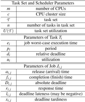
Under the sporadic task model, we describe the computational workload as atask set,T, that is specified as a collection ofn tasks: T ,{T1,· · ·,Tn}. Ajobis a recurrent invocation of work by a task, Ti, and is denoted byJi,j, where jindicates the jthjob ofTi(we may omit the subscript jif the particular job invocation is inconsequential). TaskTiis described by a tuple of three parameters:(ei,pi,di). The worst-case execution time (WCET) of a job is given byei. The releases of jobsJi,jandJi,j+1have a minimum release separation time described by the task’speriod, pi. A task is said to beperiodic(instead of sporadic) if its jobs are always separated bypitime units. JobJi,jis released (arrives) at timeai,j and completes (finishes) at time fi,j. Each job has aprecedence constraint: although jobJi,j+1may be released before jobJi,j completes,Ji,j+1 cannot be scheduled until after fi,j. Apendingjob is an incomplete released job that has had its precedence constraint met. Theresponse timeofJi,jis
ri,j, fi,j−ai,j. (2.1)
Every task has arelative deadline,di. A task is said to have an implicit, constrained, or arbitrary deadline if di=pi,di≤pi, ordi≥0, respectively. Every job has anabsolute deadline, defined by
Di,j,ai,j+di. (2.2)
Each job must execute for at mosteitime units in order to complete, and it must receive this execution time byDi,jto meet its deadline. We definelatenessby
li,j, fi,j−Di,j. (2.3)
Deadlinetardinessis defined by
xi,j,max(0,li,j). (2.4)
Theutilizationof a task quantifies the long-term processor share required by the task and is given by the term
ui, ei
Task Set and Scheduler Parameters
m number of CPUs
c CPU cluster size
T task set
n number of tasks in task set
U(T) task set utilization
Parameters of TaskTi
ei job worst-case execution time
pi period
di relative deadline
ui utilization
Parameters of JobJi,j
ai,j release (arrival) time
fi,j completion (finish) time
Di,j absolute deadline
ri,j response time
li,j deadline lateness (may be negative)
xi,j deadline tardiness
Table 2.1: Summary of sporadic task set parameters.
The total utilization of a task set is given by
U(T) = n
∑
i=1
ui. (2.6)
Table 2.1 summarizes the various parameters we use in modeling a sporadic task set.
2.1.2 Rate-Based Task Model
Therate-based task modelprovides a similar approach to describing the workload of a real-time system as the sporadic task model (Jeffay and Goddard, 1999). Instead of usingpito describe the arrival sequence of taskTi’s jobs, we useχito specify the maximumnumberof jobs of taskTi that may arrive within a time window ofυitime units.2 Thus, each task is described by a tuple of four parameters:(ei,χi,υi,di). We reuse all of the sporadic task model parameters we described earlier, except forpiandui. Utilization is given by
urbi ,ei·
χi
υi
. (2.7)
2Jeffay and Goddard use the symbolsx
G
2iG
3iG
4iG
1i̺2i←1= 4 ϕ2i←1= 7 κ2i←1= 3
̺3i←1= 4 ϕ3i←1= 5 κ3i←1= 3
̺4i←2= 1 ϕ4i←2= 3 κ4i←2= 2
̺4i←3= 2 ϕ4i←3= 6 κ4i←3= 4
Figure 2.1: Example of a PGM-specified graph (courtesy of Liu and Anderson (2010)).
We do not use the rate-based task model directly to determine schedulability in this dissertation. However, we do use it as anintermediaryrepresentation in the process of transforming a more complicated real-time model into the sporadic task model. We discuss this next.
2.1.3 Processing Graph Method
The sporadic and rate-based task models are limited in that they describe a set of independent tasks. However, real-time workloads are not always so simple. For example, the sporadic and rate-based task models lack the necessary expressiveness to describe the scenario where the input of a job of one taskTiis dependent upon the output of a job of another taskTj. We see this type of inter-task dependence in graph-based software architectures. The Processing Graph Method (PGM) is an expressive model for describing such software architectures.
PGM describes the dependencies among jobs in terms of producer/consumer relationships. The workload is described by set ofn graphs: G,{G1,· · ·,Gn}. Each graph is comprised of subtasks,Gi,{G1i,· · ·,G
zi
edge connectingGij andGki before a job ofGki may execute is given byϕik←j. We denote the set of subtasks
that directly generate input forGij with the functionpred(Gij). Likewise, we denote the set of subtasks that directly consume the output ofGijwith the functioncons(Gij). We attach rate-based arrival parameters to the source nodes of each graph. Similar to the rate-based task model, we useχijto specify the maximumnumber
of jobs of taskGijthat may arrive within a time window ofυijtime units.
Goddard presents a procedure for transforming a set of PGM graphs into a rate-based task set in his Ph.D. dissertation (Goddard, 1998). Building upon this work, Liu and Anderson developed a method to transform the PGM-derived rate-based task set into a sporadic task set, provided that the underlying graph contains no cycles (i.e., a directed acyclic graph (DAG)) (Liu and Anderson, 2010).
We now present the procedure for transforming a PGM-based graph into a sporadic task set, via an intermediate transformation into a rate-based task set. We direct the reader to Goddard (1998) and Liu (2013) for the justifications behind the graph-to-rate-based-task-set and rate-based-to-sporadic-task-set transformations, respectively.
We first assume that rate-based arrival parameters have been assigned to all source nodes of every graph. We then derive these parameters for the remaining nodes using the equations
υik,lcm
κik←v·υiv
gcd(%k←v
i ·χiv,κik←v)
|v∈pred(Gki)
, (2.8)
χik,υ k i ·
%k←v i
κik←v ·χ
v i
υiv, whereG
v
i ∈pred(G k
i). (2.9)
We compute a relative deadline for every task using the equation:
dik,υ k i
χik. (2.10)
At the end of this transformation, we have a rate-based task set,Trb, derived fromG. We transformTrbinto a sporadic task set by replacing the termsχikandυikof each task with a period equal to each task’s relative
deadline:
pki ,υ k i
(e1i,1,4,4)
(a) Rate-based transformation.
Ti2 = (e2i,3,3)
Ti3 = (e3i,3,3)
Ti4 = (e4i,6,6) Tik = (eki, pki, dki)
Ti1 = (e1i,4,4)
(b) Sporadic transformation.
Figure 2.2: PGM-specified graph of Figure 2.1 transformed into rate-based (a) and sporadic (b) tasks.
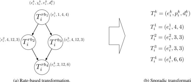
Example 2.1. Consider the PGM-specified graph in Figure 2.1. Let us assume thatG1i has an execution rate of (χi1=1,υi1=4).3 We now transform the graphGi into a set of rate-based tasks, followed by a transformation into sporadic tasks. These transformations are illustrated in Figure 2.2.
We apply Equations (2.8) and (2.9) to find υi2 =lcm
n
3·4 gcd(4·1,3)
o
=12 and χi2 =12·4·13·4 =4 for the rate-based task Trb2
i . We use Equation (2.10) to find that the relative deadline for T rb2
i is di2 = 12
4 =3. The rate-based task T rb3
i is similarly defined, since κ 2←1
i =κi3←1 and %2←1i =%3←1i . Also,
υi4=lcm
n
2·12 gcd(4,2),
4·12 gcd(8,4)
o
=lcm{12,12}=12 andχi4=12·1 2·
4
12=2 for the rate-based taskT rb4
i . The relative deadline isd4i = 12
2 =6. To transform the rate-based tasks to sporadic tasks, we merely take the
rate-based relative deadline as the period for each task. ♦
Although we model the derived sporadic task set as a set of independent tasks, a scheduler must take steps, at runtime, to(i)efficiently track the production and consumption of tokens on each edge; and(ii)dynamically adjust the release time of jobs to ensure token input constraints are satisfied. We may accomplish(i)by enabling token-producing jobs to notify the scheduler of when token constraints are satisfied. Liu and Anderson (2010) specify how to address(ii): we delay the release of any sporadic job until inputs are satisfied. Suppose a jobJik,j is “released” at timeaki,j as a conventional sporadic task, but that the token constraints ofJik,j are not satisfied until a later time,t. In such a case, we adjust the release time of jobJik,j toaki,j=t and its deadline toDki,j=t+dik. We present an efficient implementation for token constraint tracking and release-time adjustment in Chapter 5.
CPU 0 CPU 1 CPU 2 CPU 3
(a) Partitioned (c=1)
CPU 0 CPU 1 CPU 2 CPU 3
(b) Clustered (c=2)
CPU 0 CPU 1 CPU 2 CPU 3
(c) Global (c=4)
Figure 2.3: Each processor cluster is fed by a dedicated ready queue of jobs. Example withm=4.
2.1.4 Scheduling Algorithms
We now discuss the algorithms we use to schedule a given sporadic task set on set of processors, as well as the formal analysis we use to determine whether timing constraints can be met.
The task setT is scheduled on hardware platform consisting ofmprocessors (or cores). These processors may be divided into disjoint clusters ofcprocessors each. Each task (and all its associated jobs) is assigned to a cluster. Whenc=1, 1<c<m, orc=m, the multiprocessor system is said to be scheduled by a partitioned, clustered, or global scheduler, respectively.
An incomplete released job isreadyif it is available for execution, it isscheduledif the job is executing on a processor, and it issuspendedif the job cannot be scheduled (for whatever reason). A scheduled job is eitherpreemptibleornon-preemptible, and cannot be descheduled while it is non-preemptible.
Each processor cluster draws ready jobs from a dedicated priority-ordered ready queue. This is depicted in Figure 2.3 for a system with four processors under partitioned (inset (a)), clustered (inset (b)), and global (inset (c)) scheduling. In this figure, each ready job is depicted by a different shaded box. Jobs enter the ready queue when they are released, resume from a suspension, or are preempted. Jobs exit the ready queue when they are scheduled. A job is free to migrate among all processors within its assigned cluster. Of course, no migration is possible under partitioned scheduling, since each cluster is made up of only one processor.
of every task may have a different priority. The rate-monotonic (RM) scheduler prioritizes tasks with shorter periods over those with longer ones. Similarly, the deadline-monotonic (DM) scheduler prioritizes tasks according to relative deadlines instead of period. Period and relative deadline parameters are constant, so RM and DM are FP schedulers. The earliest-deadline-first (EDF) scheduler prioritizes jobs with earlierabsolute deadlines over those with later ones. EDF is a dynamic-priority scheduler since the absolute deadline depends upon the release time of a job. Similarly, the recently developed “fair-lateness” (FL) scheduler prioritizes jobs using pseudo-deadlines calledpriority points(Erickson, 2014). The relative priority point of a task, denoted by the parameteryi, is determined by the following formula:
yi,di− m−1
m ei. (2.12)
Similarly, an absolute priority point of a job, denoted by the parameterYi,j, is given by:
Yi,j,Di,j− m−1
m ei. (2.13)
FL is also a dynamic-priority scheduler.
We combine the processor cluster organization with a prioritization scheme to create a multiprocessor scheduling algorithm. For example, we refer to the multiprocessor scheduler defined by combination of partitioned processor organization (c=1) with EDF prioritization as “partitioned EDF” (P-EDF). Likewise, we get the “global RM” (G-RM) scheduler by combining globally organized processors (c=m) with RM prioritization.
2.1.5 Schedulability Tests and Tardiness Bounds
A schedule isfeasiblefor a task set if all timing constraints are met. A task set isschedulableunder a given scheduling algorithm if the algorithm always generates a feasible schedule. (A scheduling algorithm is optimal if it always generates a feasible schedule, if one exists.) Our definitions of feasibility and schedulability are with respect to some notion of “timing constraints”—these may be application-specific. We call systems wherealldeadlines must be methard real-time(HRT) systems. Applications with HRT requirements are found in safety-critical applications where loss of life or damage may occur if a deadline is missed. We call systems where some deadline misses are acceptablesoft real-time(SRT) systems. A video decoder is an example of an application with SRT requirements. This definition of SRT remains general and can be further refined. In the context of this dissertation, an SRT system is one where deadline tardiness (the margin by which a deadline may be missed) isbounded.
Aschedulability testis a procedure that determines if a given task set is schedulable. For instance, a classic result from a seminal work by Liu and Layland (1973) states that any periodic task set scheduled by uniprocessor RM scheduling is HRT-schedulable if
U(T)≤n(21n −1). (2.14)
This schedulability test is only sufficient, as some task setsmaybe schedulable with utilizations greater thann(21n−1). In the same work, Liu and Layland also showed that any periodic task set scheduled under
uniprocessor EDF scheduling is HRT-schedulable iff
U(T)≤1. (2.15)
Since any task set with a utilizationgreaterthan one has no feasible schedule, uniprocessor EDF is an optimal scheduler.
sporadic task set is schedulable with bounded deadline tardiness if the constraints
U(T)≤m (2.16)
and
∀Ti: ui≤1 (2.17)
hold true. Inequality (2.16) defines the task set utilization constraint, and Inequality (2.17) defines a per-task utilization constraint. These constraints can also be used to evaluate the schedulability (with bounded tardiness) of task sets with arbitrary deadlines (Erickson, 2014).
We can compute deadline tardiness bounds for schedulable implicit-deadline task sets. We define several terms and functions in order to describe this process. Leteminbe the smallest job execution time among the tasks inT. We useE(T)to define an operation that returns the subset ofm−1 tasks inT with the largestej. Similarly, we useU(T)to define an operation that returns the subset ofm−2 tasks inT with the largestuk. The deadline tardiness of any job is bounded by
xi=ei+(∑Tj∈E(T)ej)−emin
m−∑Tk∈U(T)uk
. (2.18)
We may extend the above test and tardiness bounds toC-EDFby testing each cluster individually.
In cases wheredU(T)e<m, we may obtain tighter tardiness bounds by substituting the termmwithmb,
where
b
m,dU(T)e, (2.19)
in Equation (2.18) and the definitions ofE(T)andU(T). This optimization reflects the observation that a task set only requiresdU(T)eprocessors to be schedulable with bounded tardiness. The bound provided by Equation (2.18) may be tightened if we assumefewerthanmprocessors in analysis.
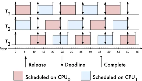
Example 2.2. Figure 2.4 depicts the schedule for three periodic implicit-deadline tasks scheduled under
G-EDF on two processors (m=2), with deadline ties broken by task index. The tasks share the same
T2
T3
time
T1
Release Deadline Complete
0 5 10 15 20 25 30 35 40 45 50 55 60 65
Scheduled on CPU0 Scheduled on CPU1
Figure 2.4: Example of bounded deadline tardiness for a task set scheduled underG-EDFon two CPUs.
This task set satisfies the task set utilization (Inequality (2.16)) and per-task utilization (Inequality (2.17)) constraints sinceU(T) =2 andui=23. Using Equation (2.18) to analytically bound deadline tardiness, we find that no job will miss its deadline by more than eight time units. ♦
In Figure 2.4, we see intuitively that taskT3will never misses its deadline by more than four time units. In contrast, Equation (2.18) bounds tardiness by eight time units. This difference of four time units is evidence of pessimism in analysis. Compliant Vector Analysis (CVA) by Erickson (2014) offers tighter tardiness bounds. CVA computes bounds on deadlinelateness, instead of tardiness, by solving a linear program. We present the CVA linear program here, but we direct the reader to Erickson (2014) for justification.
CVA uses pseudo-deadline priority points, which we discussed with respect to FL-scheduling in Sec-tion 2.1.4, and also defines several addiSec-tional terms. Under CVA analysis of EDF scheduling, the relative priority point and deadline of a task coincide (i.e.,yi=di). We characterize processor demand by taskTiwith the function
Si(yi) =ei·max
0,1−yi
pi
. (2.20)
Total demand is given by
S(~y) =
∑
Ti∈TSi(yi). (2.21)
Response time and lateness bounds are defined recursively, with ˆxias a real value:
and
li=yi+xˆi+ei−di. (2.23)
The function
G(~xˆ,~y) =
∑
b
m−1 largest
(xiuiˆ +ei−Si(yi)) (2.24)
denotes the processor demand from tasks that can contribute to job lateness.4 Finally, let
s=G(~xˆ,~y) +S(~y). (2.25)
We define additional variablesSi,Ssum,G,b, andzifor the linear program. We find values for ˆxiby solving the following linear program:
Minimize: s Subject to: xˆi=
s−ei
m ∀i,
Si≥0 ∀i,
Si≥ei·
1−yi
pi
∀i,
zi≥0 ∀i,
zi≥xˆiui+ei−Si−b ∀i, Ssum=
∑
Ti∈T
Si,
G=b·(mb−1) +
∑
Ti∈Tzi,
s≥G+Ssum
With values for ˆxifrom the solution to the linear program, we compute bounds forliusing Equation (2.23). There are three main advantages to CVA over Devi’s method (Equation (2.18)). First, CVA usually gives tighter bounds than Equation (2.18).5Second, CVA computes lateness instead of tardiness. In some instances, CVA may compute anegativevalue forli, indicating that a job of taskTi never misses a deadline. Finally, 4Observe that we use the term
b
mdefined by Equation (2.19).