EMISSIONS FROM THE CULTIVATION OF CANNABIS AND THEIR IMPACT ON REGIONAL AIR QAULITY
Chi-Tsan Wang
A dissertation submitted to the faculty at the University of North Carolina at Chapel Hill in partial fulfillment of the requirements for the degree of Doctor of Philosophy in the Department
of Environmental Sciences and Engineering in the Gillings School of Global Public Health.
Chapel Hill 2019
Approved by: William Vizuete Christine Wiedinmyer Jason West
ABSTRACT
Chi-Tsan Wang: Emissions from the cultivation of cannabis and their impact on regional air quality
(Under the direction of William Vizuete)
Colorado was one of the first US state to legalize the industrial-scale cultivation of
Cannabis spp. for recreational purposes in 2014. In 2018, there were 609 indoor Cannabis
cultivation facilities (CCFs) in operation in Denver County with an estimated 550,000 mature plants under cultivation at any given time. Cannabis plants not only synthesize the Cannabidiol (CBD) and tetrahydrocannabinol (THC), but also produce a group of highly reactive
hydrocarbons called monoterpenes, which are released into the atmosphere during cultivation. This work presents the results of leaf enclosure measurements that quantify monoterpene emission factors. This emission factors then were applied to estimate the emission inventory of the Colorado Cannabis industry. Using these results in a regional air quality regulatory model, we predict that for every 1,000 metric tons/year of monoterpene emissions there is a 1 ppb increase in daytime hourly ozone concentrations in Denver County. Finally, results will be presented from a field campaign conducted in August 2016 that measured ambient monoterpene concentrations in Denver County. Monoterpene mixing ratios near CCFs cluster in this study were 4-8 times higher than samples collected from an urban “background” site. These studies have revealed the gaps in our current knowledge and have quantified the large uncertainties in
Cannabis strains show the critical need for detailed emission factor data by strain. This detailed emission factor information, coupled with more characterization information on each CCF, would greatly reduce the current uncertainties in monoterpene emission estimates for the
ACKNOWLEDGEMENTS
I want to thank the National Center for Atmospheric Research (NCAR) Advanced Study Program (ASP) and the Atmospheric Chemistry Observations and Modeling (ACOM)
Laboratory for their financial support in this study.
I also want to thank Dr. William Vizuete, Dr. Christine Wiedinmyer, and Dr. Kirsti Ashworth. Dr. Vizuete at the University of North Carolina at Chapel Hill has been my academic advisor and has guided me for more than six years. He trained me to develop research skills and inspired me to be an independent researcher. Dr. Wiedinmyer began this project at NCAR and was my NCAR ASP host; she provided helpful research and academic support when I was visiting NCAR and after. Dr. Kirsti Ashworth, from Lancaster University, has been instrumental in my development of stronger research procedures and writing skills. I completed this
dissertation under their guidance. Dr. Peter C. Harley and Dr. John Ortega, NCAR scientists, supported me in collecting the experiment data and taught me how to analyze the results. I appreciate their help and support in this study. I also want to thank Dr. Jason Surratt, Dr. Jason West, and Dr. Barbara Turpin, Dr. Yue Zhang, Dr. Yuqiang Chang, Dr. Feng-Chi Hsu, Dr. Quazi, Z. Rasool, Sue Mathias, Yuzhi Chen, and Grant Josenhans for their invaluable assistance in this study.
TABLE OF CONTENTS
LIST OF TABLES ... ix
LIST OF FIGURES ... x
LIST OF ABBREVIATIONS AND SYMBOLS ... xii
CHAPTER 1: INTRODUCTION ... 1
CHAPTER 2: LEAF ENCLOSURE MEASUREMENTS FOR DETERMINING VOLATILE ORGANICCOMPOUND EMISSION CAPACITY FROM CANNABIS SPP. ... 8
2.1 Introduction ... 8
2.2.1 Cultivation ... 12
2.2.2 Plant Enclosure Sampling ... 13
2.2.3 Analysis method and instrument (GCMS & GCFID) ... 15
2.2.4 Calculation of Emission Capacity ... 16
2.3 Results ... 18
2.4 Discussion and Conclusion ... 21
CHAPTER 3: POTENTIAL REGIONAL AIR QUALITY IMPACTS OF CANNABIS CULTIVATION FACILITIES IN DENVER, COLORADO ... 39
3.1 Introduction ... 39
3.2 Materials and Methods ... 42
3.2.1 Emission Rate calculation ... 42
3.2.1.1 Emission Capacity (EC) ... 43
3.2.1.2 Dry Plant Weight (DPW) ... 44
3.2.1.4 Emission Inventories for Cannabis Cultivation Facilities (CCF) ... 46
3.2.2 Model description and analysis tools ... 47
3.2.2.1 Model protocols and evaluation... 47
3.2.2.2 Process Analysis ... 48
3.3 Results ... 49
3.3.1 Emissions Inventory ... 49
3.3.2 Regional Ozone impacts ... 51
3.3.2.1 Ozone impact at night ... 52
3.3.2.2 Ozone impact during the day ... 54
3.3.2.3 Ozone impact sensitivity ... 55
3.4. Conclusion ... 55
CHAPTER 4: AMBIENT MEASUREMENT OF MONOTERPENES NEAR CANNABIS CULTIVATION FACILITIES IN DENVER, COLORADO ... 84
4.1 Introduction ... 84
4.2 Methods ... 87
4.2.1 Sampling ... 87
4.2.2 Sampling locations ... 88
4.2.3 Analysis method and instrument ... 89
4.2.4 Meteorological Data and back-trajectory estimate ... 90
4.3 Results ... 91
4.3.1 The ambient monoterpenes mixing ratios and CCFs ... 91
4.3.2 Monoterpene composition ... 94
4.3.3 Comparison with air quality model predictions ... 96
4.4 Conclusion ... 97
LIST OF TABLES
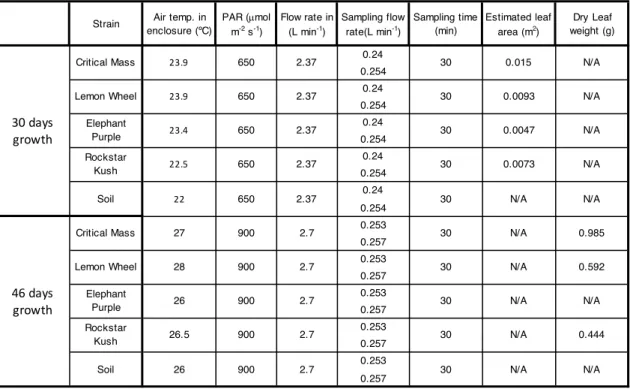
Table 2.1 Summary of leaf enclosure sampling conditions ...24
Table 2.2 The estimated VOC emission rate per plant ...25
Table 2.3 The retention time and fragments of monoterpene ...26
Table 2.4 The terpene emission composition for four different strains ...26
Table 2.5 The estimated Ozone Formation Potential and SOA Formation Potential ...26
Table 3.1 License tiers issued by Colorado Department of Revenue ...58
Table 3.2 The estimated plant count (PC) per cannabis cultivation facility ...58
Table 3.3 Simulation scenarios ...59
Table 3.4 The estimated BVOC and total VOC emission rates ...59
Table 3.5 The process analysis result of nighttime ozone change ...60
Table 3.6 The process analysis result of daytime ozone change ...61
Table 4.1 The summary of experiments... 100
Table 4.2 The details of all samples ... 101
Table 4.3 The GC-MS retention time and fragment ions of explicit monoterpenes ... 102
LIST OF FIGURES
Figure 1.1 The emission of CCFs can impact indoor or outdoor air quality... 4
Figure 2.1 Total terpene emission rate per plant (𝜇g C hr-1) and composition of emissions ... 27
Figure 2.2 Calculated emission capacities (ECs, µgC g-1 hr-1) derived from measurement ... 28
Figure 2.3 The emission capacities for terpene among the three Cannabis spp. strains ... 29
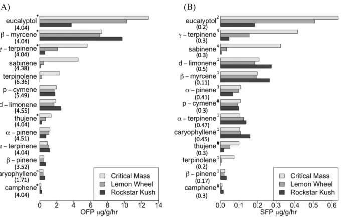
Figure 2.4 The Ozone Formation Potential (OFP)and SOA Formation Potential (SFP)... 30
Figure 3.1 The locations of CCFs and Western Air Quality Model Study domain ... 62
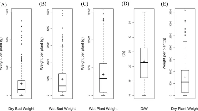
Figure 3.2 The cannabis plant data of Washington state ... 63
Figure 3.3 The maximum increase in TERP concentrations (ppb) for Denver County ... 64
Figure 3.4 The maximum hourly change of TERP across the 4 km ´ 4 km domain ... 65
Figure 3.5 The hourly changes in TERP concentrations ... 66
Figure 3.6 The predicted differences in hourly ozone concentrations ... 67
Figure 3.7 The predicted maximum changes in hourly ozone concentrations ... 67
Figure 3.8 The predicted maximum changes in hourly ozone across 4 km ´ 4 km domain... 68
Figure 3.9 The predicted changes in hourly ozone concentrations for the Denver region ... 69
Figure 3.10 The predicted maximum daily average 8-hour ozone increase ... 69
Figure 3.11 The nighttime case on July 28th, 2011 ... 70
Figure 3.12 The process analysis domain of nighttime ozone change ... 71
Figure 3.13 The process analysis result of nighttime ozone change ... 72
Figure 3.14 The daytime case study on July 18th, 2011 ... 73
Figure 3.15 The process analysis domain for daytime ozone change ... 74
Figure 3.16 The process analysis result for daytime ozone change ... 75
Figure 4.1 The sampling location and Denver map ... 103
Figure 4.2 The observed monoterpene versus the distance to the closest upwind CCF ... 104
Figure 4.3 An isolated CCF experiment ... 105
Figure 4.4 The total and individual terpenoid mixing ratios (pptv) ... 106
Figure 4.5 The 3 hours back-trajectory pathway for all experiments ... 107
Figure 4.6 The monoterpene and terpenoid composition ... 108
Figure 4.7 Monoterpene composition of diurnal experiments 4,5,6 and BG ... 109
LIST OF ABBREVIATIONS AND SYMBOLS
ACOM Atmospheric Chemistry Observations and Modeling Laboratory APCD Air Pollution Control Division
AQCC Air Quality Control Commission
BC base case
BG background
BVOC biogenic volatile organic compounds
CAMx Comprehensive Air Quality Model with Extensions CB6r2 Carbon Bond mechanism 6 reversion 2
CBD Cannabidiol
CCF Cannabis cultivation Facility CDOR Colorado Department of Revenue
CDPHE Colorado Department of Public Health and Environment
CM Critical Mass
DHN decahydronaphthalene
DPW Dry Plant Weight
DRI Dessert Research Institute
EC Emission Capacity
EP Elephant Purple
ER Emission Rate
FID Flame Ionization Detector
GC Gas Chromatograph
IQR Inter Quartile Range IRR Integrated Reaction Rate
IWDW Intermountain West Data Warehouse
LDL Lower Detection Limit
LT Local Time
LW Lemon Wheel
MDA1 maximum daily 1-hour
MDA8 maximum daily 8-hour average
MEGAN Model of Emissions of Gases and Aerosols from Nature MIR Maximum Incremental Reactivity
MS Mass Spectrometer
NAAQS National Ambient Air Quality Standards NCAR National Center for Atmospheric Research
ND non-detected
NEI National Emission Inventory
NIST National Institute of Standards and Technology
NO2 Nitrogen Dioxide
NO3 nitrate radical
NOx nitrogen oxides
NOz NOx termination products
NSF National Science Foundation
NTR organic nitrate
O3 ozone
OFP Ozone Formation Potential
OH hydroxyl radical
PA process analysis
PAR photosynthetically active radiation PBL planetary boundary layer
PC Plant Count
PERMM Python Environment for Reaction Mechanisms/Mathematics
pyPA Python-based Process Analysis
RK Rockstar Kush
RWIS Road/Runway Weather Information System
SFP SOA formation potential
SIP State Implementation Plan SOA secondary organic aerosol
TD Thermal desorption
THC tetrahydrocannabinol
TRO2 total peroxyl radicals
UNGCDP United Nation Global Commission on Drug Policy USEPA United States Environmental Protection Agency VOC volatile organic compounds
CHAPTER 1: INTRODUCTION
As of 2018, 30 states in the U.S. have legalized either medical or recreational Cannabis spp. (marijuana)and national sales have reached 9 billion (Smith, 2018). The earliest two states that legalized recreational cannabis, in 2012, are Washington and Colorado. In Colorado,
recreational business began in 2014 and by 2016 total annual sales reached 1.3 billion dollars. In Colorado, the legalization and commercial production of cannabis has created the establishment of industrial-scale cannabis cultivation facilities (CCFs).
In 2018, there are more than 1 million cannabis plant in Colorado any time. 50% of the cannabis plants and 45% of CCFs are located in Denver County (CDOR, 2019). There are two types of CCF, medical and recreational. The medical usage of cannabis was started in 2009 in Denver County. Those medical cannabis buds include more Cannabidiol (CBD) which is non-psychoactive compound and can be applied for medical usage, such as relieve pain or anti-inflammatory drugs (Nagarkatti et al., 2009; Bonaccorso et al., 2019; Dzierzanowski, 2019). The recreational cannabis usage was started by Colorado state government in 2014. Those
recreational cannabis buds include more tetrahydrocannabinol (THC), which can have the psychological effects (Bonaccorso et al., 2019; Bradford, 2017). Thus, the cannabis plants are high remunerative crop.
plant in indoor environment can be harvested 4-5 times per year, even in winter. Therefore, most of the CCFs in Denver are indoor. Figure 1.1 explains the CCF operation, where previous studies have focused only on the electrical usage (Mills, 2012), waste water, pesticides and fertilizer involved (Bauer et al., 2015). The biogenic volatile organic compounds (BVOC) emissions from marijuana plants, however, have not been assessed for their impact on air quality (Ashworth and Vizuete, 2017).
The Colorado Department of Public Health and Environment (CDPHE) noticed the
cannabis industry cause the environment problems in 2016. The residents complained to CDPHE regarding odour nuisance have soared (Murray, 2016; Rusch, 2016) as the volatile compounds responsible for the characteristic smell of cannabis are released and dispersed from CCF. Some studies indicated that the characteristic odour of Cannabis spp. are responsible by the thiols, the sulfur-containing compounds (Rice and Koziel, 2015b, a). Other studies also indicated that the air quality in CCFs may have the health impact on workers (Jaques et al., 2018; Plautz, 2019). Therefore, the air pollution control division (APCD) in CDPHE conducted the pilot study to qualify and quantify the BVOC concentration in CCF in 2017 (Sakas, 2019), and will report their results in 2020.
from 50-100 ppbv. It is important to note that these concentrations were from illicit growing rooms, containing only hundreds of marijuana plants, which were not under optimal growing conditions. In 2019, the Dessert Research Institute (DRI) reported the monoterpene
concentration in four legal CCFs located in California and Nevada are from 200 ppb-10 ppm (Samburova et al., 2019). Therefore, the current commercially legal CCFs that could lead to potentially larger BVOC emissions. Those BVOCs can become an important VOC source in Denver.
These CCFs grow thousands of marijuana plants in each facility, and have tended to cluster around major highways which offer ease of access for incoming raw materials and to the markets for end products. Highway emissions include nitrogen dioxide and nitric oxide (NOx) that can
interact with the biogenic volatile organic compounds (BVOCs) released from CCFs and potentially impact secondary organic aerosol (SOA) and ozone (O3) concentrations.
Ground-level ozone, is a harmful air pollutant and strong oxidant that is damaging to animal respiratory organs, plants (Heck, 1984), and increases mortality rates (WHO, 2005). Due to ozone’s negative health effects, the United States Environmental Protection Agency (US EPA) has made efforts to control ambient ozone concentrations by establishing the Clean Air Act and National Ambient Air Quality Standards (NAAQS) (USEPA, 2008). Ambient ozone in Denver and Front Range region has been classified with a moderate nonattainment designation by the US EPA (USEPA, 2017b). Previous air quality modeling and analysis from the Western Air Quality Study
regional scale modeling. Once these emission factors are determined, they could then be used in Denver or anywhere this industry is established and growing. Also, there are not ambient
measurement evidences to prove that the CCFs increase the ambient monoterpene concentration in Denver.
Therefore, the goals of this study will, for the first time, use leaf enclosure measurements to quantify BVOC emissions from cannabis plants and calculate their emission factors. In the second part, these emission factors then be applied to estimate the amounts of BVOCs being emitted into the Denver atmosphere. The regulatory model developed by the Colorado for their state implementation plan (SIP) are applied to predict the impacts on ambient ozone
concentrations change in Denver and Front Range. We expect that the increased BVOCs from CCFs will result in spatial and temporal differences of terpene and ozone concentrations. In the last part, we conducted the ambient measurement in Denver near CCF clusters by absorbing cartridges to prove the significant monoterpenes in ambient released from CCF and compared the ambient measurement result with the air quality model result. The result of this study includes the emission factor, ozone impact and ambient measurement, will provide the useful information to help population understand the air quality issue of this new industry, and also help the state government that legalized or plan to start the cannabis industry to access the
REFERENCES
Ashworth, K., and Vizuete, W.: High Time to Assess the Environmental Impacts of Cannabis Cultivation, Environ Sci Technol, 51, 2531-2533, 10.1021/acs.est.6b06343, 2017.
Bauer, S., Olson, J., Cockrill, A., van Hattem, M., Miller, L., Tauzer, M., and Leppig, G.: Impacts of Surface Water Diversions for Marijuana Cultivation on Aquatic Habitat in Four Northwestern California Watersheds, Plos One, 10, 25, 10.1371/journal.pone.0120016, 2015.
Bonaccorso, S., Ricciardi, A., Zangani, C., Chiappini, S., and Schifano, F.: Cannabidiol (CBD) use in psychiatric disorders: A systematic review, Neurotoxicology, 74, 282-298,
10.1016/j.neuro.2019.08.002, 2019.
Bradford, A., What is THC?: https://www.livescience.com/24553-what-is-thc.html, last 2017.
CDOR, C. D. o. R., MED Resources and Statistics:
https://www.colorado.gov/pacific/enforcement/med-resources-and-statistics, last access: 2,
May, 2019, 2019.
Dzierzanowski, T.: Prospects for the Use of Cannabinoids in Oncology and Palliative Care Practice: A Review of the Evidence, Cancers, 11, 17, 10.3390/cancers11020129, 2019.
Fischedick, J. T., Hazekamp, A., Erkelens, T., Choi, Y. H., and Verpoorte, R.: Metabolic fingerprinting of Cannabis sativa L, cannabinoids and terpenoids for chemotaxonomic and drug standardization purposes, Phytochemistry, 71, 2058-2073,
10.1016/j.phytochem.2010.10.001, 2010.
Heck, W. W., Cure, W.W., Rawlings, J.O., Zaragoza, L.J., Heagle, A.S., Heggestad, H.E., Kohut, R.J., Kress, L.W., and Temple, P.J. : Assessing Impacts of Ozone on Agricultural Crops: I. Overview. J. AIr pollut. Control Assoc. 34:729-735, in, 1984.
Hillig, K. W.: A chemotaxonomic analysis of terpenoid variation in Cannabis, Biochem. Syst. Ecol., 32, 875-891, 10.1016/j.bse.2004.04.004, 2004.
Jaques, P. A., Zalay, M., Huang, A., Jee, K., and Schick, S., Measuring Aerisik Particle Emissions from Cannabis Vaporization and Dabbing:
https://no-smoke.org/wp-content/uploads/pdf/2018-Indoor-Air-Cannabis01-Schick.pdf, last 2018.
Martyny, J. W., Serrano, K. A., Schaeffer, J. W., and Van Dyke, M. V.: Potential Exposures Associated with Indoor Marijuana Growing Operations, Journal of Occupational and Environmental Hygiene, 10, 622-639, 10.1080/15459624.2013.831986, 2013.
Mills, E.: The carbon footprint of indoor Cannabis production, Energy Policy, 46, 58-67, 10.1016/j.enpol.2012.03.023, 2012.
Murray, J., The Marijuana Industry’s War on the Poor:
https://www.politico.com/magazine/story/2016/05/what-works-colorado-denver-marijuana-pot-industry-legalization-neighborhoods-dispensaries-negative-213906, last 2016.
Nagarkatti, P., Pandey, R., Rieder, S. A., Hegde, V. L., and Nagarkatti, M.: Cannabinoids as novel anti-inflammatory drugs, Future Med. Chem., 1, 1333-1349, 10.4155/fmc.09.93, 2009.
Plautz, J., As legal pot farms expand, so do air pollution worries:
https://www.sciencemag.org/news/2019/01/legal-pot-farms-expand-so-do-air-pollution-worries, last 2019.
Rice, S., and Koziel, J. A.: The relationship between chemical concentration and odor activity value explains the inconsistency in making a comprehensive surrogate scent training tool representative of illicit drugs, Forensic Sci.Int., 257, 257-270,
10.1016/j.forsciint.2015.08.027, 2015a.
Rice, S., and Koziel, J. A.: Characterizing the Smell of Marijuana by Odor Impact of Volatile Compounds: An Application of Simultaneous Chemical and Sensory Analysis, Plos One, 10, 17, 10.1371/journal.pone.0144160, 2015b.
Rubino, J., Colorado’s average price of a pound of wholesale marijuana grows for fourth straight quarter: https://www.denverpost.com/2019/09/17/colorado-price-wholesale-marijuana/, last access: 2019, 2019.
Rusch, E., Marijuana-infused neighbor conflicts: Ways to clear the air:
Sakas, M. E., Growing Cannabis Could Lead to More Air Pollution:
https://www.sciencefriday.com/segments/cannabis-air-pollution/, last 2019.
Samburova, V., McDaniel, M., Campbell, D., Wolf, M., Stockwell, W. R., and Khlystov, A.: Dominant volatile organic compounds (VOCs) measured at four Cannabis growing facilities: pilot study results, Journal of the Air & Waste Management Association, 1-10, 10.1080/10962247.2019.1654038, 2019.
Smith, A., The U.S. legal marijuana industry is booming:
https://money.cnn.com/2018/01/31/news/marijuana-state-of-the-union/index.html, last 2018.
Turner, C. E., Elsohly, M. A., and Boeren, E. G.: CONSTITUENTS OF CANNABIS-SATIVA L .17. A REVIEW OF THE NATURAL CONSTITUENTS, J. Nat. Prod., 43, 169-234, 10.1021/np50008a001, 1980.
USEPA: National Ambient Air Quality Standards, in, 2008.
USEPA: 8-Hour Ozone (2008) Nonattainment Areas by State/County/Area, in, edited by: USEPA, 2017.
WHO: Air Quality Guidelines for Particulate Matter, Ozone, Nitrogen Dioxide and Sulfur Dioxide-Global Update, World Health Organisation, available at:
https://apps.who.int/iris/bitstream/handle/10665/69477/WHO_SDE_PHE_OEH_06.02_eng.
pdf;jsessionid=07FDCC71EB5AE19425AC18580164DD28?sequence=1 2005.
CHAPTER 2: LEAF ENCLOSURE MEASUREMENTS FOR DETERMINING
VOLATILE ORGANICCOMPOUND EMISSION CAPACITY FROM CANNABIS SPP.1
2.1 Introduction
The use of Cannabis spp. and its various products have long been controversial, with opponents of the relaxation of restrictions pointing to studies linking long-term use to mental health problems (WHO, 2016), and advocates arguing that it provides many therapeutic benefits (Ashton, 2001; Madras, 2015). Supporters of the decriminalization and legalization of Cannabis spp. liken current regulations to the early 20th Century United States prohibition laws, suggesting
that many of the detrimental societal impacts of Cannabisspp. production, sale, and use are directly associated with its illegality. This argument is beginning to hold sway and, for the first time, in 2014, the United Nation Global Commission on Drug Policy (UNGCDP) called for legalization with regulation (UNGCDP, 2014). The UN Office on Drugs and Crime reports over 180 million users worldwide (UNODC, 2016), and the cultivation and use of Cannabisspp. for medical purposes is already legal or decriminalized in more than 40 countries around the world. The UNGCDP argues that regulation of the recreational use of Cannabis spp. would bring transparency at all stages of the supply chain, reducing associated criminal activity and trafficking, ensuring drug safety and allowing monitoring of environmental impacts. Furthermore, legalization of the recreational use of Cannabisspp. offers an opportunity for
1 This chapter previously appeared as an article in the Atmospheric Environment in 2019. The original citation is as
increased fiscal revenue: in the US state of Colorado, tax revenue from sales of Cannabisspp.
for recreational use in 2014 (the first year of legal commercial sales) amounted to over $76 million (UNODC, 2016). Many US states have followed Colorado’s lead, a trend that is expected to spread to many countries around the world.
Cannabis spp. are native to the Indian sub-continent and require warm temperatures and high light intensity to achieve good yields. Optimal growing conditions for commercial varieties are typically around 30 ºC, 1000-1500 µmol m-2 s-1 of photosynthetically active radiation (PAR;
depending on growth stage) and, in an outdoor environment, 22.7 L of water per day per plant (Green, 2009; Mills, 2012; Bauer et al., 2015). Although Cannabis spp. can be grown outdoors in many regions of the world, all large-scale commercial cultivation in Denver, Colorado occurs indoors or in greenhouses. This enables year-round operations, ensures security, and allows for the precise control of the growing environment to maximize yields. At indoor commercial facilities, such as those found in Denver, plants receive light 24 hours per day during the initial growth stages. Since Cannabis spp. are photoperiod sensitive (i.e. only flowering when the length of daylight shortens), once sufficient leafy biomass accumulation has occurred, the lighting regime in these facilities is altered to induce budding. In most cases, a hour on, 12-hour off pattern is used, but this can vary to as little as 8 12-hours on over a 24-12-hour period. Typically, the flower buds are enriched in the active ingredients Tetrahydrocannabinol (THC) and Cannabidiol (CBD) in comparison to foliage, and in most varieties, other plant tissues (stems, branches, roots) contain negligible amounts of these compounds. The average yield of saleable biomass from commercial strains of Cannabis spp. is around 1 kg per plant
The production of Cannabis spp. in indoor facilities has been the focus of studies
quantifying the environmental impacts of energy and water use (Mills, 2012). Considerably less is known about the potential impacts of this industry on indoor and outdoor air quality due to BVOCs emitted directly from the plants themselves. Cannabis spp. plant tissues, such as leaves and buds, are known to contain many BVOCs. Previous studies of dried plant material (Turner et al., 1980; Rice and Koziel, 2015b) and oil extracts from buds (Ross and ElSohly, 1996) have identified high concentrations of monoterpenes (C10H16), other terpenoid compounds (e.g.
eucalyptol; C10H18O), sesquiterpenes (C15H24), and methanol that is associated with plant growth
studies to characterize and specifically quantify the volatile emissions during the growing and budding process. Based on previous studies, however, the Cannabis spp. plantshave the potential to emit VOCs into the facility in which they are grown, and also into the atmosphere.
Emissions of VOCs in urban areas have the potential to contribute to ozone production (Fehsenfeld et al., 1992; Pierce et al., 1998; Ryerson et al., 2001) and the formation of secondary organic aerosol (SOA) (Lee et al., 2006; Kanakidou et al., 2005). Once VOCs are released into the urban atmosphere, they can react with the hydroxyl (OH) radical, nitrate (NO3) radical, and
ozone (O3) (Hites and Turner, 2009; Braure et al., 2014). These initial oxidation reactions lead to
further atmospheric processing, which can ultimately lead to the formation of ozone and SOA. In Denver, for example, where there are >600 Cannabis spp. cultivation facilities releasing BVOCs, the magnitude of these emissions has the potential to impact local and regional air quality,
depending to some extent on the precise mix of compounds emitted. To understand the effect of BVOC emissions from these facilities on atmospheric chemistry and composition, it is necessary to identify and quantify the sources.
The goal of this study was to estimate the emission capacity (EC, µgC g-1 hr-1) range and
terpene emission composition of cannabis plants. There is sparse BVOC data available from enclosure techniques, and thus these studies provide new data on the quantification of emissions of BVOCs from live commercially-available strains of Cannabis spp. at different phenological stages in their lifecycle.
2.2 Methods
compounds and quantify emission rates. The plants were purchased by volunteers and were handled, housed, and sampled in a private off-site location. After the experiments, those plants were disposed of and composted locally. We did not have access to laboratory facilities or a growth room with a controlled environment. Thus, these experiments should be viewed as field measurements.
2.2.1 Cultivation
Four Cannabis spp. strains, commonly found in CCFs in Colorado, were studied: “Rockstar Kush” (RK), “Elephant Purple” (EP), “Lemon Wheel (LW)”, and “Critical Mass” (CM). Twelve plants (3 from each strain) were grown under monitored conditions over a period of 14 weeks during the summer of 2016. The plants were bought on July 8, 2016 and
transplanted to 1 US gallon (3.8 litre) pots on July 15, 2016, at which time one additional pot (used as a control) was filled with identical soil. The soil used was a general use potting soil suitable for most plants. The plants were placed on trays and allowed to acclimate to the growing environment. The plants were kept well-irrigated with water being added to the trays every 2-3 days. In a growing facility growing lights are kept on for 24 hours a day. Thus, three 15W LED growing lamps were positioned 1m above the top of the pots and the growing plants received 500-900 µmol m-2 s-1 of light continuously for 24 hours (dependent on the distances between the
leaf and growth light). The temperature of the growth room was not controlled and ranged between 15 – 30 ºC, which is typical for local ambient conditions during summer in Denver. All plants received the same treatment and were regularly rotated to minimize edge effects and to ensure, as much as possible, that all plants experienced the same light and temperature
2.2.2 Plant Enclosure Sampling
A standard plant enclosure sampling method was applied to measure BVOC emission rates (Tholl et al., 2006; Ortega and Helmig, 2008; Ortega et al., 2008). Air samples were collected from whole-plant enclosures for one specimen of each of the four strains and the blank pot after 12, 30, 46, and 96 days of growth since July 8, 2016. The same sampling routine was followed on each occasion. The pot containing the largest and tallest plant from each strain was selected and placed carefully in a 5 US gallon (19 liters) PFA Teflon pail liner (Welch
Fluorocarbon, Dover, NH, USA). The plants were handled as gently as possible to minimize emissions due to disturbance (Ortega and Helmig, 2008; Ortega et al., 2008).Ambient air was pumped through Teflon tubing (25.4 mm O.D.), first through an activated charcoal filter to remove O3 and VOCs, and then into the enclosure system. This enclosure system was designed
to act as a continuous stirred-tank reactor (CSTR) with a constant flow rate of 2.4-2.7 liter min-1.
A thermocouple was fed into the air space, and the bag was then clamped tightly around the pot until the bag inflated, indicating positive pressure within the enclosure. Since the measurements were done indoors, a 90W growth lamp was positioned above the Teflon bag, delivering 650-900 µmol m-2 s-1 (PAR) at the plant top as measured by a quantum sensor (Li-COR model 190-R,
Lincoln, Nebraska). Air flowed continuously through the enclosure for 30 minutes prior to sampling, allowing time for several exchanges of air and for the VOC concentrations to reach a steady-state. After 30 minutes, BVOC sampling commenced. During sampling, two stainless steel adsorbent cartridges, each containing ~400 mg of Tenax TA and Carbograph 5TD in series (Markes International, Llantrisant, UK), were connected in parallel to the Teflon line exiting the enclosure. Air exiting the enclosure was pulled at a known flow rate (between 220-250 ml min-1)
between 6.5 and 7.5 liters. Terpene concentrations measured in these samples therefore represented an average over that 30-minute collection period, during which time flow rate, irradiance, and air temperature were maintained at a relatively constant value.
Following sampling, each cartridge was securely capped at both ends and refrigerated prior to analysis. After 46 and 96 days of growth, the sampled plants were harvested and dried at room temperature for over one week. At the end of the drying time, leaves and buds were
removed from each plant, and weighed to obtain the dry weight mass (Mdry (g)) for each strain. Of the original 12 plants, the 10 healthiest ones by visual inspection were chosen for sampling. The emission rates were therefore normalized using leaves from the plants that were weighed in the 46- and 96-day growth periods. Details of the leaf enclosure measurements are presented in Table 1. In addition to the enclosure measurements of the four Cannabis spp. strains, air samples were taken from the pot containing only soil and from an otherwise empty enclosure bag to act as controls. For these controls, the soil was moistened, and the Teflon bag was placed around the pot in the same way that the plants were treated.
Enclosure carbon dioxide (CO2) concentrations are important for the calculation of
photosynthesis rates. Further, is important to keep CO2 concentrations similar to ambient
conditions so that BVOC emission rates are not inadvertently affected. These measurements of CO2 concentrations, however, were not available during this study. In the study to keep
concentrations similar to ambient we developed a protocol that set the input air flow rate of 2.4-2.7 L min-1 resulting in a high chamber air exchange rate of 8.2 hr-1. Using this exchange rate we
calculated the reduction in CO2 by assuming: photosynthesis rates of 10 µmol m-2 s-1, ambient
input CO2 concentration of 400 ppm, active leaf area of 0.015 m2 per plant. The estimated
ppm. There amount of reduction is within the normal range of plant enclosure experiments. Therefore, we assume that this did not have an adverse impact on BVOC emission rates. 2.2.3 Analysis method and instrument (GCMS & GCFID)
Samples were thermally desorbed from the cartridges and analysed using a Gas
Chromatograph (GC) (Agilent Technologies, model 7890A) coupled to both a flame ionization detector (FID) and a mass spectrometer (MS) (model 5975C), following published protocols (Harley et al., 2014). Thermal desorption (TD) was achieved by heating the adsorbent cartridges to 275°C in a UNITY TD (model UNITY, Markes International, Llantrisant, UK), followed by focusing the analyses on to a small cryotrap, and then heating this final trap as the analytes were injected on to the column. Helium was used as the carrier gas in the capillary column (RESTEK Rtx-5 model 10224, 30m, 0.32mm, ID, 0.25µm film thickness). The GC oven temperature cycle started at 35°C and was held at that temperature for 1 minute, subsequently increasing 10ºC per minute up to 260ºC for each cartridge. The peak area associated with m/z 93, the dominant monoterpene ion fragment, of each terpenoid was quantified by GC-MS. To account for changes in MS sensitivity, 2ml of an internal standard, decahydronaphthalene (DHN), was sampled on to each adsorbent cartridge during the analysis. The measured terpenoid signals were normalized by dividing the m/z 93 mass fragment by the m/z 95 fragment of DHN. Additional calibrations were performed by loading sorbent tubes with 100 standard cm3 of a gas-phase standard
The National Institute of Standards and Technology (NIST) database was used to identify individual monoterpenes from the GC-MS peaks by their mass fragmentation patterns using electron impact ionization. The preliminary calculations of VOC concentrations based on GC-MS peak areas were cross-checked against the GC-FID. FID peaks of the DHN internal standard were used to ensure consistency and flag instrument drift. The measurement limitations of GC-FID and GC-MS are calculated using the blank sample. For the terpene compounds, the detection limits (DL) are three standard deviations of blank values. The average VOC
concentrations from the two cartridges drawn from each enclosed plant, typically calculated by the GC-FID, was used due to its stability and linearity. In the case that there was a co-elution effect and the FID signal was lower than the FID detection limits, the GC-MS results were used. The DL of terpene by GC-MS is 0.004 µg C hr-1. If the results were lower than the limits a
Non-Detection symbol (ND) is shown. All of the emission rate calculated from the FID and MS signal are included in the supplemental document as Table 2.2(A) and Table 2.2(B). Other details about the analysis, such as retention time of each terpene species and fragment percentage of ion m/z
93 are also included in the supplemental document shown in Table 2.3. 2.2.4 Calculation of Emission Capacity
The EC and its algorithms were standardized in Guenther et al., 1993 and are based entirely on temperature and incident light energy.Our study follows these best practices, which
have been applied to several studies (Sakulyanontvittaya et al., 2008; Funk et al., 2003; Ortega
and Helmig, 2008; Ortega et al., 2008). While this is the standard practice in derivation of EC for atmospheric chemistry-climate modelling, there is evidence to suggest that monoterpene
share a common synthesis pathway with isoprene, direct emissions of certain monoterpenes are dependent on light as well as temperature (Kesselmeier and Staudt, 1999; Lichtenthaler, 1999). In absence of direct evidence, such as that provided by light-dark transition experiments, the light-independent (Tingey et al., 1980; Guenther et al., 1991) and light-dependent algorithms (Guenther et al., 1993; Staudt et al., 1997; Guenther, 1997) were both therefore calculated for the potential EC of all terpenoid emissions.
Based on the concentration of each VOC calculated by GC-MS/FID and the air sampling flow rate, a rate of emission, Fi(µgC g-1 h-1), for each VOC species i was calculatedusing Equation 2.1 (Ortega and Helmig, 2008):
𝐹# =%&'()*+1,'(-./+0&
230 (2.1)
where 𝐶#567 is the concentration of VOC species i (µgC mol-1) in air exiting the enclosure
containing a Cannabis spp. plant, 𝐶#89:7; is the concentration of VOC species i (µgC mol-1) in
air exiting the enclosure containing only the empty pot with soil and water, 𝑀=>; is the dry mass of leaves (g), and 𝑄 is the flow rate of air into the enclosure system (about 5.44 mol h-1).
Calculated values of Fi therefore represent emission rates at measured temperatures and PAR. The emission capacity (ei) for VOC i was calculated following Guenther et al. (1995) :
𝜀# = 𝐹#/𝛾 (2.2)
where ei is the emission capacity at 𝑇D=30 ºC (µgC g-1 h-1), Fi is the emission rate of the VOC i
(µgC g (dry matter)-1 h-1) calculated using Equation 2.1, and g is a dimensionless activity factor
which corrects for temperature and light conditions. In equation 2.3, g is defined for temperature and independent of light.
where b is an empirical coefficient (in K-1) taken as b=0.09 for all monoterpenes, eucalyptol, and
sesquiterpenes (Guenther et al., 1991; Ortega and Helmig, 2008; Ortega et al., 2008).
In equation 2.4, the g is a factor with a light dependent condition(Guenther et al., 1993; Guenther, 1997; Staudt et al., 1997).
𝛾 = N O'PQR
√TUOVRVW X
8Y:Z[\Q(\]\^) _\^\ ` '\aU8Y:b[\Vc\]\de_\^\ f
g (2.4)
where L is the photosynthetically active radiation (PAR, µmol m-2 s-1 ), R is the ideal gas
constant (8.314J.K-1mol-1). a(=0.0027), C
L1 (=1.066), CT1 (=95,000 J mol-1), CT2 (=230,000 J
mol-1), C
T3 (=0.961) and TM (=41 ºC) are empirical coefficients.
2.3 Results
The terpene emission rates per plant (µgC h-1) and the percentage composition of the
different emitted terpenes were calculated at 30 and 46 days of growth for all four Cannabis spp.
µgC h-1 and 8.6 µgC h-1 per plant. The terpenoid composition of Critical Mass emissions also
changed across the different growth stages, at 30 days of growth the terpenoids with the highest emission rates were β-myrcene (43%), and eucalyptol (19%). Sixteen days later the largest emitted species were eucalyptol (32%), β-myrcene (18%) and γ-terpinene (14%). For Lemon Wheel, eucalyptol (33%, 38%) and β-myrcene (26%, 27%) were the dominant emissions. For Elephant Purple and Rockstar Kush the highest emissions were from β-myrcene (39% and 41%), eucalyptol (25% and 28%), and d-limonene (17% and 8%) at 30 days. At 46 days Elephant Purple and Rockstar Kush had increases in γ-terpinene (8%) and caryophyllene (5%) emissions.
After 46 days of growth, the ECs of three different strains were calculated at 30 ºC and normalized by dry leaf weight (Figure 2.2A). These were calculated using GC-FID data unless there was a co-elution effect and the GC-MS signal was used as shown in Table 2.4. Dry leaf mass was not measured for Elephant Purple, hence EC could not be calculated for this strain. The highest total terpene EC (including monoterpenes, eucalyptol and caryophyllene) was 8.7±0.7 µgC g-1 hr-1 for the Critical Mass strain, of which 5.7±0.5 µgC g-1 hr-1 (66%) was monoterpenes,
2.8±0.19 µgC g-1 hr-1 (32%) was eucalyptol, and 0.2±0.01 µgC g-1 hr-1 (2%) was caryophyllene.
Total terpene EC for Lemon Wheel and Rockstar Kush were 5.9 µgC g-1 hr-1 and 4.9 µgC g-1 hr -1. For Lemon Wheel, eucalyptol contributed 2.2 µgC g-1 hr-1 (38%) and monoterpenes 3.5 µgC g -1 hr-1 (59%); whereas for Rockstar Kush, the contributions were 0.8 µgC g-1 hr-1 (17%)and 3.7
µgC g-1 hr-1 (76%). The complete emission capacities of all terpene species, based using both the
GC-FID and GC-MS data, are shown for all strains in Figure 2.3.
The emission variations of each terpene species among the three different Cannabis spp.
are monoterpenes (ranging between 3.1-5.5 µgC g-1 hr-1) and eucalyptol (1.0-3.0 µgC g-1 hr-1).
The absolute value and range of caryophyllene emission capacities are much smaller at 0.18-0.3 µgC g-1 hr-1.
To understand the potential impact of these emissions on air quality, the Ozone
Formation Potential (OFP) in μg ozone per gram dry weight of Cannabis spp. per hour of each terpene was calculated as shown in Equation 2.5 (Ou et al., 2015) :
OFP = Emission capacity (μg/g/hr) × MIR (ozone(g)/VOC(g)) (2.5)
where MIR is the Maximum Incremental Reactivity (CARB, 2010) defined as the maximum number of grams of ozone produced per gram of reactant VOC. For this study, if a specific MIR is not available, the reported average monoterpene MIR (4.04 ozone(g)/VOC(g)) was applied to calculate OFPs. A surrogate MIR for a C15 alkene was used for caryophyllene, due to it having the same carbon number and being a similar alkene species.
Figure 2.4(A) shows the OFP estimated for the individual terpenes emitted from three
Cannabis spp. strains (Critical Mass, Lemon Wheel, and Rockstar Kush). The total OFP rate of Critical Mass is 41 µg g-1 hr-1, Lemon Wheel is 27 µg g-1 hr-1 and Rockstar Kush is 22 µg g-1 hr-1.
For Critical Mass and Lemon Wheel, the eucalyptol and β-myrcene species make up 50% of the total OFP rate. The OFPs of Critical Mass for eucalyptol and β-myrcene are 12.8 µg g-1 hr-1 and
7.3 µg g-1 hr-1. The OFPs of Lemon Wheel for eucalyptol and β-myrcene are 10.2 µg g-1 hr-1 and
7.1 µg g-1 hr-1. Rockstar Kush has a higher β-myrcene OFP rate, which is 9.7 µg g-1 hr-1, and
Figure 2.4(B) shows the SOA formation potentials (SFPs) based on the (SOA) yield (Iinuma et al., 2009; Lee et al., 2006; Fry et al., 2014; Slade et al., 2017) of individual terpenes as calculate from Equation 2.6.
SFP = Emission capacity (μg/g/hr) × SOA Yield (2.6)
Figure 2.4(B) estimated the SOA formation potential from the terpene species emitted from Critical Mass, Lemon Wheel and Rockstar Kush after 46 days of growth. For compounds without a published SOA yield (marked: #), we assumed an SOA yield 0.3. The total SFP of Critical Mass is about 2.4 µg g-1 hr-1; with eucalyptol generating 0.63µg g-1 hr-1 of SOA, and
γ-terpinene 0.4 µg g-1 hr-1 of SOA. For Lemon Wheel, the total SFP is 1.6 µg g-1 hr-1, with
eucalyptol contributing 0.51 µg g-1 hr-1, β-myrcene is 0.19 µg g-1 hr-1 and d-limonene is 0.19 µg
g-1 hr-1. For Rockstar Kush, the total SFP is 1.3 µg g-1 hr-1, with 0.26 µg g-1 hr-1 from β-myrcene,
and 0.27 µg g-1 hr-1 from d-limonene. Eucalyptol, γ-terpinene, and d-limonene have the largest
SOA yields, but emissions were low for the strains tested here. The complete numbers of OFP and SFP of all terpenes for all strains are in supplemental Table 2.5.
2.4 Discussion and Conclusion
α-pinene and β-α-pinene being the dominant terpene emissions with comparable amounts of 2
-methyl-3-buten-2-ol (Harley et al., 1998). Terpene emissions from all our Cannabis spp. strains had eucalyptol and 𝛽-myrcene as the highest emitted species. Ross et al. (Ross and ElSohly, 1996) also found that fresh buds of Cannabis spp. plants were about 67% β-myrcene. Similar to our results, Fischedick et al. 2010 (Fischedick et al., 2010) found that terpenes extracted from buds had different compositions across 11 strains. In six of these strains the dominant terpene was also β-myrcene (>35%).
It is important to note that for large-scale Cannabis spp. cultivation facilities the growth conditions are optimized. This includes elevating CO2 concentrations to 1,500 ppm in growing
rooms, carefully managing water use, elevating light to >1,000 µmol m-2 s-1 (PAR), and
would enable authorities to assess the potential impacts of this new industry on regional air quality and if necessary determine mitigation strategies.
According to the Colorado Department of Revenue (CDOR, 2018a), there were more than 1,400 CCFs in Colorado in 2017, with over 600 in the Denver metro area. If these emissions from these cultivations are released into the ambient atmosphere they have the potential to impact local ozone and particulate matter (PM). For example, if each of the 600 facilities in Denver contained the permitted 10,000 plants (CDOR, 2018a), with an assumed biomass of 1 kg/plant (Jankauskiene and Gruzdeviene, 2015; Green, 2009), and all emissions were released into the atmosphere, a EC of 8.7 µgC g-1 hr-1 emission capacity would result in the annual total
terpene emission of 520 metric ton year-1. This emission rate is more than twice that of the 250
metric ton year-1 of total biogenic VOC emissions for Denver as estimated by the Western Air
Quality Study (WAQS, 2017) for Colorado’s 2008 regulatory air quality model simulations (RAQC, 2016). Using MIR values shown in Figure 2.4 these BVOC emissions could produce 2,100 metric ton year-1 of ozone, and using the yields shown in Figure 2.4 produce 131 metric
ton year-1 of PM. Given the location of the VOCs emitted from Cannabis spp. from facilities in
downtown Denver near major urban anthropogenic sources, there is the potential for the
Table 2.1 Summary of leaf enclosure sampling conditions including flow rates, leaf area (when measured), and dry leaf weight.
Strain Air temp. in enclosure (ºC)
PAR (µmol m-2 s-1)
Flow rate in (L min-1)
Sampling flow rate(L min-1)
Sampling time (min)
Estimated leaf area (m2)
Dry Leaf weight (g) 0.24 0.254 0.24 0.254 0.24 0.254 0.24 0.254 0.24 0.254 0.253 0.257 0.253 0.257 0.253 0.257 0.253 0.257 0.253 0.257 2.7 2.7 2.7 2.7 2.7 2.37 2.37 2.37 2.37 2.37 30 0.0073
Soil 22 650
26.5 900 30 N/A
Soil
30 days growth
Critical Mass 23.9 650 30 0.015
Lemon Wheel 23.9 650 30 0.0093
Elephant
Purple 23.4 650 30 0.0047
Rockstar
Kush 22.5 650
N/A
26 900 30 N/A
30 N/A
46 days growth
Critical Mass 27 900 30 N/A
Lemon Wheel 28 900 30 N/A
Elephant
Purple 26 900 30 N/A
Table 2.2 The estimated VOC emission rate per plant (µgC h-1) based on data from the Gas
Chromatograph coupled to a flame ionization detector FID) and mass spectrometer (GC-MS) (A) without a light dependency and (B) with a light dependency. The bold font indicates the data used to estimate emission capacity (EC). When possible the GC-FID data was selected due to its stability and linearity. If there was a co-elution effect, or if the GC-FID signal was lower than the detection limits, then the GC-MS results were used.
(A)
(B)
Strains Terpene thujene alpha-pinene camphene sabinene beta-pinene beta-myrcenephellandrenealpha- terpinenealpha- p-cymene d-limonene cis-beta-ocimene terpinenegamma- terpinolene caryophyllene eucalyptol FID ( µg C / h) 0.033 0.060 0.037 0.024 0.096 0.592 - - 0.048 0.077 0.039 0.044 ND 0.021 0.258
MS (µg C / h) 0.050 0.060 0.015 0.027 0.029 0.467 0.012 0.028 - 0.112 0.049 0.071 0.021 - -FID ( µg C / h) 0.029 0.031 0.034 - - 0.243 ND - 0.021 0.040 ND 0.088 ND ND 0.300
MS (µg C / h) 0.039 0.028 0.007 0.046 0.036 0.073 ND 0.014 - 0.058 0.012 0.079 0.021 - -FID ( µg C / h) ND ND ND ND ND 0.364 ND ND 0.120 0.162 ND ND ND ND 0.237
MS (µg C / h) 0.008 0.008 ND ND ND 0.116 ND ND - 0.025 0.021 0.019 ND - -FID ( µg C / h) 0.013 0.009 0.031 ND ND 0.291 ND ND 0.018 0.057 ND ND ND ND 0.195
MS (µg C / h) 0.010 0.007 0.017 ND ND 0.164 ND ND - 0.046 0.042 0.043 ND -
-FID ( µg C / h) ND ND ND ND ND ND ND ND ND ND ND ND ND ND ND
MS (µg C / h) ND ND ND ND ND ND ND ND ND ND ND ND ND ND ND
FID ( µg C / h) 0.291 0.232 - 0.939 - 1.573 - 0.195 0.312 0.363 ND 1.203 0.324 0.202 2.751
MS (µg C / h) 0.318 0.278 0.028 0.260 0.123 1.164 0.055 0.132 - 0.237 ND 0.452 0.127 - -FID ( µg C / h) 0.090 0.126 - 0.062 - 0.917 - 0.139 0.163 0.194 ND 0.271 ND 0.125 1.324
MS (µg C / h) 0.084 0.127 0.009 0.060 0.063 0.264 0.019 0.043 - 0.162 ND 0.150 0.022 - -FID ( µg C / h) 0.076 0.131 ND ND - 2.663 - - 0.028 0.136 ND 0.356 ND 0.222 0.759
MS (µg C / h) 0.066 0.109 ND 0.010 0.060 1.592 0.016 0.024 - 0.199 ND 0.138 ND - -FID ( µg C / h) 0.026 0.065 - ND - 0.942 ND 0.116 0.128 0.215 ND - ND 0.139 0.362
MS (µg C / h) 0.013 0.063 0.022 0.007 0.076 0.585 ND 0.024 - 0.162 ND 0.060 ND -
-FID ( µg C / h) ND ND ND ND ND ND ND ND ND ND ND ND ND ND ND
MS (µg C / h) ND ND ND ND ND ND ND ND ND ND ND ND ND ND ND
46 days of growth Critical Mass Lemon Wheel Elephant Purple Rockstar Kush
Blank pot with soil 30 days of growth Critical Mass Lemon Wheel Elephant Purple Rockstar Kush
Blank pot with soil
Strains Terpene thujene alpha-pinene camphene sabinene beta-pinenebeta-myrcene alpha-phellandren
e
alpha-terpinene p-cymene d-limonene cis-beta-ocimene terpinenegamma- terpinolene caryophyllene eucalyptol
FID ( µg C / h) 0.043 0.077 0.047 0.031 0.124 0.760 - - 0.062 0.099 0.050 0.057 ND 0.028 0.331
MS (µg C / h) 0.032 0.039 0.010 0.017 0.019 0.299 0.008 0.018 - 0.072 0.031 0.046 0.013 - -FID ( µg C / h) 0.037 0.040 0.043 - - 0.311 ND - 0.028 0.051 ND 0.113 ND ND 0.385
MS (µg C / h) 0.025 0.018 0.005 0.029 0.023 0.047 ND 0.009 - 0.037 0.008 0.051 0.013 -
-FID ( µg C / h) ND ND ND ND ND 0.476 ND ND 0.157 0.211 ND ND ND ND 0.310
MS (µg C / h) 0.005 0.005 ND ND ND 0.076 ND ND - 0.016 0.013 0.012 ND -
-FID ( µg C / h) 0.016 0.017 0.042 ND ND 0.395 ND ND 0.024 0.077 ND ND ND ND 0.263
MS (µg C / h) 0.007 0.005 0.012 ND ND 0.111 ND ND - 0.031 0.028 0.029 ND -
-FID ( µg C / h) ND ND ND ND ND ND ND ND ND ND ND ND ND ND ND
MS (µg C / h) ND ND ND ND ND ND ND ND ND ND ND ND ND ND ND
FID ( µg C / h) 0.314 0.250 - 1.015 - 1.699 - 0.211 0.337 0.392 ND 1.299 0.350 0.218 2.893
MS (µg C / h) 0.343 0.300 0.030 0.281 0.133 1.257 0.060 0.143 - 0.256 ND 0.488 0.121 - -FID ( µg C / h) 0.094 0.132 - 0.065 - 0.961 - 0.146 0.171 0.203 ND 0.283 ND 0.135 1.387
MS (µg C / h) 0.088 0.133 0.009 0.063 0.066 0.276 0.020 0.045 - 0.169 ND 0.157 0.023 - -FID ( µg C / h) 0.085 0.146 ND ND - 2.974 - - 0.031 0.152 ND 0.398 ND 0.248 0.847
MS (µg C / h) 0.074 0.122 ND 0.011 0.066 1.778 0.018 0.027 - 0.222 ND 0.155 ND - -FID ( µg C / h) 0.028 0.071 - ND - 1.034 ND 0.127 0.141 0.237 ND - ND 0.153 0.397
MS (µg C / h) 0.014 0.069 0.024 0.008 0.084 0.642 ND ND - 0.178 ND 0.066 ND -
-FID ( µg C / h) ND ND ND ND ND ND ND ND ND ND ND ND ND ND ND
MS (µg C / h) ND ND ND ND ND ND ND ND ND ND ND ND ND ND ND
46 days of growth Critical Mass Lemon Wheel Elephant Purple Rockstar Kush
Blank pot with soil 30 days of growth Critical Mass Lemon Wheel Elephant Purple Rockstar Kush
Table 2.3 The retention time and fragment used for Gas Chromatograph with mass spectrometer (GC-MS)
Table 2.4 The terpene emission composition for four different strains
Table 2.5 The estimated Ozone Formation Potential (OFP) and SOA Formation Potential (SFP) for all observed terpenes.
Terpene time (min)Retention fragment used for quantitation
m/z 93 fragment(%)
thujene 8.4 93 28.6
alpha-pinene 8.56 93 26.3
camphene 8.89 93 18.8
sabinene 9.3 93 26.6
beta-pinene 9.43 93 25.5
beta-myrcene 9.54 93 23.7
alpha-phellandrene 9.93 93 32.1
alpha-terpinene 10.13 93 15.4
p-cymene 10.28 119
-d-limonene 10.39 93 12
cis-beta-ocimene 10.56 93 22.4
gamma-terpinene 10.87 93 20
terpinolene 11.38 121 14.5
caryophyllene 16.9 93
-eucalyptol 10.5 93
-emission rate
(µg C / h) thujene alpha-pinene camphene sabinene beta-pinene beta-myrcene
alpha-phellandrene terpinenealpha- p-cymene d-limonene cis-beta-ocimene terpinenegamma- terpinolene caryophyllene eucalyptol Critical Mass 1.392 2.4% 4.3% 2.6% 1.7% 6.9% 42.6% 0.9% 2.0% 3.4% 5.5% 2.8% 3.2% 1.5% 1.5% 18.5% Lemon Wheel 0.913 3.1% 3.4% 3.7% 5.0% 3.9% 26.6% 0.0% 1.5% 2.3% 4.4% 1.3% 9.7% 2.3% 0.0% 32.8% Elephant Purple 0.942 0.9% 0.8% 0.0% 0.0% 0.4% 38.6% 0.0% 0.0% 12.8% 17.2% 2.2% 2.0% 0.0% 0.0% 25.1% Rockstar Kush 0.703 1.8% 1.3% 4.4% 0.0% 0.5% 41.5% 0.0% 0.0% 2.6% 8.1% 5.9% 6.2% 0.0% 0.0% 27.7% Critical Mass 8.589 3.4% 2.7% 0.3% 10.9% 1.4% 18.3% 0.6% 2.3% 3.6% 4.2% 0.0% 14.0% 3.8% 2.4% 32.0% Lemon Wheel 3.521 2.6% 3.6% 0.3% 1.7% 1.8% 26.0% 0.5% 3.9% 4.6% 5.5% 0.0% 7.7% 0.6% 3.6% 37.6% Elephant Purple 4.480 1.7% 2.9% 0.0% 0.2% 1.3% 59.4% 0.4% 0.5% 0.6% 3.0% 0.0% 8.0% 0.0% 5.0% 16.9% Rockstar Kush 2.157 1.2% 3.0% 1.0% 0.3% 3.5% 43.7% 0.0% 5.4% 6.0% 10.0% 0.0% 2.8% 0.0% 6.4% 16.8% 30 days of growth 40 days of growth
OFP (µg/g/h) thujene
alpha-pinene camphene sabinene beta-pinene beta-myrcene
alpha-terpinene p-cymene d-limonene
gamma-terpinene terpinolene caryophyllene eucalyptol
Critical Mass 1.4 1.2 0.1 4.5 0.5 7.3 0.9 2.0 1.9 5.6 2.4 0.4 12.8
Lemon Wheel 0.7 1.1 0.1 0.5 0.4 7.1 1.1 1.7 1.7 2.1 0.3 0.4 10.2
Rockstar Kush 0.3 0.7 0.2 0.1 0.7 9.7 1.2 1.8 2.5 0.6 0.0 0.6 3.7
SFP (µg/g/h)
Critical Mass 0.10 0.11 0.01 0.32 0.02 0.20 0.11 0.11 0.21 0.42 0.07 0.10 0.63
Lemon Wheel 0.05 0.10 0.01 0.03 0.02 0.19 0.13 0.09 0.19 0.16 0.01 0.11 0.51
Figure 2.1 Total terpene emission rate per plant (𝜇g C hr-1) and composition of emissions for (A) 30-day, and (B) 46-day growth periods from four strains of Cannabis spp.: Critical Mass, Lemon wheel, Elephant Purple, and Rockstar Kush. Numbers in parentheses represent the percentage of total emissions.
Figure 2.2 Calculated emission capacities (ECs, µgC g-1 hr-1) derived from measurements after
46 days of growth normalized by dry leaf weight (g) and a standard temperature of 30ºC for (A) Critical Mass, Lemon Wheel, and Rockstar Kush strains of Cannabis spp., and the variation of EC for (B) total monoterpenes, eucalyptol and caryophyllene among the three strains. No EC for the Elephant Purple strain was estimated due to lack of dry leaf mass data. Eucalyptol is a cyclic ether with a terpenoid structure (C10H18O), the monoterpene structure is C10H16, and
caryophyllene is C15H24.
Figure 2.3 The emission capacities for all measured terpene compounds among the three
Cannabis spp. strains. cis−β−ocimene
camphene α−phellandrene
β−pinene
α−terpinene caryophyllene α−pinene thujene p−cymene terpinolene d−limonene
sabinene γ−terpinene
β−myrcene
eucalyptol
0.0 0.5 1.0 1.5 2.0 2.5 3.0
Figure 2.4 For the Critical Mass, Lemon Wheel, and Rockstar Kush strains, after 46 days of growth, the (A) The Ozone Formation Potential (OFP) rate estimated using the Maximum Incremental Reactivity (MIR) ratio (CARB, 2010) and (B) estimated SOA Formation Potential (SFP) based on published SOA yields [1(Lee et al., 2006), 2(Iinuma et al., 2009), 3(Slade et al.,
2017), and 4(Fry et al., 2014)]. * Used monoterpene MIR = 4.04 ´ Used 15C-alkene MIR = 1.71
# compounds without a published SOA yield, assumed to be 0.3
REFERENCES
Ashton, C. H.: Pharmacology and effects of cannabis: a brief review, Br. J. Psychiatry, 178, 101-106, 10.1192/bjp.178.2.101, 2001.
Ashworth, K., and Vizuete, W.: High Time to Assess the Environmental Impacts of Cannabis Cultivation, Environ Sci Technol, 51, 2531-2533, 10.1021/acs.est.6b06343, 2017.
Bauer, S., Olson, J., Cockrill, A., van Hattem, M., Miller, L., Tauzer, M., and Leppig, G.: Impacts of Surface Water Diversions for Marijuana Cultivation on Aquatic Habitat in Four Northwestern California Watersheds, Plos One, 10, 25,
10.1371/journal.pone.0120016, 2015.
Bonaccorso, S., Ricciardi, A., Zangani, C., Chiappini, S., and Schifano, F.: Cannabidiol (CBD) use in psychiatric disorders: A systematic review, Neurotoxicology, 74, 282-298, 10.1016/j.neuro.2019.08.002, 2019.
Bradford, A., What is THC?: https://www.livescience.com/24553-what-is-thc.html, last 2017.
Braure, T., Bedjanian, Y., Romanias, M. N., Morin, J., Riffault, V., Tomas, A., and Coddeville, P.: Experimental Study of the Reactions of Limonene with OH and OD Radicals: Kinetics and Products, J. Phys. Chem. A, 118, 9482-9490, 10.1021/jp507180g, 2014.
CARB, C. A. R. B., FINAL regulation order Tables of Maximum Incremental Reactivity (MIR) Values: https://www.arb.ca.gov/consprod/regs/2012/4mirtable50411.pdf, last 2010.
CDOR, Licensees - Marijuana Enforcement Division:
https://www.colorado.gov/pacific/enforcement/med-licensed-facilities, last access: 2
May, 2019, 2018.
CDOR, C. D. o. R., MED Resources and Statistics:
https://www.colorado.gov/pacific/enforcement/med-resources-and-statistics, last access:
2, May, 2019, 2019.
Fehsenfeld, F., Calvert, J., Fall, R., Goldan, P., Guenther, A. B., Hewitt, C. N., Lamb, B., Liu, S., Trainer, M., Westberg, H., and Zimmerman, P.: EMISSIONS OF VOLATILE
ORGANIC COMPOUNDS FROM VEGETATION AND THE IMPLICATIONS FOR ATMOSPHERIC CHEMISTRY, Glob. Biogeochem. Cycle, 6, 389-430,
10.1029/91gb02965, 1992.
Fischedick, J. T., Hazekamp, A., Erkelens, T., Choi, Y. H., and Verpoorte, R.: Metabolic fingerprinting of Cannabis sativa L, cannabinoids and terpenoids for chemotaxonomic and drug standardization purposes, Phytochemistry, 71, 2058-2073,
10.1016/j.phytochem.2010.10.001, 2010.
Fry, J. L., Draper, D. C., Barsanti, K. C., Smith, J. N., Ortega, J., Winkler, P. M., Lawler, M. J., Brown, S. S., Edwards, P. M., Cohen, R. C., and Lee, L.: Secondary organic aerosol formation and organic nitrate yield from NO3 oxidation of biogenic hydrocarbons, Environ Sci Technol, 48, 11944-11953, 10.1021/es502204x, 2014.
Funk, J. L., Jones, C. G., Baker, C. J., Fuller, H. M., Giardina, C. P., and Lerdau, M. T.: Diurnal variation in the basal emission rate of isoprene, Ecol. Appl., 13, 269-278, 10.1890/1051-0761(2003)013[0269:dvitbe]2.0.co;2, 2003.
Green, G.: Cannabis Grow Bible: The Definitive Guide to Growing Marijuana for Recreational and Medical Use., 2009.
Guenther, A., Monson, R. K., and Fall, R.: ISOPRENE AND MONOTERPENE EMISSION RATE VARIABILITY - OBSERVATIONS WITH EUCALYPTUS AND EMISSION RATE ALGORITHM DEVELOPMENT, Journal of Geophysical
Research-Atmospheres, 96, 10799-10808, 10.1029/91jd00960, 1991.
Guenther, A., Zimmerman, P. R., Harley, P. C., Monson, R. K., and Fall, R.: ISOPRENE AND MONOTERPENE EMISSION RATE VARIABILITY - MODEL EVALUATIONS AND SENSITIVITY ANALYSES, Journal of Geophysical Research-Atmospheres, 98, 12609-12617, 10.1029/93jd00527, 1993.
Guenther, A.: Seasonal and spatial variations in natural volatile organic compound emissions, Ecol. Appl., 7, 34-45, 10.2307/2269405, 1997.
Harley, P., Fridd-Stroud, V., Greenberg, J., Guenther, A., and Vasconcellos, P.: Emission of 2-methyl-3-buten-2-ol by pines: A potentially large natural source of reactive carbon to the atmosphere, Journal of Geophysical Research-Atmospheres, 103, 25479-25486,
Harley, P., Eller, A., Guenther, A., and Monson, R. K.: Observations and models of emissions of volatile terpenoid compounds from needles of ponderosa pine trees growing in situ: control by light, temperature and stomatal conductance, Oecologia, 176, 35-55, 10.1007/s00442-014-3008-5, 2014.
Heck, W. W., Cure, W.W., Rawlings, J.O., Zaragoza, L.J., Heagle, A.S., Heggestad, H.E., Kohut, R.J., Kress, L.W., and Temple, P.J. : Assessing Impacts of Ozone on Agricultural Crops: I. Overview. J. AIr pollut. Control Assoc. 34:729-735, in, 1984.
Hillig, K. W.: A chemotaxonomic analysis of terpenoid variation in Cannabis, Biochem. Syst. Ecol., 32, 875-891, 10.1016/j.bse.2004.04.004, 2004.
Hites, R. A., and Turner, A. M.: Rate Constants for the Gas-Phase beta-Myrcene plus OH and Isoprene plus OH Reactions as a Function of Temperature, International Journal of Chemical Kinetics, 41, 407-413, 10.1002/kin.20413, 2009.
Hood, L. V. S., Dames, M. E., and Barry, G. T.: Headspace Volatiles of Marijuana, Nature, 1973.
Hood, L. V. S. D., M. E.; Barry, G. T. : Headspace Volatiles of Marijuana, Nature, 1973.
Iinuma, Y., Boge, O., Keywood, M., Gnauk, T., and Herrmann, H.: Diaterebic Acid Acetate and Diaterpenylic Acid Acetate: Atmospheric Tracers for Secondary Organic Aerosol
Formation from 1,8-Cineole Oxidation, Environmental Science & Technology, 43, 280-285, 10.1021/es802141v, 2009.
Jankauskiene, Z., and Gruzdeviene, E.: Screening of Industrial Hemp (Cannabis sativa L.) Cultivars for Biomass Yielding Capacities in Lithuania, J. Nat. Fibers, 12, 368-377, 10.1080/15440478.2014.929556, 2015.
Jaques, P. A., Zalay, M., Huang, A., Jee, K., and Schick, S., Measuring Aerisik Particle Emissions from Cannabis Vaporization and Dabbing:
https://no-smoke.org/wp-content/uploads/pdf/2018-Indoor-Air-Cannabis01-Schick.pdf, last 2018.
Kesselmeier, J., and Staudt, M.: Biogenic volatile organic compounds (VOC): An overview on emission, physiology and ecology, J. Atmos. Chem., 33, 23-88,
10.1023/a:1006127516791, 1999.
Leafly, Cannabis Strain Explorer: https://www.leafly.com/explore/sort-alpha, last access: 2 May, 2019, 2018.
Lee, A., Goldstein, A. H., Keywood, M. D., Gao, S., Varutbangkul, V., Bahreini, R., Ng, N. L., Flagan, R. C., and Seinfeld, J. H.: Gas-phase products and secondary aerosol yields from the ozonolysis of ten different terpenes, Journal of Geophysical Research-Atmospheres, 111, 18, 10.1029/2005jd006437, 2006.
Lichtenthaler, H. K.: The 1-deoxy-D-xylulose-5-phosphate pathway of isoprenoid biosynthesis in plants, Annu. Rev. Plant Physiol. Plant Molec. Biol., 50, 47-65,
10.1146/annurev.arplant.50.1.47, 1999.
Madras, B. K.: Update of Cannabis and its Medical Use, World Health Organisation, available
at: http://www.who.int/medicines/access/controlled-substances/6_2_cannabis_update.pdf
2015.
Marchini, M., Charvoz, C., Dujourdy, L., Baldovini, N., and Filippi, J. J.: Multidimensional analysis of cannabis volatile constituents: Identification of 5,5-dimethyl-1-vinylbicyclo 2.1.1 hexane as a volatile marker of hashish, the resin of Cannabis sativa L, J.
Chromatogr. A, 1370, 200-215, 10.1016/j.chroma.2014.10.045, 2014.
Martyny, J. W., Serrano, K. A., Schaeffer, J. W., and Van Dyke, M. V.: Potential Exposures Associated with Indoor Marijuana Growing Operations, Journal of Occupational and Environmental Hygiene, 10, 622-639, 10.1080/15459624.2013.831986, 2013.
Mills, E.: The carbon footprint of indoor Cannabis production, Energy Policy, 46, 58-67, 10.1016/j.enpol.2012.03.023, 2012.
Murray, J., The Marijuana Industry’s War on the Poor:
https://www.politico.com/magazine/story/2016/05/what-works-colorado-denver-marijuana-pot-industry-legalization-neighborhoods-dispensaries-negative-213906, last
2016.
Niinemets, U., Loreto, F., and Reichstein, M.: Physiological and physicochemical controls on foliar volatile organic compound emissions, Trends Plant Sci, 9, 180-186,
10.1016/j.tplants.2004.02.006, 2004.
Ortega, J., and Helmig, D.: Approaches for quantifying reactive and low-volatility biogenic organic compound emissions by vegetation enclosure techniques - Part A, Chemosphere, 72, 343-364, 10.1016/j.chemosphere.2007.11.020, 2008.
Ortega, J., Helmig, D., Daly, R. W., Tanner, D. M., Guenther, A. B., and Herrick, J. D.: Approaches for quantifying reactive and low-volatility biogenic organic compound emissions by vegetation enclosure techniques - Part B: Applications, Chemosphere, 72, 365-380, 10.1016/j.chemosphere.2008.02.054, 2008.
Ou, J., Zheng, J., Li, R., Huang, X., Zhong, Z., Zhong, L., and Lin, H.: Speciated OVOC and VOC emission inventories and their implications for reactivity-based ozone control strategy in the Pearl River Delta region, China, Sci Total Environ, 530-531, 393-402, 10.1016/j.scitotenv.2015.05.062, 2015.
Pierce, T., Geron, C., Bender, L., Dennis, R., Tonnesen, G., and Guenther, A.: Influence of increased isoprene emissions on regional ozone modeling, Journal of Geophysical Research-Atmospheres, 103, 25611-25629, 10.1029/98jd01804, 1998.
Plautz, J., As legal pot farms expand, so do air pollution worries:
https://www.sciencemag.org/news/2019/01/legal-pot-farms-expand-so-do-air-pollution-worries, last 2019.
RAQC, R. A. Q. C., State Implementation Plan for the 2008 8-Hour Ozone Nationa Ambient Air Quality Standard:
https://raqc.egnyte.com/dl/q5zyuX9QC1/FinalModerateOzoneSIP_2016-11-29.pdf_, last
2016.
Rice, S., and Koziel, J. A.: Characterizing the Smell of Marijuana by Odor Impact of Volatile Compounds: An Application of Simultaneous Chemical and Sensory Analysis, Plos One, 10, 17, 10.1371/journal.pone.0144160, 2015a.
Rice, S., and Koziel, J. A.: The relationship between chemical concentration and odor activity value explains the inconsistency in making a comprehensive surrogate scent training tool representative of illicit drugs, Forensic Sci.Int., 257, 257-270,