FLUVIAL SEISMO-ACOUSTICS: CHARACTERIZING TEMPORALLY DEPENDENT RIVER CONDITIONS THROUGH NEAR RIVER SEISMIC AND
ACOUSTIC SIGNALS
Timothy J. Ronan
A Master’s Thesis submitted to the faculty of the University of North Carolina at Chapel Hill in partial fulfillment of the requirements for the degree of Masters of
Science in the Department of Geological Sciences.
Chapel Hill 2017
c
2017
ABSTRACT
Timothy J. Ronan: FLUVIAL SEISMO-ACOUSTICS: CHARACTERIZING TEMPORALLY DEPENDENT RIVER CONDITIONS THROUGH NEAR RIVER
SEISMIC AND ACOUSTIC SIGNALS (Under the direction of Jonathan M. Lees)
ACKNOWLEDGMENTS
I would like to thank my advisor, Dr. Jonathan Lees, for giving me freedom to explore my passions while keeping me honest and forcing me to grow; T. Dylan Mikesell, for providing me with support during each step, critical thoughts, constant feedback, and the confidence to go big; Tamlin Pavelsky, for teaching me to be a geomorphologist and that seismometers don’t solve every problem; Jacob Anderson, for idea development, assistance with all of the mechanics that are required by a scientist, and being a true friend; Jeffrey B Johnson, for introducing me to the world of science and helping me achieve my best self; Rebecca Rodd, for teaching me that the best people can be found just below the surface. I would also like to thank my classmates Rebecca Rodd, Daniel Bowman, Mario Ruiz, Jordan Bishop, Sean Gaynor, Alex Miller, and Hugo Ortiz for making my experience at UNC and thousands of scraps of codes.
TABLE OF CONTENTS
LIST OF FIGURES . . . ix
1 Introduction . . . 1
2 Linville Gorge: New Territories in Fluvial Acoustical Studies . . . 3
2.1 Introduction . . . 3
2.2 Study Site . . . 3
2.3 Data Acquisition . . . 4
2.4 Data Analysis Methods . . . 4
2.4.1 Power Spectral Density . . . 5
2.4.2 Temporal Acoustic Variance . . . 6
2.5 Results . . . 7
2.5.1 Acoustic Power Spectral Density . . . 7
2.5.2 Acoustic Amplitude . . . 8
2.5.3 Acoustic Spectral Variation . . . 9
2.6 Discussion . . . 11
2.6.1 Amplitude Variation . . . 12
2.6.2 Spectral Drifting . . . 12
2.7 Conclusion . . . 13
3.1 Introduction . . . 14
3.2 Study Site . . . 15
3.2.1 River Parameters . . . 16
3.3 Data Acquisition . . . 18
3.4 Data Analysis Methods . . . 18
3.4.1 Power-spectral density . . . 19
3.4.2 Cross-spectral coherence . . . 19
3.4.3 Semblance Grid Search . . . 19
3.5 Results . . . 20
3.5.1 Acoustic spectra . . . 21
3.5.2 Acoustic cross-spectral coherence . . . 23
3.5.3 Acoustic semblance grid search . . . 24
3.5.4 Seismic analysis . . . 25
3.6 Discussion . . . 26
3.6.1 Threshold conditions . . . 27
3.6.2 Frequency content . . . 29
3.6.3 Wave cohesion . . . 30
3.6.4 Source location . . . 31
3.7 Conclusion . . . 31
4 Big Falls: Locating Acoustic Resonators in a Flooding Target . . . 33
4.1 Introduction . . . 33
4.3 Data Acquisition . . . 34
4.4 Methods . . . 35
4.5 Results . . . 37
4.5.1 Acoustic Cross Spectral Coherence and Power Spectral Density . 37 4.5.2 Acoustic semblance grid search . . . 38
4.6 Discussion . . . 41
4.6.1 Multiple Acoustic Resonators . . . 41
4.7 Conclusion . . . 42
5 Conclusion . . . 43
APPENDIX A: FIGURES . . . 43
APPENDIX B: CODE . . . 46
APPENDIX C: PHOTOS . . . 93
LIST OF FIGURES
2.1 Map of Linville Gorge Study area. Triangle denote infraBSU microphones. . 3
2.2 Spatially and temporally averaged power spectral density of the acoustic wave field surrounding Nicki’s Notch rapid during the Linville Gorge study from 10/3/2015-10/4/2015. PSD estimates display peak frequency bands of 2.5-3, 3.5-4.5, 5-6.5, and 7-8.5 Hz that are denoted by vertical colored rectangles. 7
2.3 Bin averaged acoustic amplitudes across all frequency bands of interest and the time series grid. Discharge (m3/s) sampled at 15 m is presented as a solid
grey line so river conditions and the acoustic wave field can be compared. . 8
2.4 Modified spectrogram of acoustic spectral maxima. Frequency maxima be-tween 2-9 Hz are denoted by grey dots. Spectral bands of interest are high-lighted with translucent rectangles. Averaged maxima of one hertz bins are denoted by large colored dots. Panel B shows a close up of 2.5-3 Hz frequency band. in the 2.5-3 Hz frequency band. . . 9
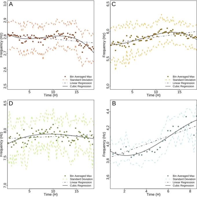
2.5 Zoom-in of frequency bands of interest observed in Figure 2.4. A close up of 2.5-3, 3.5-4.5, 5-6.5, 7-8.5 Hz frequency bands are shown in Panels A, B, C, D, respectively. Cubic and linear regressions display a drifting trend of the bin averaged maxima. . . 10
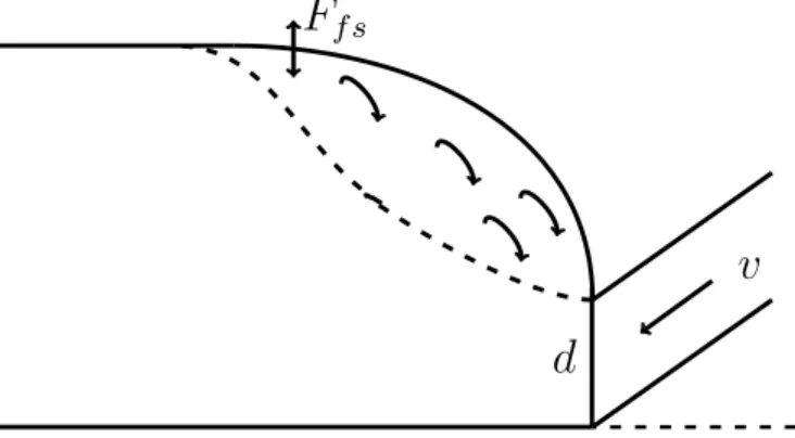
3.1 Schematic of a hydraulic jump. The Froude number (Fr) is a dimensionless parameter that quantifies the jump’s shape and activity. Thickness (d) and upstream surface velocity (V) measurements were taken for each wave shape to calculate the Fr. Ff s represents the surface oscillations of the backside of the jump. . . 14
3.3 Column 1: Measured geometrical parameters associated with each hydraulic jump: d is the height of the water column at the lowest point in the jump,
v is the velocity of the incoming fluid, Fr is the Froude number, FB refers to flash boards (O denotes open, C denotes closed, and numbered values below FB are the pressure of the flash board in PSI). Column 2: Visual description of jump parameters. Waves A, B, C and D; the person in the Wave B photo provides a sense of scale. Note that the photo of Wave A is taken from a slightly different perspective compared to the other waves. . . 16
3.4 River discharge measured at the Glenwood bridge USGS gauge station 4.8 km downstream of HWMD and pool height of HWMD. Vertical rectangles indi-cate the time intervals of seismo-acoustic observations analyzed during each Froude regime. . . 17
3.5 Network averaged Welch power spectral density (PSD) estimates of seismic and acoustic fields during each wave shape. Both data sets are filtered be-tween 0.1 and 100 Hz and are presented as dB relative to (m/s) for seismic and P a for acoustic signals. Thin vertical lines surrounding the spectra rep-resent the variance at each frequency with 95% confidence intervals. Cyan (2-5.5 Hz) and orange (9-25 Hz) rectangles represent regions of interest. . . 21
3.6 Panels A (Fr 1.03), B (Fr 1.43), C (Fr 1.77), and D (Fr 1.99) display net-work averaged cross-spectral coherence estimates of the acoustic wave field surrounding each Froude regime. The corresponding network averaged PSD is superimposed for comparison. Cross-spectral coherence results are binned into 1 Hz bins and statistics are computed; mean is shown in cyan, and the standard deviation is displayed by gray dashed lines. Waves A and B do not display elevated coherence values centered around specific frequencies, indi-cating a lack of coherent acoustic signal. Waves C and D contain distinct peaks of increased coherence. These frequency peaks are also observed in the PSD estimate. Rectangles indicate the margins of the bandpass filter used in semblance analysis. . . 23
3.8 Examples of non-cohesive (A, Figure 3.3:Wave C) and cohesive (B, Fig-ure 3.3:Wave D) standing river waves. The cohesive featFig-ure acts as a con-sistently oscillating unit on the surface of the wave, while the non-cohesive features functions as multiple surficial units operating independently of one another. Figure 3.8 is drawn with a perspective point of view. . . 30
4.1 Map of Big Falls study Area. The green is replaced with NIR to highlight turbulent river features in arial imagery with 1 m resolution. Red triangles denote Gems microphones. The x over a triangle denotes a microphone that produced corrupted data. . . 34
4.2 Discharge measured the USGS gauge in Lowman, ID. Discharge data is highly variable and displays multiple local maxima during the Big Falls study period that lasted for 2500 hours. . . 34
4.3 Bandpass filtered time series data between 3-7 Hz of each node in the Gems network. Gems experimental instrumentation displays correlation across the network suggesting that nodes are synced in time and responsiveness. This correlated network response suggest the usefulness of the Gem as a fluvial acoustic instrument. . . 35
4.4 Panel A shows network averaged Welch power spectral density (PSD) es-timates of the acoustic field surrounding Big Falls Rapid. Both data sets are filtered between 0.1 and 100 Hz and are presented as dB relative to P a. Thin vertical lines surrounding the spectra represent the variance at each frequency with 95% confidence intervals. Panel B denotes network averaged cross-spectral coherence estimates of the acoustic wave field near Big Falls. The corresponding network averaged PSD is superimposed for comparison. Cross-spectral coherence results are binned into 1 Hz bins and statistics are computed; mean is shown in black, and the standard deviation is displayed by grey dashed lines. Grey rectangles indicate the margins of the band pass filter used in semblance analysis. . . 37
A1 Verification that Meridian Compact Seismometers were calibrated during the 6/23/2017 Boise River Park experiment. We used a magnitude 5.8 earth-quake that occurred at Latitude 23.68 North, Longitude 123.36 East and was detected by the seismic array deployed at the Boise River Park (BSM2-BSM7). We compare time series data collected with the the Boise River Park array to an IRIS station MFID located at Latitude 43.41 North, Longitude -115.83 East approximately 40 km south-east of the Boise River Park. Data is band-pass filtered between 10-100 seconds. . . 44
A2 Coherent Meridian Compact Seismometers are displayed. Seismic data are from the earthquake explained in Figure caption A1. . . 45
C1 Image of Nikki’s Notch Rapid at Flood stage. Photo taken during Hurricane Joaquin 8/3/2015. . . 93
C2 Photo of the week Boise State University 5/18/2916. Photo taken during the Boise Whitewater park experiment one. Note: ADV had too much variance to capture wave velocity field. . . 94
C3 Image of Big Falls Rapid with acoustic oscillators highlighted by text. Person is in the image for scale. . . 94
C4 Image of Jake Anderson and Tim Ronan at Big Falls Rapid. True school colors are shown. . . 95
CHAPTER 1. Introduction
Rivers are known to generate infrasonic and seismic energy [Johnson et al., 2006; Burtin et al., 2008; Schmandt et al., 2013]. Discharge-dependent excitation of seismic and/or acoustic wave fields near rivers suggest that energy is transferred from fluvial hydraulic head into seismo-acoustic waves. Recent work has sought to determine and de-scribe the mechanisms that generate these energy fields around rivers [Burtin et al., 2008; Tsai et al., 2012;Schmandt et al., 2013;Gimbert et al., 2014]. The proposed mechanisms include turbulence [Burtin et al., 2008; Gimbert et al., 2014], sediment transport [Burtin et al., 2008; Hsu et al., 2011], and fluid traction between laminar flowing water and the bottom of the river [Schmandt et al., 2013]. Hysteresis observed in the seismic field above 1 Hz, led early studies to emphasize the role of sediment transport as a primary mech-anism of seismic energy generation during seasonal cycles with varied discharge [Burtin et al., 2008; Hsu et al., 2011]. More recently, investigators have begun to associate dis-tinct frequency bands within the seismic and acoustic spectra to different fluvial processes [Schmandt et al., 2013]. If existent, correlations between seismo-acoustic spectral obser-vations and river conditions could be used to remotely monitor fluvial systems through the ambient seismic and acoustic signals observed near rivers.
• Chapter 2: Linville Gorge: New Territories in Fluvial Acoustics
• Chapter 3: Harry W. Morrison Dam: Fluvial Seismo-Acoustics of Variable Hy-draulic Jumps
• Chapter 4: Big Falls: Locating Acoustic Resonators in a Flooding Target
CHAPTER 2.
Linville Gorge: New Territories in Fluvial Acoustical Studies 2.1 Introduction
To the best of my knowledge, Schmandt et al. [2013] is the only geophysical study to report ambient infrasound next to turbulent whitewater rapids. This study reported a consistent spectral peak of 6.25 Hz throughout a flood cycle of the Hance Rapid on the Colorado River. AlthoughSchmandt et al. [2013] reported hysteresis in finite seismic spectral bands, they ignored spectral variations in the near river infrasound that could be controlled by the river’s changing discharge. The Linville Gorge experiment was an attempt to corroborate Schmandt et al. [2013] infrasound result. Furthermore, the Linville Gorge experiment was designed to test the first hypothesis of my study: The ambient acoustic pressure surrounding high gradient rapids changes in amplitude and spectral content during high discharge events.
2.2 Study Site
−10−20 0 10 20 30 40 50
−10
0
10
20
Distance (m)
Distance (m)
Mi Mj Mi
N
Flow
Figure 2.1: Map of Linville Gorge Study area. Nikki’s Notch is the first rapid
down-stream of the Cathedral Gorge on the Linville River, NC. At this rapid, wa-ter is directed through a channel that is approximately 1 m wide. Directly downstream of this channel is a boulder with an approximate base width of 10 m
generate a high volume steady hydraulic jump [Te Chow, 1959] throughout the
ini-tial 11 hours (approximately) of the Linville Gorge experiment.
Discharge data downloaded from the Nebo, NC. gauge station, located approximately 13.5 km downstream of Nikki’s Notch rapid (NNR), display values between 21.1-83.3
m3/s during the 18 hour Linville Gorge study period (10/3/2015-10/4/2015) [USGS,
2016] (Figure 2.3). During this study, the peak reported discharge was approximately 5850% of the historic median for this date [USGS, 2016]. Flood conditions occurred because of rain generated by Hurricane Joaquin, a category 4 hurricane with its origin in the central Bahamas [Berg, 2015].
2.3 Data Acquisition
Three InfraBSU sensors were linearly arranged parallel to the Nikki’s Notch rapid to capture phase lags in the arrival of acoustic signals (Figure 2.1). InfraBSU sensors are flat in the band above 0.04 Hz and are MEMS-based transducers similar to sensors described in Marcillo et al. [2012]. Data was logged to an Omnirecs Datacube recording at 100 samples/second (sps). Raw waveform amplitudes were converted to physical units using conversion factors specific to the sensitivity of the InfraBSU microphones and the Datacube’s gain setting. All data were detrended.
2.4 Data Analysis Methods
frequency content of boxcar maxima to those parameters of the index signal. Discharge is compared to the variance of the acoustic amplitude so trends can be identified.
2.4.1 Power Spectral Density
Estimates of the average power-spectral density (PSD) of time series data are gen-erated by calculating the Welch averaged PSD ¯Pi(f) of instrument i [Welch, 1967] (fol-lowing Burtin et al. [2008]). Welch PSD are calculated by averaging the spectra of incrementing k boxcar windows (Bk(f)):
¯
Pi(f) =
1
k
k
X
k=1
Bk(f). (2.1)
The spectral variance is calculated at each frequency f as the averaged covariance of the spectral content of k−1 subsequent boxcar windows (Bk(f)) [Welch, 1967]:
d(j) = Covariance{Bk(f), Bk+1(f))}, (2.2)
V ar{P¯i(f)}=
1
j
k−1
X
j=1
d(j). (2.3)
The Welch PSD and the associated variance is then spatially averaged across the instrument network
A(f) = 1
M
M
X
i=1
¯
Pi(f), (2.4)
where M is the total number of instruments. Temporally and spatially averaged PSDs provide a robust estimate of the seismic and acoustic frequency content contemporaneous with each wave shape. Spectra are presented as decibels relative to the unit of instrument sensitivity.
variance by separating the acoustic time series into 2048 boxcar windows of 100 s that were incremented by 5 s (Appendix 5).
2.4.2 Temporal Acoustic Variance
I captured temporal variance of the acoustic wave field surrounding the NNR and relate this variance to the discharge of a Linville Gorge flood cycle. First, I separated the time series data into incrementing boxcar windows (Bk,i). Spectral content of each boxcar (Bk,i(f)) is found using the Fast Fourier transform code in the R programming language [R Core Team, 2013]. The amplitude and position of local maxima in each window’s spectral domain are estimated and spatially averaged across the microphone array.
A(f) = 1
3
3
X
i=1
M ax(Bk,i(f)), (2.5)
2.5 Results
The Linville Gorge experiment was a preliminary study displaying that high gradient rapids produce acoustic signatures with spectral peaks in finite frequency bands. This study was purposefully conducted during Hurricane Joaquin, a period of high discharge variance, and acoustic signals were compared to discharge. Study results show a corre-lation between discharge and the amplitude of the acoustic pressure field. Furthermore, the frequency contents of acoustic spectral maxima display temporal variance from the index spectral signature suggesting that the river stage partially controls the acoustic signal.
2.5.1 Acoustic Power Spectral Density
0 5 10 15 20 25
−20
−15
−10
−5
0
P
o
w
er (dB)
Frequency (Hz)
PSD Variance 2.5−3 Hz Band
3.5−4.5 Hz Band 5−6.5 Hz Band 7−8.5 Hz Band
Figure 2.2: Spatially and temporally averaged power spectral density of the acoustic wave field surrounding Nicki’s Notch rapid during the Linville Gorge study from 10/3/2015-10/4/2015. PSD estimates display peak frequency bands of 2.5-3, 3.5-4.5, 5-6.5, and 7-8.5 Hz that are denoted by vertical colored rectangles. Nicki’s Notch Rapid on the
Linville Gorge, NC. generates in-frasound with spatially and tem-porally averaged peak frequen-cies of approximately 2.8,4.0, 5.8, and 7.8 Hz under spe-cific flow conditions (Figure 2.2). The 2.8 Hz frequency peak dis-plays the highest amplitude and is narrow band compared to
is generated from nearly 18 hours of data. Spectral bands of higher frequencies are more similar to the ambient background noise. The frequency peaks centered around 5.8 and 7.8 Hz are relatively broadband and low amplitude compared to the 2.8 Hz peak.
2.5.2 Acoustic Amplitude
5 10 15
3.0
3.5
4.0
4.5
5.0
5.5
6.0
Pressure (P
a)
Time (H)
300
400
500
600
700
800
900
Discharge (m^3/s)
Discharge 2.5−3 Hz Band 3.5−4.5 Hz Band
5−6.5 Hz Band 7−8.5 Hz Band Bin Averaged
Figure 2.3: Bin averaged acoustic amplitudes across all frequency bands of interest and the time series grid. Discharge (m3/s) sampled at 15 m is presented as a solid grey line
so river conditions and the acoustic wave field can be compared.