Rationalizing spatial exploration patterns of wild
animals and humans through a temporal
discounting framework
Vijay Mohan K. Namboodiria,b,1, Joshua M. Levyc,1, Stefan Mihalasd, David W. Simse,f,g, and Marshall G. Hussain Shulerc,2
aDepartment of Psychiatry, University of North Carolina, Chapel Hill, NC 27599;bNeuroscience Center, University of North Carolina, Chapel Hill, NC 27599; cDepartment of Neuroscience, Johns Hopkins University, Baltimore, MD 21205;dAllen Institute for Brain Science, Seattle, WA 98109;eMarine Biological
Association of the United Kingdom, The Laboratory, Plymouth PL1 2PB, United Kingdom;fOcean and Earth Science, National Oceanography Centre
Southampton, University of Southampton, Southampton SO14 3ZH, United Kingdom; andgCentre for Biological Sciences, University of Southampton,
Southampton SO17 1BJ, United Kingdom
Edited by H. Eugene Stanley, Boston University, Boston, MA, and approved May 26, 2016 (received for review February 1, 2016)
Understanding the exploration patterns of foragers in the wild provides fundamental insight into animal behavior. Recent exper-imental evidence has demonstrated that path lengths (distances between consecutive turns) taken by foragers are well fitted by a power law distribution. Numerous theoretical contributions have posited that“Lévy random walks”—which can produce power law path length distributions—are optimal for memoryless agents search-ing a sparse reward landscape. It is unclear, however, whether such a strategy is efficient for cognitively complex agents, from wild animals to humans. Here, we developed a model to explain the emergence of apparent power law path length distributions in animals that can learn about their environments. In our model, the agent’s goal during search is to build an internal model of the distribution of rewards in space that takes into account the cost of time to reach distant loca-tions (i.e., temporally discounting rewards). For an agent with such a goal, we find that an optimal model of exploration in fact produces hyperbolic path lengths, which are well approximated by power laws. We then provide support for our model by showing that hu-mans in a laboratory spatial exploration task search space system-atically and modify their search patterns under a cost of time. In addition, we find that path length distributions in a large dataset obtained from free-ranging marine vertebrates are well described by our hyperbolic model. Thus, we provide a general theoretical framework for understanding spatial exploration patterns of cogni-tively complex foragers.
Lévy walks
|
temporal discounting|
optimal search|
decision making|
foraging theoryL
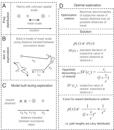
évy walks are a special kind of random walk whose path lengths form a power law distribution at their asymptotic limit (x):pðxÞ∝x−μ; 1<μ<3; x>xmin(1–4). Numerous recent papers have demonstrated that foraging animals in the wild or under controlled conditions show path lengths consistent with power laws (5–11), which are proposed to arise from an underlying Lévy walk process. Theoretical models have demonstrated that such a process can be optimal for memoryless agents searching for randomly distributed rewards across space under certain condi-tions (1, 2, 12). Together, these findings have led to the Lévy flight foraging hypothesis, which states that such search patterns have arisen due to their evolutionary advantage (2, 3). However, be-cause many animals, including humans, are cognitively complex and can learn from their environments, it is important to address whether such heavy-tailed path lengths are optimal even for cog-nitively complex agents (Fig. S1). The question of how memory influences foraging patterns has been approached in some con-texts (13–16) but has not yet been sufficiently addressed (17–20). Because power law path lengths have been observed in sparse and dynamic environments (e.g., open ocean), in which foragers rarely revisited previously rewarded locations (8, 10, 21, 22), it isreasonable to assume, as foundational models have, that there is little advantage to learning about the reward distributions at any given spatial location. Hence, under this assumption, prior studies constrained the class of models studied to random searches in the absence of learning. However, despite the fact that remembering spatial locations in environments such as open oceans may not be advantageous, it is widely believed that many ecological parameters, including prey distributions, show high degrees of spatial autocorre-lation (23, 24). Moreover, it has been found that these distributions can exist as hierarchies, wherein large, global spatial structures com-prise smaller, more local structures, and that predators potentially learn these mean scales in the spatial distribution of prey (23, 24). Therefore, given the existence of patterns in the distribution of prey in relative space, it may be advantageous for predators to build repre-sentations, or models, of these patterns as opposed to performing purely random searches (Fig. 1AandB). In this paper, we show that to optimally learn the reward distribution across relative spatial scales in the service of future reward rate maximization, foragers would produce approximate power law path lengths, resembling Lévy walks. How might foragers build a model of the relative spacing be-tween food items? Consider the foraging behavior of albatrosses,
Significance
Understanding the movement patterns of wild animals is a fundamental question in ecology with implications for wildlife conservation. It has recently been hypothesized that random search patterns known as Lévy walks are optimal and underlie the observed power law movement patterns of wild foragers. However, as Lévy walk models assume that foragers do not learn from experience, they may not apply generally to cognitive animals. Here, we present a decision-theoretic framework wherein animals attempting to optimally learn from their environments will show near power law-distributed path lengths due to tem-poral discounting. We then provide experimental support for this framework in human exploration in a controlled laboratory set-ting and in animals foraging in the wild.
Author contributions: V.M.K.N., J.M.L., S.M., and M.G.H.S. designed research; V.M.K.N. and J.M.L. performed research; V.M.K.N. and J.M.L. analyzed data; V.M.K.N., J.M.L., D.W.S., and M.G.H.S. wrote the paper; S.M. contributed to mathematical aspects of theory; and D.W.S. contributed data.
The authors declare no conflict of interest.
This article is a PNAS Direct Submission.
Freely available online through the PNAS open access option.
See Commentary on page 8571.
1V.M.K.N. and J.M.L. contributed equally to this work.
2To whom correspondence should be addressed. Email: [email protected].
This article contains supporting information online atwww.pnas.org/lookup/suppl/doi:10. 1073/pnas.1601664113/-/DCSupplemental.
ECOLO
GY
SEE
COM
for instance. A straightforward solution is to build a model of rewards obtained as a function of distance flown on each step (Fig. 1C). Because the speed of movement during searching is often nearly constant for many foragers (e.g., refs. 8 and 16), this model can also be built with respect to the time flown on each step. The question faced by the forager then becomes how to sample different step lengths to maximize the ability to detect differences in reward distributions associated with each step length. However, foragers do not treat the same reward available at different delays equally: The later the receipt of a reward is, the lower its subjective value (26, 27). In other words, the subjective value of a reward expected after a long flight is smaller than that of the same reward obtained immediately. Many behavioral experiments have shown that the cost of time associated with a delayed reward takes a specific functional form: that of a hyperbolic (for μ = 1) or hyperbolic-like (forμ≠1) function (26–33), shown as
SVðr,tÞ=rDðr,tÞ= r
ð1+t=cÞμ, [1] where SV(r, t) and D(r, t) represent the subjective value and discounting function, respectively, of a reward of magnitude r
delayed by a timet.candμrepresent parameters that measure the rate at which the value of a delayed reward is discounted. In light of such a cost of time, exploration of a given flight time should be done under consideration of its utility for future ex-ploitation. Thus, the foragers must explore to maximize their
ability to discriminate subjective value (not reward) distributions associated with different step lengths.
Here, we show that to maximize the ability to discriminate the subjective value distributions associated with different step lengths, the forager has to sample each step length in proportion to the uncertainty in subjective value associated with that step length (SI Results,2.1) Optimal Exploration of Reward Distributions Across Relative Spaceand Fig. 1D). This strategy makes intuitive sense because the higher the uncertainty associated with an option, the more it must be sampled to learn its properties. Such a strategy of exploring in proportion to uncertainty has previously been as-sumed to be an exploration heuristic (34). However, we show that it is in fact optimal for maximizing discriminability (SI Results,2.1) Optimal Exploration of Reward Distributions Across Relative Space). For a forager that initiates exploration under a uniform prior (i.e., no a priori assumption regarding the distribution of rewards), sampling in proportion to uncertainty in subjective value equates to sampling in proportion to the discounting function associated with a flight time. As previously mentioned, the discounting function over flight time is hyperbolic. Therefore, for constant speed, the discounting function for a path length is also hyperbolic. Thus, we predict that the path length distribution of a forager attempting to explore the reward distribution across relative space will be
pðxÞ∝ 1
ð1+x=cÞμ; or rearranging by a constant, pðxÞ∝ 1
ðc+xÞμ. [2]
This is similar in appearance to a power law, but differs due to the presence of an additive constantc. Consequently, whereas it decays asymptotically as a power law, it predicts a constant probability at low values. Further, note that any distribution that is consistent with a strict power law [e.g., prior observations of foraging patterns (8–10)] will necessarily be consistent with the above distribution because the power law distribution is a special case of Eq. 2in which c= 0. Because foragers might limit the range of their exploration to a bounded interval of step lengths (e.g., due to behavioral/environmen-tal constraints), the above probability distribution would be expected to hold only in a truncated domain (betweenxminandxmax) under exploration. Further, in reward dense environments, we propose that observed path lengths would reflect not just the intended path lengths shown in Eq.2, but also the truncation due to prey encounter, thus resulting in exponential path lengths [as has previously been shown (7)] (SI Results,2.4) Truncation Due to Prey EncounterandFig. S2). The model described above makes several predictions about search behavior of a cognitively complex agent that we could test with humans in a controlled laboratory setting. Specifically, we sought to determine (i) whether humans search space in a random search pattern as expected from the Lévy walk model or in a sys-tematic and deterministic way and (ii) whether spatial search pat-terns are sensitive to the cost of time incurred in traversing the space. To test this, we designed a spatial exploration task for hu-mans with and without the cost of time (Methods, Fig. 2A, andSI Discussion,1.1) Human Exploratory Task). In phase 1 (with a time cost) of this task, subjects could stop an image of a flying albatross to reveal a fish at a given spatial location. The goal of the subjects was to build a model of the distribution of fish as the knowledge acquired during this exploration phase could then be used on one exploitation trial to collect the largest fish possible. Crucially, flying longer distances across the screen took proportionally more time (the longest distance corresponded to waiting 10 s). Unknown to the subjects was that the distribution of fish sizes at any given lo-cation was uniform between fixed bounds. To test path lengths in the absence of a time cost, we removed the distance–time re-lationship in phase 2 and allowed the subjects to explore by merely clicking a given location with a computer mouse. In other words, they no longer had to wait for the albatross to fly to that location.
A
B
C
D
We found that in both phases, the pattern of search was nonrandom. Subjects systematically explored the space by, for instance, undertaking longer and longer path lengths or un-dertaking shorter and shorter path lengths from the end of the screen (see Fig. 2Bfor two example subjects andFig. S3for all subjects). Statistically, the probability of finding bouts of posi-tive path length differences or negaposi-tive path length differences between consecutive paths was higher than chance in every subject for phase 2 (P<0.05, runs test with Benjamini–Hochberg correction for multiple comparisons,n=12). For phase 1, the nonrandomness in the search was statistically significant in 10 of 12 subjects (P< 0.05, runs test with Benjamini–Hochberg correction for multiple comparisons). Thus, human spatial search in this random environment is not random. This conclusion is also bolstered by prior studies demonstrating that numerous animals remember spatial locations to produce nonrandom spatial search patterns in the wild (20, 35–41). We also found that the distri-bution of path lengths in phase 1 was significantly different from that in phase 2 (Fig. 2C;P<0.001, two-tailed two-sample Kolmogorov–Smirnov test) due to the cost of time, as predicted by our temporal discounting model. Thus, human data support two key predictions of our model, i.e., that spatial search by cognitively complex agents is systematic and nonrandom and that temporal discounting plays a fundamental role in the shaping of such a search. These datasets are relatively small, however—as it is dif-ficult to encourage human subjects to explore for long periods in a laboratory setting—and, therefore, are insufficient for model comparisons (although our model is consistent with the data). Therefore, to perform model comparisons, where considerable amounts of data are required (Fig. 3A), we turned to foraging data in the wild where, in some instances, thousands of path lengths have been recorded from individual animals.
Given the preponderance of evidence that foraging path lengths are well fitted by the power law distribution (5–9), the immediate question to be addressed is whether the hyperbolic distribution of path lengths expected from Eq.2can be well described by a power law. Because the above distribution (and a power law) is defined in a bounded domain, we tested against a truncated power law (seeMethods for details). We found that for random numbers generated using Eq. 2, Akaike information criterion weights (wAIC) overwhelmingly support a truncated power law compared with a truncated exponential (wAICtp = 1.000 and wAICexp = 0.000) for all parameters tested (Fig. 3AandFig. S4).
At this point, we wondered whether previously analyzed for-aging data (8) may be well explained by our model. For this analysis, we compared a hyperbolic model to a power law model, as the power law distribution was found to provide a good fit to the data (8) and is generally compared against the exponential distribution to assert the presence of Lévy walks (5–7, 9–12). To
be clear, we compared against the power law distribution, not the family of distributions that have power law distributions at their asymptotic limits—to which a hyperbolic and a power law model both belong. One important point to note here is that whereas a strict power law distribution is a special case of the hyperbolic distribution, it is not necessarily true that in a direct comparison between the two models the data will be better fitted by a hy-perbolic distribution. If the path length distributions decay as steeply or more steeply than a power law, the best fit hyperbolic model will reduce to the best fit power law and, hence, model selection (bywAIC) would favor the model with fewer parame-ters (i.e., the pure power law model).
Because differentiating between two highly similar distribu-tions requires considerable statistical power, we limited our test to eight individual marine animals, comprising four blue sharks
Prionace glauca(PG) and four basking sharksCetorhinus maximus
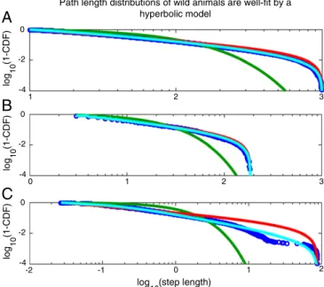
(CM), for which a substantial number of path lengths (>10,000) were recorded. The results for two individuals, blue sharks PG2 and PG4, are shown in Fig. 3BandC, respectively. In both cases, the hyperbolic fit (cyan) provides an excellent fit to the data. Notably, the truncated power law fit is visually compelling for PG2 (Fig. 3B) but not for PG4 (Fig. 3C). Indeed, individual PG2 represents a typical case where the fits are not easily distin-guishable visually (as in the simulation in Fig. 3A), but where the
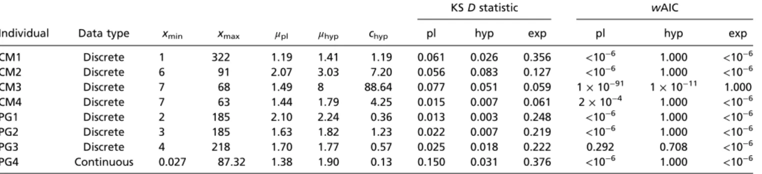
wAIC overwhelmingly favors a hyperbolic model. Examining all individuals, we found that the hyperbolic model provided a su-perior explanation of the data compared with power law and ex-ponential models in all but one individual (Table 1). In this individual (CM3), the exponential model provided the best fit, potentially due to prey encounter-related truncation (7). In all other cases, the hyperbolic model was overwhelmingly favored Task schematic
Travel to x (time ∝ x)
Phase 1
Fish
Teleport to x (time = 0) Phase 2
Fish
distance
trial number 40
0 0 104
distance
CDF
104 0
1
0
A
B
C
Fig. 2. Human spatial exploration task with and without temporal costs. (A) Schematic of the computer task (MethodsandSI Methods). In phase 1, an albatross flies across the screen from a nest at a constant speed. In phase 2, subjects can make the albatross teleport (i.e., flight time is negligible). (B) Data from example subjects showing systematic search behavior across space. (C) Raw cumulative distribution function (CDF) of the population data across subjects for phase 1 and phase 2, showing sensitivity of exploration to the cost of time.
log
10
(1-CDF)
0
-2
-4
log
10
(1-CDF)
0
-2
-4
log
10
(1-CDF)
0
-2
-4
1 2 3
0 1 2 3
-2 -1 0 1 2
log (step length)
Path length distributions of wild animals are well-fit by a hyperbolic model
A
B
C
Fig. 3. Previously collected data from wild animals are better fitted by a hyperbolic model than by a power law model. (A) Random data generated from a hyperbolic distribution (blue circles) can be well approximated by a power law distribution (red), but not by an exponential distribution (green): 25,000 random numbers were generated from a hyperbolic distribution (Eq.2) (Methods) with truncation set to be between 10 and 1,000 (seeFig. S4for more parameters). The best fit truncated power law describes the data significantly better than the best fit exponential (wAICtp=1.000 andwAICexp=0.000).
(B) Previously collected data (blue circles) that are well fitted by a hyperbolic model (cyan) and a power law model (red), but not by an exponential model (green) (seeFig. S5for fits across many subjects). (C) Data from a subject in which the hyperbolic model is considerably preferred to any alternative model.
ECOLO
GY
SEE
COM
(wAIC=1.000), except in PG3 where support was not as clear-cut (wAIC= 0.708). Hence, our theoretical model provides a superior fit to previously collected foraging data.
In our model for foraging animals in the wild, we previously assumed perfect ability to estimate the time flown in a given step. Because we know that the error in estimating longer intervals is larger than that in estimating shorter ones (42), we derived the optimal exploration model for the biologically realistic case in which time perception is subjective and noisy (Fig. 4). In this model, the sampling per bin of path length (or equivalently, real time) for maximizing discriminability of rewards associated with that path length is determined by the degree of nonlinearity in time percep-tion as different bins in subjective time are scaled differently, depending on the nonlinearity (Fig. 4C). Theoretically, it has been proposed previously that the degree of nonlinearity in time per-ception is directly related to the discounting function in subjective time (43) (Fig. 4D, Left). Consequently, we show—based on our prior theory of temporal perception and decision making (43–46)— that the optimal path length distribution would be
pðxÞ∝ 1
ðvTime+xÞ3
. [3]
Here,vis the speed of the animal. The termTimeis the interval over which the past reward rate experienced by an animal is estimated to make appropriate intertemporal decisions that max-imize reward rates (43–45). Importantly, this term governs the nonlinearity of time perception and the steepness of temporal discounting (43–46) (SI Results, 2.1.5) Exploration under noisy temporal estimation). Thus, the power law that best approximates the above distribution would have an exponent determined by the nonlinearity of time perception (Fig. 4D;SI Results, 2.1.5) Exploration under noisy temporal estimation; andFig. S6).
It is important to note that the derivations mentioned above necessarily simplify the foraging problem faced by animals in the wild. For instance, one factor that we did not yet take into ac-count is that animals might acac-count for other sources of risk such as that resulting from competition in their exploratory model. In such a case, we show inSI Results, 2.1.6) Modeling risk due to competition that the probability distribution of path length du-rations can be calculated as
pðtÞ∝ 1
ðTime+tÞ3ð1+kαrαtÞ1=α
, [4]
wherekandαrepresent the magnitude of competition such that an increase in their values represents more competition and
hence, shorter path lengths.rin Eq.4can be thought of as the mean reward expected in an environment; the larger the mean reward expected is, the larger the competition and the shorter the path lengths. The asymptotic limit of Eq.4, for positive α, will have a power law exponent greater than 3 and hence will be outside the Lévy range of exponents. However, in cases where the asymptotic limit cannot be reached, as is often the case in biology where path lengths are often truncated either by the physical world or potentially by some internal limit set by the forager, a best fit truncated power law will appear to have a lower exponent than the real generative process, with the apparent exponent lying between 0 and 3+1/α.
An even more complete model of animal movements would involve additional factors, some of which are mentioned inSI Discussion,1.2) Potential Predicted Deviations from the Simplified
Table 1. Data from model fits to step length distributions of eight sharks
KSDstatistic wAIC
Individual Data type xmin xmax μpl μhyp chyp pl hyp exp pl hyp exp
CM1 Discrete 1 322 1.19 1.41 1.19 0.061 0.026 0.356 <10−6 1.000 <10−6 CM2 Discrete 6 91 2.07 3.03 7.20 0.056 0.083 0.127 <10−6 1.000 <10−6 CM3 Discrete 7 68 1.49 8 88.64 0.077 0.051 0.059 1×10−91 1×10⁻¹¹ 1.000 CM4 Discrete 7 63 1.44 1.79 4.25 0.015 0.007 0.061 2×10⁻⁴ 1.000 <10−6 PG1 Discrete 2 185 2.10 2.24 0.36 0.013 0.003 0.248 <10−6 1.000 <10−6 PG2 Discrete 3 185 1.63 1.82 1.23 0.022 0.007 0.219 <10−6 1.000 <10−6 PG3 Discrete 4 218 1.70 1.77 0.57 0.025 0.018 0.222 0.292 0.708 <10−6 PG4 Continuous 0.027 87.32 1.38 1.90 0.13 0.150 0.031 0.376 <10−6 1.000 <10−6
The first seven animals had quantized data that could be considered as resulting from a discrete probability distribution. For these animals, we divided the data by their common factor to get the discrete data (e.g., the first animal had unique observations 1, 2, 3,. . ., 322).xminandxmaxrepresent the best fit truncation across all
three distributions (Methods). The maximum step length and percentile ofxmaxfor each animal were 322 (100th percentile), 91 (100th percentile), 78 (92nd percentile),
80 (80th percentile), 965 (84th percentile), 910 (80th percentile), 958 (80th percentile), and 87 (100th percentile), respectively. The best fit parameters for the power law and hyperbolic distributions are shown. The goodness-of-fit was quantified by the KSDstatistic and the relative quality of fit was quantified bywAIC.
A
B
C
D
Fig. 4. Optimal exploration when temporal representations are noisy. (A) Optimal algorithm for exploration. (B) If temporal resolution is constant at every interval, subjective representation of time can be represented as a linear function of real time, with constant noise. However, it is known that errors in timing increase with the interval being timed (42). In this case, subjective repre-sentation of time can be represented as a nonlinear function with the nonlinearity controlled by the parameterTime(43–45). (C) When subjective representation
of time is nonlinear (concave), equal bins in subjective time correspond to bins of increasing width in real time. (D) A theory of reward rate maximization (43–45) predicts linear sampling for optimal exploration in subjective time, with the slope determined byTime. In real time, this sampling becomes
hy-perbolic (Eq.3) with its decay controlled byTime(SI Results,2.1.5) Exploration
Model Presented Here. Nevertheless, the simplified model pre-sented here demonstrates that the path lengths of foragers with spatial memory who build a map of their environment for future exploitation can be heavy tailed and nearly power law distributed. To conclude, we argue that if foragers seek to learn about their reward landscape, an optimal model of exploration would require sampling in proportion to the uncertainty in subjective value associated with a reward obtained after a given path length. Because it is often observed that the subjective value of rewards obtained after a delay is discounted hyperbolically with respect to the delay, we showed that the resultant path lengths would be hyperbolically distributed. In support of our model, we found that humans engaged in a laboratory exploration task searched space systematically and account for the cost of time in traversing space. Next, we showed that data generated from a hyperbolic distribution are better fitted by a power law distribution than by an exponential distribution and that previously collected data from foraging animals in the wild can be better explained by a hyperbolic model than by a power law model. Additionally, we extended our model to show that for foragers in the wild with noisy temporal perception, the exponent of the best fit power law is governed by the nonlinearity of time perception and the amount of competition faced from other foragers. Thus, we contribute to the ongoing discussion regarding the mechanistic origins of power law path lengths in foragers (47–58) by arguing that search patterns are unlikely to be purely random when cognitive modeling is advantageous and that approximate power law path lengths emerge due to the temporal discounting of far-ther away rewards. A deeper understanding of the neurobiological basis of spatial search (59–63) may further enrich this model and provide greater insight into the movements of wild ani-mals and humans.
Methods
Description of Experiment.
Subjects.The 12 subjects that participated in this experiment were healthy individuals aged 22–35 y recruited from Johns Hopkins University. All pro-cedures were approved by the Institutional Review Board at Johns Hopkins School of Medicine under application identification NA_00075036. All sub-jects gave oral consent before the start of the experiment.
Exploration task.We developed an exploration task for human subjects. Our task was divided into two phases. At the start of each trial in phase 1, an image of an albatross would begin flying (i.e., moving) from its“nest”left to right across the“sky”(i.e., light blue patch of screen). Subjects were instructed to stop the albatross at any point by clicking a mouse. When the albatross was stopped, it would instantaneously dive into the“water”(i.e., dark blue patch of screen) and an image of a fish would be revealed. Un-known to the subject, the size of the fish was drawn from a uniform dis-tribution with five discrete outcomes. After the fish was displayed for 1 s, the albatross returned to its nest and immediately began to fly in the next trial. In phase 1, it would take the albatross 10 s to fly the entire length of the screen. The speed of the albatross was constant and was 109 pixels per second. If the subject waited for the albatross to traverse the entire screen, the albatross automatically dove into the water and a fish was revealed. Before the start of phase 1, subjects were informed that they would have exactly 3 min to explore the region and“discover where the biggest fish swim.”They were also informed that at the end of the phase, they would be given just one chance to catch the largest fish they could and that their payout would be“determined exclusively by the size of the fish on this one trial”and not by the fish caught during exploration. In this way, the subjects were incentivized to explore the region.
Following phase 1, phase 2 began. In phase 2, the subjects were instructed that the albatross was flying over a different region of the ocean and, thus, they had to explore again to know where the biggest fish swim. The albatross remained in its nest until the subject clicked on a region of space (indicated by a gray region that ran the length of the screen) to which it instantaneously teleported. Therefore, there was no time cost in exploring farther regions of space, as there was in phase 1. The instructions for phase 2 were similar to those for phase 1 except that subjects were informed that they had 1 min to explore the region. This limit was imposed so that subjects would complete a similar number of trials in phase 1 and phase 2 (because trials in phase 2
are shorter as the albatross teleports rather than flies). Aesthetic changes (background color, fish image, and fish size) were made between phases to encourage exploration by underscoring the instruction that the environ-ments in phase 1 and 2 were distinct.
Procedure.Subjects were placed in a quiet room in front of a 13-inch MacBook Pro. On-screen instructions were read aloud by the experimenter to ensure that the subject understood them. At the end of the experiment, subjects answered a questionnaire administered by the experimenter and were monetarily compensated for their participation.
Display.The experiment was controlled by custom-made code written in Java (JDK 6.0_65). The display was 1,220 pixels wide and 730 pixels high. The area of the fish image (i.e., the size of the fish) was a random integer value between 1 and 5 scaled by a constant factor.Movie S1shows a sample of the experiment.
Animal Foraging Data.Blue (n=4) and basking sharks (n=4) were each fitted with a pressure-sensitive data logger that recorded an individual time series of depth measurements as the fish swam through the water column, as described previously (8). Raw depth measurements from loggers were con-verted into move step lengths by calculating the vertical movement step size between successive vertical changes in direction (from down to up and vice versa), as described previously (8).
Procedure to Fit Data.The general approach used here to test the
appro-priateness of different models is to (i) estimate the respective parameters using maximum-likelihood estimation (MLE) for the same set of possible truncations across all models, (ii) set the best truncation to that resulting in the lowest Kolmogorov–Smirnov (KS)Dstatistic across all models and all truncations, and (iii) quantify relative likelihoods of models, using the AIC.
The truncated hyperbolic-like distribution, shown in Eq.2, needed to be statistically characterized. We do so inSI Results,2.2) Statistical Charac-terization of the Hyperbolic Distribution in Eq. S1. The truncated power law distribution is a particular example of a truncated hyperbolic distri-bution forc=0. To test whether data generated from this distribution can be mistaken for a power law distribution (Fig. 3A), we generated data using the following random number generator (derived inSI Results,2.2) Statistical Characterization of the Hyperbolic Distribution in Eq. S1),
t=hðtmin+cÞ1−μ+ n
ðtmax+cÞ1−μ−ðtmin+cÞ1−μ o
ui1=ð1−μÞ−c, wheretis the random variate following the truncated hyperbolic-like dis-tribution,tminandtmaxare the minimum and maximum truncation limits,c
andμare the parameters of the distribution, anduis a uniform random variate. For the purpose of Fig. 2,tminwas set at 10 andtmaxat 1,000. More
parameters are shown inFig. S4. The procedure for fitting and testing of power law, hyperbolic, and exponential models is explained below.
Prior data were tested against three models: (i) exponential, (ii) truncated power law, and (iii) truncated hyperbolic. The same truncation parameters were fitted across all models. To this end, we fitted each model at different sets of truncation and then found the truncation that resulted in the lowest KSDstatistic across all models. Thus, truncation limits are not free-fitting parameters for each distribution that add cost to the AIC. The benefit of using this approach is that the exact same data are used for comparison across all of the models, thus avoiding different domains of the probability distribution functions for the different distributions tested. The procedure for MLE is derived and explained in detail inSI Methods,3.1) Model Fits.
To calculate relative likelihood of the different models (i.e., assessing which model minimizes the estimated Kullback–Liebler divergence between data and the model), the AIC was calculated for every model as shown be-low (explained inSI Methods,3.2) Model Comparisons):
AICtp=2−2 logLtp+
4 n−2
AIChyp=4−2 log
Lhyp
+n12−3
AICexp=2−2 log
Lexp
+n4−2.
Lis the likelihood of the data given each model. We used the small-sample correction for the AIC.
ACKNOWLEDGMENTS.We thank Prof. David Foster and Prof. Ernst Niebur for comments and discussion. This work was funded by a National Institute of Mental Health Grant R01MH093665.
ECOLO
GY
SEE
COM
and mechanisms.Ecology90(4):877–887.
2. Viswanathan GM, Raposo EP, da Luz MGE (2008) Lévy flights and superdiffusion in the context of biological encounters and random searches.Phys Life Rev5(3):133–150. 3. Viswanathan GM, da Luz MGE, Raposo EP, Stanley HE (2011)The Physics of Foraging
(Cambridge Univ Press, Cambridge, UK).
4. Mendez V, Campos D, Batumeus F (2014)Stochastic Foundations in Movement Ecology: Anomalous Diffusion, Front Propogation and Random Searches(Springer, Berlin).
5. Sims DW, et al. (2014) Hierarchical random walks in trace fossils and the origin of optimal search behavior.Proc Natl Acad Sci USA111(30):11073–11078.
6. de Jager M, Weissing FJ, Herman PMJ, Nolet BA, van de Koppel J (2011) Lévy walks evolve through interaction between movement and environmental complexity.
Science332(6037):1551–1553.
7. De Jager M, et al. (2014) How superdiffusion gets arrested: Ecological encounters explain shift from Lévy to Brownian movement.Proc Biol Sci281:20132605. 8. Humphries NE, et al. (2010) Environmental context explains Lévy and Brownian
movement patterns of marine predators.Nature465(7301):1066–1069.
9. Sims DW, et al. (2008) Scaling laws of marine predator search behaviour.Nature
451(7182):1098–1102.
10. Humphries NE, Weimerskirch H, Queiroz N, Southall EJ, Sims DW (2012) Foraging success of biological Lévy flights recorded in situ.Proc Natl Acad Sci USA109(19): 7169–7174.
11. Raichlen DA, et al. (2014) Evidence of Levy walk foraging patterns in human hunter-gatherers.Proc Natl Acad Sci USA111(2):728–733.
12. Viswanathan GM, et al. (1999) Optimizing the success of random searches.Nature
401(6756):911–914.
13. Ferreira AS, Raposo EP, Viswanathan GM, Da Luz MGE (2012) The influence of the environment on Levy random search efficiency: Fractality and memory effects.Phys A Stat Mech Appl391(11):3234–3246.
14. Van Moorter B, et al. (2009) Memory keeps you at home: A mechanistic model for home range emergence.Oikos118(5):641–652.
15. Tabone M, Ermentrout B, Doiron B (2010) Balancing organization and flexibility in foraging dynamics.J Theor Biol266(3):391–400.
16. Boyer D, Walsh PD (2010) Modelling the mobility of living organisms in heteroge-neous landscapes: Does memory improve foraging success?Philos Trans A Math Phys Eng Sci368(1933):5645–5659.
17. James A, Plank MJ, Edwards AM (2011) Assessing Lévy walks as models of animal foraging.J R Soc Interface8(62):1233–1247.
18. Gautestad AO, Mysterud A (2013) The Lévy flight foraging hypothesis: Forgetting about memory may lead to false verification of Brownian motion.Mov Ecol1(1):9. 19. Gautestad AO (2011) Memory matters: Influence from a cognitive map on animal
space use.J Theor Biol287(0):26–36.
20. Fagan WF, et al. (2013) Spatial memory and animal movement.Ecol Lett16(10): 1316–1329.
21. Weimerskirch H, Pinaud D, Pawlowski F, Bost C-A (2007) Does prey capture induce area-restricted search? A fine-scale study using GPS in a marine predator, the wan-dering albatross.Am Nat170(5):734–743.
22. Weimerskirch H, Gault A, Cherel Y (2005) Prey distribution and patchiness: Factors in foraging success and efficiency of wandering albatrosses.Ecology86(10):2611–2622. 23. Fauchald P, Erikstad KE, Skarsfjord H (2000) Scale-dependent predator–prey interactions:
The hierarchical spatial distribution of seabirds and prey.Ecology81(3):773–783. 24. Fauchald P, Erikstad KE (2002) Scale-dependent predator-prey interactions: The
ag-gregative response of seabirds to prey under variable prey abundance and patchiness.
Mar Ecol Prog Ser231:279–291.
25. Sims DW, Quayle VA (1998) Selective foraging behaviour of basking sharks on zoo-plankton in a small-scale front.Nature393(June):460–464.
26. Green L, Myerson J (2004) A discounting framework for choice with delayed and probabilistic rewards.Psychol Bull130(5):769–792.
27. Stephens DW, Krebs JR (1986)Foraging Theory(Princeton Univ Press, Princeton, NJ). 28. Kirby KN, Marakovic NN (1995) Modeling myopic decisions: Evidence for hyperbolic delay-discounting within subjects and amounts.Organ Behav Hum Decis Process
64(1):22–30.
29. Green L, Myerson J (1996) Exponential versus hyperbolic discounting of delayed outcomes: Risk and waiting time.Am Zool36(4):496–505.
30. Vuchinich RE, Simpson CA (1998) Hyperbolic temporal discounting in social drinkers and problem drinkers.Exp Clin Psychopharmacol6(3):292–305.
31. Johnson MW, Bickel WK (2002) Within-subject comparison of real and hypothetical money rewards in delay discounting.J Exp Anal Behav77(2):129–146.
32. Murphy JG, Vuchinich RE, Simpson CA (2001) Delayed reward and cost discounting.
Psychol Rec51:571–588.
33. Simpson CA, Vuchinich RE (2000) Reliability of a measure of temporal discounting.
Psychol Rec50:3–16.
34. Badre D, Doll BB, Long NM, Frank MJ (2012) Rostrolateral prefrontal cortex and in-dividual differences in uncertainty-driven exploration.Neuron73(3):595–607. 35. Muller M, Wehner R (1994) The hidden spiral: Systematic search and path integration
in desert ants, Cataglyphis fortis.J Comp Physiol A Neuroethol Sens Neural Behav Physiol175:525–530.
36. Cramer AE, Gallistel CR (1997) Vervet monkeys as travelling salesmen. Nature
387(6632):464.
37. Janson CH (1998) Experimental evidence for spatial memory in foraging wild capu-chin monkeys, Cebus apella.Anim Behav55(5):1229–1243.
38. Valero A, Byrne RW (2007) Spider monkey ranging patterns in Mexican subtropical forest: Do travel routes reflect planning?Anim Cogn10(3):305–315.
39. Asensio N, Brockelman WY, Malaivijitnond S, Reichard UH (2011) Gibbon travel paths are goal oriented.Anim Cogn14(3):395–405.
40. Taffe MA, Taffe WJ (2011) Rhesus monkeys employ a procedural strategy to reduce working memory load in a self-ordered spatial search task.Brain Res1413:43–50. 41. Dyer F (1996) Spatial memory and navigation by honeybees on the scale of the
for-aging range.J Exp Biol199(Pt 1):147–154.
42. Buhusi CV, Meck WH (2005) What makes us tick? Functional and neural mechanisms of interval timing.Nat Rev Neurosci6(10):755–765.
43. Namboodiri VMK, Mihalas S, Marton TM, Hussain Shuler MG (2014) A general theory of intertemporal decision-making and the perception of time.Front Behav Neurosci
8(February):61.
44. Namboodiri VMK, Mihalas S, Hussain Shuler MG (2014) A temporal basis for Weber’s law in value perception.Front Integr Nuerosci8(October):79.
45. Namboodiri VMK, Mihalas S, Hussain Shuler MG (2014) Rationalizing decision-making: Understanding the cost and perception of time.Timing Time Percept Rev1(4):1–40. 46. Namboodiri VMK, Mihalas S, Hussain Shuler MG (2016) Analytical calculation of errors
in time and value perception due to a subjective time accumulator: A mechanistic model and the generation of Weber’s law.Neural Comput28(1):89–117. 47. Reynolds A (2015) Liberating Lévy walk research from the shackles of optimal
for-aging.Phys Life Rev14:59–83.
48. Bartumeus F (2015) Behavioural ecology cannot turn its back on Lévy walk research: Comment on“Liberating Lévy walk research from the shackles of optimal foraging”
by A.M. Reynolds.Phys Life Rev14:84–86.
49. Boyer D (2015) What future for Lévy walks in animal movement research?: Comment on“Liberating Lévy walk research from the shackles of optimal foraging”, by A.M. Reynolds.Phys Life Rev14:87–89.
50. Cheng K (2015) Answer (in part) blowing in the wind: Comment on“Liberating Lévy walk research from the shackles of optimal foraging”by A. Reynolds.Phys Life Rev
14:90–93.
51. da Luz MGE, Raposo EP, Viswanathan GM (2015) And yet it optimizes: Comment on
“Liberating Lévy walk research from the shackles of optimal foraging”by A.M. Reynolds.Phys Life Rev14:94–98.
52. Focardi S (2015) Do the albatross Lévy flights below the spandrels of St Mark?: Comment on“Liberating Lévy walk research from the shackles of optimal foraging”
by A.M. Reynolds.Phys Life Rev14:99–101.
53. Humphries NE (2015) Why Lévy Foraging does not need to be‘unshackled’from Optimal Foraging Theory: Comment on“Liberating Lévy walk research from the shackles of optimal foraging”by A.M. Reynolds.Phys Life Rev14:102–104. 54. MacIntosh AJJ (2015) At the edge of chaos–error tolerance and the maintenance of
Lévy statistics in animal movement: Comment on“Liberating Lévy walk research from the shackles of optimal foraging”by A.M. Reynolds.Phys Life Rev14:105–107. 55. Miramontes O (2015) Divorcing physics from biology? Optimal foraging and Lévy
flights: Comment on“Liberating Lévy walk research from the shackles of optimal foraging”by A.M. Reynolds.Phys Life Rev14:108–110.
56. Sims DW (2015) Intrinsic Lévy behaviour in organisms–searching for a mechanism: Comment on“Liberating Lévy walk research from the shackles of optimal foraging”
by A.M. Reynolds.Phys Life Rev14:111–114.
57. Reynolds A (2015) Venturing beyond the Lévy flight foraging hypothesis: Reply to comments on“Liberating Lévy walk research from the shackles of optimal foraging”.
Phys Life Rev14:115–119.
58. Bartumeus F, Raposo EP, Viswanathan GM, da Luz MGE (2014) Stochastic optimal foraging: Tuning intensive and extensive dynamics in random searches.PLoS One
9(9):e106373.
59. O’Keefe J, Nadel L (1978)The Hippocampus as a Cognitive Map(Oxford Univ Press, Oxford).
60. Hafting T, Fyhn M, Molden S, Moser MB, Moser EI (2005) Microstructure of a spatial map in the entorhinal cortex.Nature436(7052):801–806.
61. Gutiérrez ED, Cabrera JL (2015) A neural coding scheme reproducing foraging tra-jectories.Sci Rep5(18009):18009.
62. Yoshida W, Ishii S (2006) Resolution of uncertainty in prefrontal cortex.Neuron50(5): 781–789.
63. Kable JW, Glimcher PW (2007) The neural correlates of subjective value during in-tertemporal choice.Nat Neurosci10(12):1625–1633.
64. Welch BL (1947) The generalization of student’s problem when several different population variances are involved.Biometrika34(1-2):28–35.
65. Frank MJ, Doll BB, Oas-Terpstra J, Moreno F (2009) Prefrontal and striatal dopami-nergic genes predict individual differences in exploration and exploitation.Nat Neurosci12(8):1062–1068.