Jiang_unc_0153D_17953.pdf

STATISTICAL LEARNING OF INTEGRATIVE ANALYSIS

Meilei Jiang

A dissertation submitted to the faculty of the University of North Carolina at Chapel Hill

in partial fulfillment of the requirements for the degree of Doctor of Philosophy in the

Department of Statistics and Operations Research.

Chapel Hill

2018

©

2018

Meilei Jiang

ABSTRACT

MEILEI JIANG: Statistical Learning Of Integrative Analysis

(Under the direction of J. S. Marron and Jan Hannig)

Integrative analysis is of great interest in modern scientific research. This dissertation mainly

focuses on developing new statistical methods for integrative analysis.

We first discuss a clustering analysis of a microbiome dataset in combination with phylogenetic

information. Discovering disease related pneumotypes of the infected lower lung is difficult because

the lower lung typically has few species of microbes and there is a low level of overlap from

patient-to-patient, which makes it hard to calculate reliable distances between patients. We address this

challenge by incorporating information from phylogenetic relationships, which results in improved

clustering. When applied to an existing dataset, the method produces statistically distinct, easily

described pneumotypes, which are better than those from standard approaches.

In the second part, we discuss an integrative analysis of disparate data blocks measured on a

common set of experimental subjects. We introduce Angle-Based Joint and Individual Variation

Explained (AJIVE) capturing both joint and individual variation within each data block. This

is a major improvement over earlier approaches to this challenge in terms of a new conceptual

understanding, much better adaption to data heterogeneity and a fast linear algebra computation.

Detailed comparison between AJIVE and competitors is discussed using a particular optimization

view point.

ACKNOWLEDGEMENTS

This dissertation would have not been completed without the help, inspiration, and

encourage-ment from many individuals during the last five years of my PhD study.

Foremost, I would like to express my sincere gratitude to my advisors, Professor J. S. Marron

and Professor Jan Hannig, for their guidance and support. Their patience, inclusive mindset,

immense knowledge and academic enthusiasm make me have a great experience of PhD life. Not

only I gain many knowledge, but also I learn the way to be a great scholar as well as a good person

from them. It is a great pleasure and luck for me to have them as my advisors.

Besides my advisors, I am grateful to Doctor Perry Haaland, my boss at Becton Dickinson

Technologies. Part of my dissertation is accomplished when I was an intern at there. I greatly

appreciate the support and guidance from him. My sincere thanks also go to Professor Yufeng Liu,

Professor Shankar Bhamidi, Professor Kai Zhang and Professor Yin Xia for their encouragement

and great help during my PhD study. In addition, I also want to express my thanks to the committee

member Professor Nicolas Frainman for reading my dissertation and providing useful comments.

TABLE OF CONTENTS

LIST OF TABLES . . . ix

LIST OF FIGURES . . . .

x

1

Introduction . . . .

1

2

Finding Community Subtypes On Microbiome Dataset . . . .

3

2.1

Introduction . . . .

3

2.2

Methods . . . .

6

2.2.1

Standard clustering algorithms for microbiome analysis . . . .

6

2.2.2

Object Oriented Data Analysis viewpoint . . . .

7

2.3

Analysis of the real microbiome data . . . .

8

2.3.1

Data description and processing . . . .

8

2.3.2

Computing the phylogenetic tree . . . .

9

2.3.3

k

-means clustering on TWA . . . 10

2.3.4

Description of TWA subgroups based on diagnosis . . . 11

2.3.5

Principal components visualization . . . 12

2.3.6

Comparison of results from other approaches . . . 15

2.4

Simulation study . . . 18

2.4.1

Simulation settings . . . 18

2.4.2

Data generating model . . . 19

2.4.3

Results of the simulation study . . . 21

2.5

Discussion . . . 23

2.5.1

Comparison between the LRI microbiome data and the simulation study . . . 23

2.5.2

Calculation of ratio . . . 23

3

Angle-Based Joint And Individual Variation Explained . . . 26

3.1

Introduction . . . 26

3.1.1

Toy Example . . . 30

3.2

JIVE . . . 34

3.2.1

Model . . . 34

3.2.2

Estimation . . . 35

3.3

AJIVE . . . 38

3.3.1

Population model . . . 38

3.3.2

Step 1: Signal Space Initial Extraction . . . 40

3.3.2.1

Initial Low Rank Approximation . . . 41

3.3.2.2

Approximation Accuracy Estimation . . . 42

3.3.3

Step 2: Score Space Segmentation . . . 48

3.3.3.1

Two Block Case . . . 48

3.3.3.2

Multi-block Case . . . 51

3.3.4

Step 3: Final Decomposition And Outputs . . . 56

3.4

Data Analysis . . . 58

3.4.1

TCGA Data . . . 58

3.4.2

Spanish Mortality Data . . . 62

4

Relationship Between AJIVE And Existing Integrative Methods . . . 67

4.1

SVD of the concatenated data blocks . . . 67

4.2

Partial least squares (PLS) . . . 69

4.3

Principal angle analysis (PAA) . . . 72

4.4

Canonical correlation analysis (CCA) . . . 75

4.5

Flag mean . . . 78

4.6

Common Orthogonal Basis Extraction (COBE) . . . 79

5

Perturbation Analysis For A Given Direction . . . 81

5.2

Perturbation analysis framework for a given direction . . . 82

5.2.1

Population model . . . 82

5.2.2

Signal space extraction . . . 85

5.2.3

Review of useful asymptotic results . . . 89

5.2.4

Direction specific perturbation angle estimation . . . 92

5.3

Algorithm . . . 96

5.4

Simulation study . . . 97

5.4.1

Direction specific perturbation angle estimation . . . 98

5.4.2

Gaussian vs non-Gaussian . . . 103

5.4.3

AJIVE directions perturbation analysis . . . 111

5.5

AJIVE directions perturbation analysis on TCGA dataset . . . 113

LIST OF TABLES

2.1

Calinski-Harabasz index values and SWISS scores from

k

-means clustering

on different data objects. This shows much better clustering performance

for TWA.. . . 16

2.2

Four methods of microbiome clustering analysis. . . 18

3.1

Coverages of the prediction intervals of the true angle between the signal

row(

A

) and its estimator row( ˜

A

) for the matrix

X

in the toy example.

Rows are nominal levels. Columns are ranks of approximation (where 2 is

the correct rank). The simulation based on 10000 realizations of

X

shows

good performance for this square matrix. . . 48

5.1

Perturbation analysis for AJIVE directions on the toy dataset. . . 111

5.2

Perturbation analysis for the adjusted AJIVE directions of the toy dataset. . . 112

5.3

Perturbation analysis for the middle point of

L

1. . . 113

LIST OF FIGURES

2.1

Operational taxonomic unit (OTU) relative abundances for the LRI

micro-biome. Rows represent subjects and columns represent OTUs. Each entry

is the proportion of the observed read counts over the total observed read

counts for a subject. Columns are ordered by the positions of OTUs in

the phylogenetic tree. It shows many zero values, and great diversity of

non-zero values, which motivates our approach. . . .

4

2.2

Heat map mutual information comparison of TWA and PCoA. Shades of

blue show superior performance of TWA, with white used for essentially

similar cases, and red when PCoA is better. The vertical axis represents

the strength of alignment between the phylogenetic tree and clustering in

the data. The horizontal axis represents how strongly relative abundances

are concentrated in the parts of the phylogenetic tree related to the clusters.

This shows a large range of biological settings where TWA is better. . . .

5

2.3

The unrooted phylogenetic tree computed by PhyloPhlAn. Tips are labeled

with the OTU names. Tips are colored based on the phylum identification

from NCBI. In general, this tree is consistent with the NCBI taxonomy. . . 10

2.4

Calinski Harabasz index values for different numbers of clusters for

k-means

on TWA. Larger value of Calinski Harabasz index indicates a better

sepa-rated clustering results.The optimal clustering should be given by the first

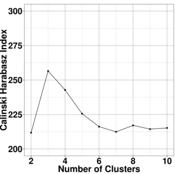
local maximum of the values. For this microbiome data, 3-means clustering

gives the optimal result while 4-means clustering is reasonably good as well. . . 11

2.5

Phylum level relative abundances by subtype from TWA and PCoA. The

left panel shows the barplot of the subject subtype identified by TWA,

and the right panel shows the corresponding barplot for PCoA. For each

subject, relative abundances are aggregated at the phylum level. For each

subtype, the phylum percentages are the means of RA for all OTUs in that

phylum across the subjects in that subtype. Bar heights show number of

subjects in that subtype. The TWA clustering appears to do a better job

of separating subjects with dominant

Proteobacteria

infections from those

with dominant

Firmicutes

infections. . . 12

2.6

Distribution of diagnosis groups in each subtype. The diagnosis groups are

not of equal sizes so in order to compare the distributions of the diagnoses

across subtypes, we calculated the percent of each diagnosis that is

asso-ciated with each subtype. Bars of the same color add up to 100%. All

diagnoses except for Aspiration Pneumonia are equally represented in

Sub-type 1. Aspiration Pneumonia is over represented in SubSub-type 2 where as the

Control group is under represented. The Control group is over represented

2.7

The PCA scree plot of TWA matrix. The scree plot of first sixteen PCs

shows the proportion of total variance attributed to each principal

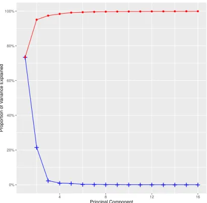
compo-nent (blue line) and the cumulative variance explained (red line). The first

three principal components explain about 96% percent of the variance in

the data. The first seven PCs explain 99.3% of the total variation. The

first sixteen PCs explain 99.9% of the total variation. . . 14

2.8

The PCA scatter plot matrix for TWA. Visualization of the first three

principal components. The points are colored based on their subtype

mem-bership from the 3-means clustering on TWA shown in Figure 2.5. The

plots on the diagonal show the univariate distribution for each of the three

PCs. Off diagonal plots are the pairwise scatter plots. The three clusters

are clearly differentiated in the plot of PC1 versus PC2. . . 14

2.9

Subject cluster labels generated through different approaches and the

cor-responding relative abundance matrix. The left side of the figure shows

three columns. Each column corresponds to an approach; RA, PCoA and

TWA. The rows (subjects) are ordered by cluster labels of TWA results.

The entries are color coded by cluster membership. The plot on the right

shows the RA matrix, where the rows correspond to the colored bar. The

column order is based on the phylogenetic tree. This shows TWA gives the

most useful clustering. . . 15

2.10 The PCA scatter plots based on the RA matrix. Visualization of the first

three principal components of RA. The plots on the diagonal show the

univariate distribution for each of the three PCs. Off diagonal plots are the

pairwise scatter plots. The points in Figure 2.10(a) and Figure 2.10(b) are

colored based on RA clustering and TWA clustering subtypes respectively.

The TWA subtypes are not very related to this view. . . 17

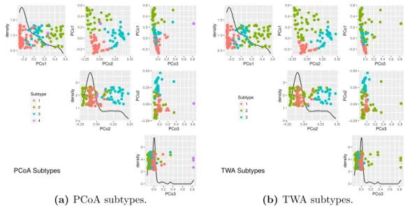
2.11 The scatter plots based on the PCoA scores matrix. Visualization of the

first three principal coordinates of PCoA scores matrix. Format is similar

to Figure 2.10. The points in Figure 2.11(a) and Figure 2.11(b) are colored

based on PCoA clustering and TWA clustering subtypes respectively. PCo1

and PCo2 separates three PCoA subtypes and TWA subtypes. PCoA

Sub-type 4 can be seen as the small set of purple points in the PCo3 dimension

in Figure 2.11(a). . . 17

2.12 Comparison between TWA and other methods by home set abundance odds

ratio (r) and tree distance ratio (d). The left subfigure shows mean NMI

values for representative

d

values and for all values of

r

. The right subfigure

shows mean NMI values for representative

r

values and for all values of

d

.

Error bars represent two times the standard error. From the left subfigure,

TWA is superior to RA except the case

d

= 1 where their performance

are almost the same; TWA dominates PCoA in most cases. PCoA has the

best performance when both

d

and

r

are small. In the right subfigure, for

each value of

r

, NMI of TWA and PCoA converges to the same limit as

d

increases. But TWA converges faster than PCoA. The blue dashed lines

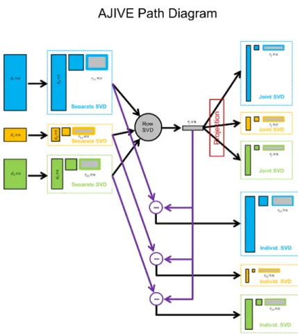
3.1

Flow chart demonstrating the main steps of AJIVE. First low rank

approxi-mation of each data block is obtained on the right. Then in the middle joint

structure between the low rank approximations is extracted using SVD of

the stacked row basis matrices. Finally, on the right, the joint components

(upper) are obtained by projection of each data block onto the joint basis

(middle) and the individual components (lower) come from orthonormal

basis subtraction. . . 28

3.2

Data blocks

X

and

Y

in the toy example . . . 32

3.3

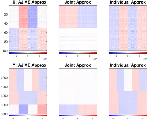
AJIVE approximation of the toy data . . . 33

3.4

The old JIVE approximation of the toy data . . . 37

3.5

Scree plots for the toy data . . . 42

3.6

Principal angle plots between each singular subspace of the signal matrix

A

and its estimator ˜

A

for the toy dataset. Graphics for

X

are on the

upper row, with

Y

on the lower row. The left, middle and right columns

are the under-specified, correctly specified and over-specified signal matrix

rank cases respectively. Each x-axis represents the angle. The y-axis shows

the values of the survival function of the resampled distribution, which are

shown as blue plus signs in the figure. The vertical blue solid line is the

theoretical Wedin bound, showing this bound is well estimated. The

verti-cal black solid line segments represent the principal angles

θ

, . . . , θ

between row(

A

) and row( ˜

A

). The distance between the black and blue

lines reveals when the Wedin bound is tight. . . 46

3.8

Squared singular values in (3.8) and bounds for Step 2 of AJIVE for various

rank choices. The black vertical line segments shows the first ˜

r

∧

r

˜

squared

singular values of

M

in equation (3.8). The values of the survival function

of the random direction bounds are shown as the red circles and the red

dot-dashed line is the 95th percentile of this distribution, which is the random

direction bound. The values of the c.d.f of the Wedin bound are shown as

the blue plus signs and the 5th percentile (blue dashed line) is used for a

prediction interval for the Wedin bound. In the two-block case presented

here this contains the essentially same information as in Figure 3.7. For

the multi-block case it is the major diagnostic graphic. . . 55

3.9

Squared singular value diagnostic graphics for TCGA dataset over various

rank choices. Indicates that there are one joint component among four data

blocks and one joint component among three data blocks. . . 60

3.10 Left: Kernel density estimates of the CNS among GE, CN, RPPA and

mutation. The clear separation among Luminal A versus Her2 and Basal

indicates that these four data blocks share a very strong Luminal A

prop-erty captured in this joint variation component; Right: The CNS from

applying AJIVE to the individual matrices of GE, CN, and RPPA. The

clear separation indicates that these contain a joint variation component

that is consistent with the subtype difference between Basal versus the others. . . 61

3.11 Principal angle diagnostic graphics for Spanish mortality data set over

var-ious rank choices. Provides the rationale of the rank choice, ˜

r

= 3

,

r

˜

= 2. . . 63

3.12 The first block specific joint components of male (left panel) and female

(right panel) contain the common modes of variation caused by the overall

improvement across different age groups, as can be seen from the scores

plots in the right bottom of each panel. The dramatic decrease happened

around the 1950s shown in the columns plots. The degree of decrease varies

over age groups. . . 65

3.13 The second joint components of male (left) and female (right) contain the

common modes of variation driven by the increase in fatalities caused by

automobile penetration and later improvement due to safety improvements.

This can be seen from the scores plots in the right bottom. The loadings

plots show that this automobile event exerted a significantly stronger

im-pact on the 20-45 males. . . 65

3.14 The individual component of male contains the variation driven by the

Spanish civil war which can be seen from the blue circles on the right end

of the right bottom plot. The Spanish civil war mainly affected the young

to middle age males. . . 66

5.1

The graphs of different shrinkage functions under the standard model (5.5).

The horizontal axis represents empirical singular value. The vertical axis

shows shrunken singular values. The blue solid lines show the graphs of the

optimal shrinkage function

η

. The black dashed lines and the purple

dot-dashed lines show the graphs of the optimally tuned soft and hard threshold

functions. The left and right panel shows the case of square and non-square

matrices respectively. This figure is produced by modifying code from the

supplement of Gavish and Donoho (2017). . . 88

5.2

Singular value thresholds for the toy data . . . 89

5.3

Shows the direction specific perturbation angles for different vectors in the

estimated signal row space of

X

, a square matrix introduced in Section 3.1.1

of Chapter 3. The

x

-axis represents angles and the

y

-axis represents the

values of empirical distribution of resampled direction specific perturbation

angles. The vertical blue lines segment on the upper side of each panel show

the value of true direction specific perturbation angle. The blue plus signs

show the empirical distribution of the bootstrap samples of perturbation

angles. The black vertical lines on the lower part of each panel show the

principal angles between the signal space and the estimated signal space.

The vertical cyan dot-dashed lines show the values of the Wedin bound

of the perturbation angle between the signal space and the estimated

sig-nal space. The purple dashed line and solid line show the perturbation

bounds from Theorem 1 and Proposition 1 in Cai et al. (2018) respectively.

Panel 5.3(d) shows the case of rank underestimation, ˆ

r

= 1. In all other

panelsthe signal rank of

X

is correctly specified, i.e. ˆ

r

= 2. The half value

of random angle bound is not shown on this figure since it is larger than

all of these angles. . . 99

5.4

Shows the direction specific perturbation angles for different vectors in the

estimated signal row space of

Y

, a non-square matrix introduced in

Sec-tion 3.1.1 of Chapter 3.In Panel 5.4(a), 5.4(b), 5.4(c) and 5.4(d), the signal

rank of

Y

is correctly specified, i.e., ˆ

r

= 3. In Panel 5.4(e) and 5.4(f), the

signal rank is underestimated, ˆ

r

= 2. . . 101

5.5

Shows the direction specific perturbation angles for different vectors in the

estimated signal row space of

X

when the signal rank, ˆ

r

= 3, is over

estimated. The vertical red dashed lines show the half of the values of

random angle bound. The perturbation bounds from Cai et al. (2018) are

90

°

, which are not useful in this case. . . 102

5.6

Shows the direction specific perturbation angles for different vectors in the

estimated signal row space of

Y

when the signal rank, ˆ

r

= 4, is over

5.7

Scree plots of singular values for data matrices with Gaussian noise. The

x

-axis represents the principal component index, and the

y

-axis shows the

singular values. The black stars show the values of the true signal singular

values. The blue circles and red pluses show the values of the empirical and

shrunken singular values respectively. The horizontal red dashed lines show

the empirical singular value thresholds. The horizontal green dashed lines

show the value

β

in each matrix, which is the cutoff for distinguishable

signal singular values. This shows the singular value shrinkage function

in (5.7) works well in the Gaussian noise case. . . 105

5.8

Scree plot of singular values for data matrices with Student

t

noise. This

shows the singular value shrinkage function in (5.7) works well in the

non-Gaussian noise case. . . 106

5.9

Histogram of empirical singular values. The

x

-axis shows the empirical

singular value and the

y

-axis shows the count of each bin. The vertical

red dashed lines show the empirical singular value thresholds. The vertical

green dashed lines show the theoretical bulk edge, 1 +

√

β

, in each matrix.

This figure shows that the distributions of the empirical singular values

from both Gaussian and non-Gaussian noise matrices follow the generalized

quarter circle law. . . 108

5.10 Direction specific perturbation angles for empirical principal components

for data matrices with Gaussian noise. The black dots show the values

of true perturbation angle. The blue and green dots show the values of

the 95th and 5th percentiles of the resampled perturbation angles. The

horizontal dashed cyan lines show the values of the Wedin bound. The

horizontal red dashed lines show the half values of the random direction

bound. This figure indicates the direction specific estimation algorithm in

Section 5.3 works well for the Gaussian noise case. . . 109

5.11 Direction specific perturbation angles for empirical principal components

CHAPTER 1

Introduction

In the past decade, we are experiencing the era of “big data” and “information explosion”.

Recently many datasets are large-scale not only in the sense of large-sample size and high dimension,

but also in the sense of being multi-source. It is a ubiquitous challenge as well as opportunity for

modern scientific research to integrate the information from disparate data blocks measured on a

common set of experimental subjects. This thesis aims at addressing this challenge by developing

new statistical learning methods for integrative analysis.

Chapter 2 discusses a clustering analysis of a microbiome dataset which incorporates

phyloge-netic information. Modern genomic methods have led to a dramatic increase in the ability to study

a wide variety of microbiomes. In particular, this has enabled precise quantification of various

bacterial species present in a range of different sample types, resulting in many statistical

chal-lenges. For example, discovering disease related pneumotypes of the infected lower lung is difficult

because the lower lung typically has few species of microbes and there is a low level of overlap from

patient-to-patient. This type of sparsity presents a special challenge to standard analysis methods

because it is hard to calculate reliable distances between patients. We address this challenge by

using information from phylogenetic relationships, which results in improved clustering. In our

application to a pneumonia dataset, the method produces statistically distinct, easily described

pneumotypes. It is seen that our pneumotypes are better than those from standard approaches,

using a SWISS score analysis. A simulation study explores the ways in which this new approach

generally performs better than standard methods.

now a fast linear algebra computation. Important mathematical contributions are the use of score

subspaces as the principal descriptors of variation structure and the use of perturbation theory as

the guide for variation segmentation. This leads to an exploratory data analysis method which is

insensitive to the heterogeneity among data blocks and does not require separate normalization.

An application to cancer data reveals different behaviors of each type of signal in characterizing

tumor subtypes. An application to a mortality data set reveals interesting historical lessons.

CHAPTER 2

Finding Community Subtypes On Microbiome Dataset

2.1

Introduction

Modern genomic methods have led to a dramatic increase in the ability to study a wide variety

of microbiomes. An important question is whether or not knowledge of the lower lung microbiome

in patients may aid in the diagnosis, treatment, or prevention of pneumonia (Koenig and Truwit,

2006; Beck et al., 2012; Yamasaki et al., 2013; Dickson et al., 2014; Segal et al., 2014). This

question is approached through determining whether or not there are community subtypes or

pneumotypes. We address the problem of finding pneumotypes by analyzing data from a previously

published study of intensive care unit patients (Bousbia et al., 2012). Most of the subjects in this

dataset were diagnosed with one of several types of pneumonia. For this microbiome dataset, we

focus on

Operational Taxonomic Units

(OTUs), a general biological term including species and

genera. The matrix of the proportions of bacterial OTUs found in each subject’s lung is called the

Relative Abundance

(RA) matrix. Li (2014) gave an overview of high-dimensional data analysis for

microbiome data. As shown in Figure 2.1, in each row of this microbiome data only a few entries

are non-zero, and the distributions of RA over OTUs among different subjects are very diverse.

These features of this microbiome data make it challenging to apply standard analytic methods

because of the difficulty of computing meaningful distances between subjects.

Taxa (OTU)

P

atient

0.00 0.25 0.50 0.75 1.00 proportion

Figure 2.1: Operational taxonomic unit (OTU) relative abundances for the LRI microbiome. Rows

that our approach is better than standard approaches that don’t incorporate information from

the phylogenetic tree. Related microbiome analyses which incorporate relative abundance with

phylogenetic information include Matsen and Evans (2013); Zhao et al. (2015); Chen et al. (2016);

Wu et al. (2016). A standard method that combines phylogenetic distances with RA is Principal

Coordinate Analysis (PCoA) (Gower, 1966), which uses the abundance weighted Unifrac distance

matrix (Lozupone and Knight, 2005).

We carefully study important drivers in a simulation study summarized in Figure 2.2 with the

goal of understanding which method is better over a wide range of potential biological settings. This

shows that TWA is better for a broad range of moderate tree information strength, while PCoA

is the best for a limited set of conditions with very weak tree information (bottom of Figure 2.2).

The black

X

shows the approximate location of this microbiome data, which shows the benefit of

using TWA in this particular case. In a neighborhood of

X, there are many settings where TWA is

much better. The methods perform similarly for very strong tree information, i.e. the upper right

region. A full description is in Section 2.4.

Log odds for relative abundances

Alignment strength

1 1.1 1.2 1.3 1.4 1.5

0 0.5 1 1.5 2 2.5 3 3.5 4

−1.0

−0.5

0.0 0.5 1.0

Figure 2.2: Heat map mutual information comparison of TWA and PCoA. Shades of blue show superior

performance of TWA, with white used for essentially similar cases, and red when PCoA is better. The vertical axis represents the strength of alignment between the phylogenetic tree and clustering in the data. The horizontal axis represents how strongly relative abundances are concentrated in the parts of the phylogenetic tree related to the clusters. This shows a large range of biological settings where TWA is better.

Alonso, 2014a). Section 2.2.1 describes standard statistical clustering algorithms for microbiome

data. Section 2.2.2 discusses Object Oriented Data Analysis (Wang and Marron, 2007; Marron and

Alonso, 2014a), which is a modern framework for approaching complex data challenges and which

provides a viewpoint to address our novel approaches and other approaches to find community

subtypes. Section 2.3 gives the empirical clustering analysis results on the microbiome dataset.

Three distinct pneumotypes with interesting descriptions are identified by the approach we

pro-pose. Compared to standard statistical approaches, our approach gives more balanced and better

statistically separated clustering results. Section 2.4 provides a simulation study to investigate

whether and how the use of phylogenetic tree information improves the identification of clusters.

Section 2.5 discusses the connection between the simulation data and the LRI microbiome data

and concludes with final remarks.

2.2

Methods

2.2.1

Standard clustering algorithms for microbiome analysis

For microbiome analysis, two of the most commonly used algorithms are

k

-means clustering

and mixture modeling.

k-means Clustering

The

k

-means clustering method is a standard clustering approach for

par-titioning a dataset into

k

distinct clusters. Detailed description of its properties can be found in

the book by Kaufman and Rousseeuw (1990). Choosing the best value of

k

is complex. For our

analysis, the Calinski Harabasz Index (Calinski and Harabasz, 1974) is used to estimate the number

of clusters.

Dirichlet Multinomial Mixture Modeling

The Dirichlet Multinomial Mixture Model (DMM,

In their analysis, the data objects are genera-level abundance vectors. Our data from Bousbia et al.

(2012) included only RA values. DMM needs counts as input, so we made an ad hoc conversion to

pseudocounts by multiplying all rows of the RA matrix by an arbitrary value, 100, and rounding

to integers. If the original count data had been available, such an approach could be thought of as

a normalization for sequencing depth.

2.2.2

Object Oriented Data Analysis viewpoint

Object Oriented Data Analysis provides a viewpoint for analyzing complex datasets, such

as curves (Ramsay and Silverman, 2002, 2005), trees (Wang and Marron, 2007; La Rosa et al.,

2012), shapes (Huckemann et al., 2010; Jung et al., 2012) and images (Sen et al., 2008; Lu et al.,

2014). Instead of simply treating data objects as vectors in Euclidean space, an essential idea of

Object Oriented Data Analysis is taking into account their intrinsic information. Object oriented

terminology is useful for understanding these methods for finding community subtypes and how

our new TWA approach relates to them.

RA Vectors As Data Objects

The rows of the RA matrix can be directly represented as

Euclidean vectors on a simplex. Straightforward analysis, say

k

-means clustering, can be applied

to identify subtypes. However, for the microbiome data considered in this paper, both empirical

results in Section 2.3 and simulation results in Section 2.4 show that treating the RA as vectors

does not efficiently represent the subtype structure of subjects because of the high sparsity and

diversity. In particular, only using RA vectors as data objects does not reflect the strong and useful

relationships between the OTUs.

PCoA Scores As Data Objects

PCoA scores computed from the weighted Unifrac distance

weighted Unifrac distance. After computing distances for all pairs of subjects, we get a weighted

Unifrac distance matrix. PCoA then uses multidimensional scaling (Borg and Groenen, 2005) to

produce a coordinate matrix. Community subtypes are next identified by applying, for example,

k

-means clustering to the coordinate matrix produced by PCoA.

TWA Vectors As Data Objects

We propose TWA as a novel data object that combines RA

and phylogenetic tree information. TWA is the abundance weighted by the cophenetic distance

matrix (Sokal and Rohlf, 1962) of OTUs in the phylogenetic tree, where cophenetic distance is

the sum of the branch lengths traversed between two leaves in the phylogenetic tree. Denote the

cophenetic distance matrix and RA matrix as

D

and

X

respectively. The matrix

X

has subjects

as rows and OTUs as columns. Then, the Tree Weighted Abundance is calculated as

TWA =

X

·

D.

The rows of TWA can serve as the data objects for various clustering approaches, such as

k

-means

clustering. This new data object, which incorporates phylogenetic tree information with RA, is in

the spirit of weighted UniFrac distances. Weighted UniFrac, however, measures distances between

subjects, whereas TWA can be best thought of as a transformation of RA. Because of the weighting

scheme, subjects with OTUs that are phylogenetically related will be close in TWA space even when

there is no overlap in OTUs, which is essentially important for data of the type shown in Figure 2.1.

2.3

Analysis of the real microbiome data

In this section we describe the application of TWA on the real microbiome data.

2.3.1

Data description and processing

study that allowed an unusually high level of resolution. Most of the OTUs, consequently, could be

identified at the species-level using BLAST against GenBank. Relative abundance estimates were

provided by the authors.

The initial data included 157 OTUs.

We selected for analysis only taxonomic units with

sufficient representation in GenBank to include in the calculation of a phylogenetic tree. In a

few cases, we aggregated OTUs at the genus level in order to have sufficient reference genomes

for accurate calculation of the tree. In total, 121 OTUs, mostly at the species level, had enough

reference genomes available for phylogenetic analysis.

We restricted our analysis to subjects that had bacteria identified in their sample. Final data

included 124 pneumonia subjects and 13 controls. We verified that the filtered data had about the

same level of sparsity as the original. The mean number of OTU’s per subject before filtering was

3.6 (s.e.=0.24) and after filtering was 3.2 (s.e.=0.20). We calculated the Bray-Curtis diversity (Bray

and Curtis, 1957), a measure of the dissimilarity between a pair of subjects, of all pairs of subjects

before and after filtering. For each subject we calculated the median value all pairs. The mean

value across subjects was 1.0 (s.e.=0) for both the original and filtered datasets.

2.3.2

Computing the phylogenetic tree

Figure 2.3: The unrooted phylogenetic tree computed by PhyloPhlAn. Tips are labeled with the OTU names. Tips are colored based on the phylum identification from NCBI. In general, this tree is consistent with the NCBI taxonomy.

2.3.3

k-means clustering on TWA

For our analysis, we used the R-package

fpc

(Hennig, 2015). This implements a standard

k

-means algorithm which initializes the -means several times by using seeds that are randomly selected

data points. Applying

k

-means clustering on TWA for values of

k

ranging from 2 to 10, as seen

in Figure 2.4, the Calinski Harabasz index (Calinski and Harabasz, 1974) was highest for three

clusters so all subsequent analysis will be based on 3-means clustering.

● ●

●

●

●

● ●

● ●

200

225

250

275

300

2

4

6

8

10

Number of Clusters

Calinski Harabasz Inde

x

Figure 2.4: Calinski Harabasz index values for different numbers of clusters fork-means on TWA. Larger

value of Calinski Harabasz index indicates a better separated clustering results.The optimal clustering should be given by the first local maximum of the values. For this microbiome data, 3-means clustering gives the optimal result while 4-means clustering is reasonably good as well.

appearing most prominently. These three subtypes represent different types of infections which

make biological sense and are reasonably balanced. The right panel shows direct comparison of the

clustering by PCoA, and will be discussed in Section 2.3.6.

2.3.4

Description of TWA subgroups based on diagnosis

90.2%

82.5% 11.9%

10.0% 47.7% 28.2% 13.9%

0 20 40 60 80

Subtype 1 Subtype 2 Subtype 3

Subject subtype identified by TWA

Siz

e of subtype

11.3% 83.1%

87.1% 7.4%

5.8% 45.2% 34.8% 13.6%

100.0% 0

20 40 60 80

Subtype 1 Subtype 2 Subtype 3 Subtype 4

Subject subtype identified by PCoA

Siz

e of subtype

Actinobacteria Bacteroidetes Firmicutes Proteobacteria Other

Figure 2.5: Phylum level relative abundances by subtype from TWA and PCoA. The left panel shows the

barplot of the subject subtype identified by TWA, and the right panel shows the corresponding barplot for PCoA. For each subject, relative abundances are aggregated at the phylum level. For each subtype, the phylum percentages are the means of RA for all OTUs in that phylum across the subjects in that subtype. Bar heights show number of subjects in that subtype. The TWA clustering appears to do a better job of separating subjects with dominantProteobacteriainfections from those with dominantFirmicutesinfections.

2.3.5

Principal components visualization

In order to visualize the clustering results in the TWA space, PCA is applied to the TWA. The

first three principal components explain a large amount of the variation, about 97.4%, and the first

PC explains 73%. The corresponding scree plot is provided in Figure 2.7.

0% 20% 40% 60% 80%

Subtype 1 Subtype 2 Subtype 3

P

er

cent of Dia

gnosis Gr

oup Assigned to Eac

h Subtype

Diagnosis

Control AP CAP NVHAP VAP

Figure 2.6: Distribution of diagnosis groups in each subtype. The diagnosis groups are not of equal sizes

+

+

+ + + + + + + + + + + + + +

4 8 12 16

Principal Component

Propor

tion of V

ar

iance Explained

Figure 2.7: The PCA scree plot of TWA matrix. The scree plot of first sixteen PCs shows the proportion of

total variance attributed to each principal component (blue line) and the cumulative variance explained (red line). The first three principal components explain about 96% percent of the variance in the data. The first seven PCs explain 99.3% of the total variation. The first sixteen PCs explain 99.9% of the total variation.

● ● ● ● ● ● ● ● ●●●●●●●●●●●●●● ●●●●●●●● ●●●●●●●●●●●●●●●●●●●●●●●●●●●● ●●●● ● ●● ●● ● ●●● ●●● ●● ●●● ●●●● ●●●●● ●●●●●● ● ●●●● ●● ●● ● ● ● ● ●● ●●●●● ●●●●●●●●●●●●●●●●●●●●●●● 0.008 0.012 0.016

−20 0 20

PC1 density ● ● ● ● ● ● ● ● ● ● ● ● ●● ● ● ● ● ● ● ● ● ● ● ● ● ● ● ● ● ● ● ● ● ● ● ● ● ● ● ● ● ● ● ● ● ● ● ● ● ● ● ● ● ● ● ● ● ● ● ● ●● ● ● ● ● ● ● ● ● ● ● ● ● ● ● ● ● ● ● ● ●● ● ● ● ● ● ● ● ● ● ● ● ●● ●● ● ● ● ● ● ● ● ● ● ● ● ● ● ● ● ● ● ● ● ● ● ● ● ● ● ● ● ● ● ● ● ● ● ● ● ● ● ● −20 0 20

0 20 40

PC2 PC1 ● ● ● ● ● ● ● ● ● ● ● ● ● ● ● ● ● ● ● ● ● ● ● ● ● ● ● ●● ● ● ● ● ● ● ● ● ● ● ● ● ● ● ● ● ● ● ● ● ● ● ● ● ● ● ● ● ● ● ● ● ● ● ● ● ● ● ● ● ● ● ● ● ● ● ● ● ● ● ● ● ● ●● ● ● ● ● ● ● ● ● ● ● ●●●● ● ● ● ● ● ● ● ● ● ● ● ● ● ● ● ● ● ● ● ● ● ● ● ● ● ● ● ● ● ● ● ● ● ● ● ● ● ● ● −20 0 20

−5 0 5 10

PC3 PC1 ● ● ● ● ●● ●●● ● ●●●●●●●●●●●●●●●●●●●●●●●●●● ●●●●●●●●●●●●●●●● ●●● ● ●●●●●●●●●●●●●●●●●●●●●●●●●●●●●●●●●●●●●●●●●●●●●●●●●●●●●●●●●●●●●●●●●●●●●●● ●●●●●●●●●● 0.00 0.02 0.04 0.06

0 20 40

PC2 density ● ● ● ● ● ● ● ● ● ● ● ● ● ● ● ● ● ● ● ● ● ● ● ● ● ● ● ● ● ● ● ● ● ● ● ● ● ● ● ● ● ● ● ●● ● ● ● ● ● ● ● ● ● ● ● ● ● ● ● ● ● ● ● ● ● ● ● ● ●● ● ● ● ● ● ● ● ● ● ● ● ●● ● ● ● ● ● ● ● ● ● ● ●●●● ●● ● ● ● ● ● ● ● ● ● ● ● ● ● ● ● ● ● ● ●● ● ● ● ● ● ● ● ● ● ● ● ● ● ● ● ● ● 0 20 40

−5 0 5 10

PC3 PC2 ● ● ● ●● ● ● ●●●● ●● ● ●●● ● ● ● ●● ● ● ●●● ● ● ● ●●●●●●●●●●●●●●●● ●●●●●●●●●●●● ●●●●●● ●●●●●●●●●●●●●●●●●●●●●●●●●●●●●● ●● ●●●●●●●●●●●●●●●●●●●●●●● ●●●●●●●●●●●●●●● ● ● ● 0.000 0.025 0.050 0.075 0.100

−5 0 5 10

PC3 density TWA Subtypes ● ●● ●● ●● ● ●●●● ● ●●● ● ●● ●●● ● ●● ●●●● ● ● ● ●●● ●●● ● ● ● ●● ● ● ●● ● ● ●● ●● ●● ●● ● ●●● ● ●● ●●● ●●●●●●● ● ● ● ● ● ●●●●●●● ● ●●●●● ●● ● ● ● ● ●●● ● ● ●●● ● ●● ●●● ●● ●●●● ● ● ● ● ● ●● ● ●●●●●●●● ● ●● Subtype ● ● ● 1 2 3

Figure 2.8: The PCA scatter plot matrix for TWA. Visualization of the first three principal components.

2.3.6

Comparison of results from other approaches

Clustering results based on the three approaches are shown in Figure 2.9. Applying the DMM

modeling to the taxa level RA matrix does not identify any subtypes so these results are not shown

in the figure. Applying

k

-means clustering to the RA matrix identifies two subtypes based on the

Calinski-Harabasz index. Subjects in the smaller of the two clusters have a single dominant OTU

(shown as red in the left column of the colored bar, and as a short vertical line segment in the RA

matrix). Subjects in the other cluster are simply all the rest. As shown in the right two columns

of the colored bar, clustering based on the PCoA score matrix gives results that are fairly similar

to TWA. Subtype 1 in TWA remains in the first subtype of PCoA. In contrast, PCoA distributes

members of TWA Subtype 2 among its other subtypes. An interesting question is which phyla have

left the TWA Subtype 2 to join the others. This is answered by the right panel of Figure 2.5, which

shows the phylum level RA by subtype from the PCoA approach. Note that both

Proteobacteria

and

Firmicutes

have been moved to PCoA Subtype 1. Furthermore,

Firmicutes

have also been

moved to PCoA Subtype 3 and to the new PCoA Subtype 4. Finally notice the overall subtype

sizes are much less balanced for PCoA.

RA PCoATWA

Method

Subject

Subtype

1 2 3

4 _0.000.25

0.50 0.75 1.00

proportion

Figure 2.9: Subject cluster labels generated through different approaches and the corresponding relative

Since

k

-means clustering gives different numbers of clusters on different data objects, in

or-der to make a complete comparison we evaluate 2-means, 3-means and 4-means clustering on all

three data objects. SWISS (Cabanski et al., 2010) scores and Calinski-Harabasz index values, two

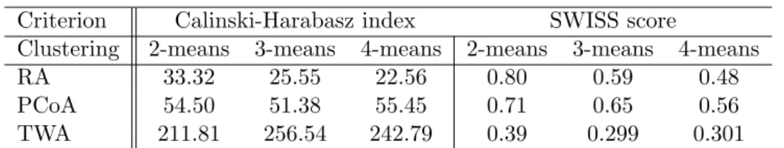
nonparametric criteria for clustering evaluation, are provided in Table 2.1 for all three methods.

Large values of the Calinski-Harabasz index and small values of the SWISS score indicate better

separated clusters. As shown in Table 2.1, 3-means clustering based on TWA gives the best results

among all approaches. PCoA is inferior to TWA, and overall is somewhat better than clustering

directly on RA values.

Table 2.1: Calinski-Harabasz index values and SWISS scores from k-means clustering on different data

objects. This shows much better clustering performance for TWA.

Criterion

Calinski-Harabasz index

SWISS score

Clustering

2-means

3-means

4-means

2-means

3-means

4-means

RA

33.32

25.55

22.56

0.80

0.59

0.48

PCoA

54.50

51.38

55.45

0.71

0.65

0.56

TWA

211.81

256.54

242.79

0.39

0.299

0.301

Principal components visualization of RA and PCoA clustering results

Visualization of

RA and PCoA clustering results, analagous to Figure 4 based on TWA, are shown here. For the RA

matrix, the first three Principal Component scatter plots colored by RA and TWA clustering results

are shown in Figure 2.10(a) and Figure 2.10(b) respectively. Note that the only difference between

Figure 2.11(a) and Figure 2.11(b) is the coloring of the points. PC1 shows a bimodal structure,

which separates RA Subtype 1 (red) and RA Subtype 2 (green). This shows how

k

-means found

those clusters. PC2 and PC3 don’t show a clear subtype view. TWA subtypes do not follow the

data structure in these scatter plots.

●● ● ● ● ● ●●●●●●● ●● ● ● ● ● ●●●●●●●●●●●●●●●●●●●●●●●●●●●●●●●●●●●●●●●●●● ●● ●●●●●●● ● ●●●●●●●●●●●●● ● ● ●● ●●●●●●●●●●●●●●●●●●●●●●●●●●●●●●●●●●●● ●●●●●●●● ●●●●● 0 5 10 15 20

−0.3 0.0 0.3 0.6 0.9

PC1 density ● ●● ● ●● ●● ● ● ●● ● ● ●● ● ● ● ● ●● ● ● ● ●●●● ● ● ● ● ● ● ● ● ● ● ● ● ● ● ● ● ● ● ●●● ● ● ● ● ●● ● ●● ● ● ● ●● ●●●●● ● ● ● ●● ●●●●●●●●● ● ● ● ● ● ● ● ● ● ● ●● ● ● ●● ● ● ● ●●●●●●● ● ● ● ● ● ● ● ●● ●● ●●●● ● ● ● ● ● ● ● ●● ● ● ●● −0.3 0.0 0.3 0.6 0.9 0.0 0.5 PC2 PC1 ● ●● ● ●●●● ● ●● ● ● ● ●● ●● ● ● ● ● ● ● ●●●● ● ● ● ● ● ● ● ● ●● ● ● ● ● ● ● ● ● ● ●●● ● ● ● ● ● ● ● ● ●●●● ● ● ●●●●● ● ● ●● ● ● ● ● ● ●●●●●● ● ● ● ● ● ● ●● ● ● ●●●● ● ● ●● ●●●● ●●● ● ● ● ● ● ● ● ●● ●● ●●●●● ● ● ● ● ● ● ● ● ● ● ●● −0.3 0.0 0.3 0.6 0.9

0.00 0.25 0.50 0.75

PC3 PC1 ● ●●● ●● ●●●●●●●●●● ● ●●●●●●●●●●● ● ● ●● ●●●●●●●●●●●●●●●●●●●●●●●●●●●●●●●●●●●●●●●●●●●●●●●●●●●●●●●●●●●● ● ●●● ●●●●●●●●●●●●● ●●●●●●●●●●●●●●●●●●●●●● ●●● ● ●● 0 5 10 0.0 0.5 PC2 density ● ●● ● ●● ● ● ● ● ● ●●● ●● ●● ● ● ● ● ● ● ● ●● ● ● ● ● ● ● ● ● ● ●● ●● ● ● ● ● ● ● ● ●●● ● ● ● ●●●● ● ●●●● ● ● ●●●●● ● ● ●● ● ● ● ● ● ●●● ● ● ● ● ● ● ● ● ● ●●●● ●● ● ● ● ● ● ● ●●●● ●●●● ● ● ● ● ● ● ●● ●● ● ● ● ●● ● ● ● ● ● ● ● ● ● ● ●● 0.0 0.5

0.000.250.50 0.75

PC3 PC2 ● ●●● ●●●●●●●●●● ●●●●●●●●●●●●●●● ● ● ● ●● ●●●●●●● ●●●●●●●●●●●●●●●●● ●●●● ● ● ● ●● ●●●●●●●●●● ● ●●●● ●●●●●●●●●● ●● ●●●●●●●●●●●●●●●●●●●●●●● ●●●●●●●●●●●●●●●●●● ●● 0 2 4 6

0.00 0.25 0.50 0.75

PC3 density RA Subtypes ● ● ●● ● ● ● ●● ● ● ●●● ● ● ● ● ● ● ● ● ●● ● ● ● ● ● ● ● ●● ● ●● ● ● ●●●● ● ● ●● ● ● ● ● ●● ● ● ●● ● ● ● ● ● ● ● ● ● ● ● ● ● ● ● ● ● ● ● ● ● ● ● ● ● ● ● ● ● ●●● ● ● ● ●● ● ● ● ● ● ● ● ● ● ● ● ● ● ● ● ● ● ● ●● ●● ● ● ● ● ● ● ● ● ● ●●● ● ● ● ● ● ● ● ● ● ● Subtype ● ● 1 2

(a)RA subtypes.

●● ● ● ● ● ●●●●●●● ● ● ● ● ● ●●●●●●●●●●●●●●●●●●●●●●●●●●●●●●●●●●●●●●●●●●● ●● ●●●●●●● ● ●●●●●●●●●●●●● ● ● ●● ●●●●●●●●●●●●●●●●●●●●●●●●●●●●●●●●●●●●●●●●●●●● ●●●●● 0 5 10 15 20

−0.3 0.0 0.3 0.6 0.9

PC1 density ● ●● ● ● ● ●● ● ● ●● ● ● ●● ● ● ● ● ● ● ● ● ●●●●● ● ● ● ● ● ● ● ● ● ● ● ● ● ● ● ● ● ● ●●● ● ● ● ● ●● ●●● ● ● ● ●● ●●●●● ● ● ● ●● ●●●●●●●●● ● ● ● ● ● ● ● ● ● ● ● ● ● ● ●● ● ● ● ●●●●●●● ● ● ● ● ● ● ● ●● ●● ●●●● ● ● ● ● ● ● ● ●● ● ● ●● −0.3 0.0 0.3 0.6 0.9 0.0 0.5 PC2 PC1 ● ●● ● ●●●● ● ●● ● ● ● ●● ●● ● ● ● ● ● ● ● ●● ● ● ● ● ● ● ● ● ● ●● ● ● ● ● ● ● ● ● ● ●●● ● ● ● ● ● ● ●● ●●●● ●● ●●●●● ● ● ●● ● ● ● ● ● ●●●●●● ● ● ● ● ● ● ●● ● ● ●●●● ● ● ●● ●●●● ●●● ● ● ● ● ● ● ● ●● ●● ●●●●● ● ● ● ● ● ● ● ● ● ● ●● −0.3 0.0 0.3 0.6 0.9

0.00 0.25 0.50 0.75

PC3 PC1 ● ● ●● ●● ●●●●● ●●●●● ● ● ●●● ●●●●●●● ● ● ●●●●●●●●●●●●●●●●●●●●●●●● ●●●●●●●●●●●●●●●●●●●●●●●●●●●●●●●●●●●●●● ● ●●● ●●●●●●●●●●●●●●●●●●●●●●●●●●●●● ●●●●●● ●●● ● ●● 0 5 10 0.0 0.5 PC2 density ● ●● ● ●● ● ● ● ● ● ●●● ●● ●● ● ● ● ● ● ● ● ●● ● ● ● ● ● ● ● ● ● ●● ●● ● ● ● ● ● ● ●●●● ● ● ● ●●●● ● ●●●● ●● ●●●●● ● ● ●● ● ● ● ● ● ●●● ● ● ● ● ● ● ● ● ● ●●●● ●● ● ● ●● ● ● ●●●● ●●●● ● ● ● ● ● ● ●● ●● ● ● ● ●● ● ● ● ● ● ● ● ●● ● ●● 0.0 0.5

0.000.25 0.500.75

PC3 PC2 ● ●●● ●●● ●●●● ●●● ●● ●●●●●●●●●●●● ● ● ● ● ●● ●●● ●●●●●●●●●●●●●●●●●●●●● ●●●● ●● ●●●●● ●●●●●●●●●●●● ●●●●●●●●●●●● ● ●●●●●●●●●●●●●●●●●●●●●●●●●●●●●●●●●●●●●●●●● ●● 0 2 4 6

0.00 0.25 0.50 0.75

PC3 density TWA Subtypes ● ● ●● ● ● ● ● ● ● ● ●●● ● ● ● ● ● ● ● ● ● ● ● ● ● ● ● ● ● ● ● ● ●● ● ● ●●●● ● ● ● ● ● ● ● ● ●●● ●●● ● ● ● ● ● ● ● ● ● ● ● ● ● ● ● ● ● ● ● ● ● ● ● ● ● ● ● ● ● ●●● ● ● ● ●● ● ● ● ● ● ●● ● ● ● ● ● ● ● ● ●● ● ●● ●● ● ● ● ● ● ● ● ● ● ●●● ●● ● ● ● ● ● ● ● ● Subtype ● ● ● 1 2 3

(b) TWA subtypes.

Figure 2.10: The PCA scatter plots based on the RA matrix. Visualization of the first three principal

components of RA. The plots on the diagonal show the univariate distribution for each of the three PCs. Off diagonal plots are the pairwise scatter plots. The points in Figure 2.10(a) and Figure 2.10(b) are colored based on RA clustering and TWA clustering subtypes respectively. The TWA subtypes are not very related to this view.

between PCoA and TWA clusterings. A new small subtype, PCoA Subtype 4 (purple), appears in

PCo3.

−0.2 0.0 0.2 0.4 0.6

PCo1 density ● ● ● ● ● ● ● ● ● ● ● ● ●● ● ● ● ● ● ● ● ● ● ● ● ● ● ●● ● ● ● ● ● ● ● ● ● ● ● ● ● ● ●● ● ● ● ● ● ● ● ● ● ● ● ● ● ● ● ● ● ● ● ● ● ● ● ● ● ● ● ● ● ● ● ● ● ● ● ● ● ● ● ● ● ● ● ● ● ● ● ● ● ● ● ●●● ● ● ● ● ● ● ● ● ● ● ● ● ● ● ● ● ● ● ● ●● ● ● ● ● ● ● ●● ● ● ● ● ● ● ●● ● −0.2 0.0 0.2 0.4 0.6

−0.25 0.00 0.25 0.50

PCo2 PCo1 ● ● ● ● ● ● ● ● ● ● ● ● ● ● ● ● ● ● ● ● ● ● ● ● ● ● ● ●● ● ● ● ● ● ● ● ● ● ● ● ● ● ● ● ● ● ● ● ● ● ● ● ● ● ● ● ● ● ● ● ● ● ● ● ● ● ● ● ● ● ● ● ● ● ● ● ● ● ● ● ● ● ●● ● ● ● ● ● ● ● ● ● ● ● ● ● ● ● ● ● ● ● ● ● ● ● ● ● ● ● ● ● ● ● ● ● ●●● ● ● ● ● ● ● ●● ● ● ● ● ● ● ● ● ● −0.2 0.0 0.2 0.4 0.6

0.00.20.4 0.60.8

PCo3 PCo1 ● ● ● ●● ● ●●● ● ●●●●●●●●●●●●●●●● ●●●●●●●●●●● ●●●●●●●●●●●●●●●●●●●●●●●●●●●●●●●● ● ● ● ●●●● ● ● ● ●● ● ● ●●●●●●●●●●●●●●●●●●●●●●●●●●●●●●●●●● ●●●●●●●●●●●●●●●●●●●● 0 1 2 3

−0.25 0.00 0.25 0.50

PCo2 density ● ● ● ●● ● ● ●● ● ● ● ● ● ● ● ●● ● ● ● ● ● ● ● ● ● ● ● ● ● ● ● ●●● ● ● ● ● ● ● ● ● ●● ● ● ● ● ● ● ● ● ● ● ● ● ● ● ● ● ● ● ● ● ● ● ● ● ● ● ● ● ●● ● ● ● ● ● ● ●● ● ● ● ● ● ● ● ● ● ● ● ● ● ● ● ● ● ● ● ● ● ● ● ● ● ● ● ● ● ● ● ● ●● ● ● ● ● ● ● ● ● ●● ● ● ● ● ● ● ● ● ● −0.25 0.00 0.25 0.50

0.00.20.40.60.8

PCo3 PCo2 ● ●●●●● ●●●●● ●●● ●●●●●●●●●●●●●●●●●●●●●●●●●●●●●●●●●●●●●●●●●●●●●●●●●●●●●●●●●●●● ●● ●●●●●●●●●●●●●●●●●●●●●●●●●●●●●●●● ● ●● ●●●●●●●●●●●●●●●●●●●●●●●● ● ● 0 2 4 6

0.0 0.2 0.4 0.6 0.8

PCo3 density PCoA Subtypes ● ● ● ● ● ●● ● ●●●● ● ●● ● ● ●● ●● ● ● ●● ●● ● ● ● ● ● ● ●● ● ●● ● ● ● ● ● ● ● ● ● ● ● ●● ●● ● ● ●● ● ●● ● ● ●● ●● ● ● ●●●●●● ●●● ●● ●●●●●●● ● ●●● ● ● ●● ● ● ● ● ●●●●● ●● ● ● ●● ●●● ● ● ● ●● ● ● ●●●● ●● ● ● ●●●● ● ● ● ● ●● Subtype ● ● ● ● 1 2 3 4

(a)PCoA subtypes.

● ● ● ● ● ● ● ● ●●●● ●●●● ●●● ●●● ● ●●●● ●● ● ●● ●●●● ●● ● ● ● ● ● ●● ●●●●● ● ●●●● ● ● ● ●●●●● ●● ● ● ● ●●●● ●● ●● ●●● ● ● ●●●●● ● ● ●●● ● ● ● ● ● ● ● ● ●● ● ● ●●● ● ●● ● ● ● ● ● ●● ●●●●●●● ●● ● ●● ●●●●● ● ●● ● 0.5 1.0 1.5

−0.2 0.0 0.2 0.4 0.6

PCo1 density ● ● ● ● ● ● ● ● ● ● ● ● ●● ● ● ● ● ● ● ● ● ● ● ● ● ● ●● ● ● ● ● ● ● ● ● ● ● ● ● ● ● ●● ● ● ● ● ● ● ● ● ● ● ● ● ● ● ● ● ● ● ● ● ● ● ● ● ● ● ● ● ● ● ● ● ● ● ● ● ● ● ● ● ● ● ● ● ● ● ● ● ● ● ● ●●● ● ● ● ● ● ● ● ● ● ● ● ● ● ● ● ● ● ● ● ●● ● ● ● ● ● ● ●● ● ● ● ● ● ● ●● ● −0.2 0.0 0.2 0.4 0.6

−0.25 0.00 0.25 0.50

PCo2 PCo1 ● ● ● ● ● ● ● ● ● ● ● ● ● ● ● ● ● ● ● ● ● ● ● ● ● ● ● ● ● ● ● ● ● ● ● ● ● ● ● ● ● ● ● ● ● ● ● ● ● ● ● ● ● ● ● ● ● ● ● ● ● ●● ● ● ● ● ● ● ● ● ● ● ● ● ● ● ● ● ● ● ● ●● ● ● ● ● ● ● ●● ● ● ● ● ● ● ● ● ● ● ● ● ● ● ● ● ● ● ● ● ● ● ● ● ● ●●● ● ● ● ● ● ● ●● ● ● ● ● ● ● ● ● ● −0.2 0.0 0.2 0.4 0.6

0.00.20.4 0.60.8

PCo3 PCo1 ● ● ● ●● ● ●●● ● ●●●●●●●●●●●●●●●●●●● ●●●●●●●●●● ●●●●●●●●●●●●●●●●●●●●●●●●●●●●●●●●●●●●●●● ● ●● ● ● ●●●●●●●●●●●●●●●●●●●●●●●●●●●●●●●●●● ●●●●●●●●●●●●●●●●●●●● 0 1 2 3

−0.25 0.00 0.25 0.50

PCo2 density ● ● ● ●● ● ● ●● ● ● ● ● ● ● ● ●● ● ● ● ● ● ● ● ● ● ● ● ● ● ● ● ●●● ● ● ● ● ● ● ● ● ●● ● ● ● ● ● ● ● ● ● ● ● ● ● ● ● ● ● ● ● ● ● ● ● ● ● ● ● ● ● ● ● ● ● ● ● ● ●● ● ● ● ● ● ● ● ● ● ● ● ● ● ● ● ● ● ● ● ● ● ● ● ● ● ● ● ● ● ● ● ● ●● ● ● ● ● ● ● ● ● ●● ● ● ● ● ● ● ● ● ● −0.25 0.00 0.25 0.50

0.00.20.40.60.8

PCo3 PCo2 ●●●●●● ●●●●● ●●● ●●●●●●●●●●●●●●●●●●●●●●●●●●●●●●●●●●●●●●●●●●●●●●●●●●●●●●●●●●●● ●● ●●●●●●●●●●●●●●●●●●●●●●●●●●●●●●●● ● ●● ●●●●●●●●●●●●●●●●●●●●●●●● ● ● 0 2 4 6

0.0 0.2 0.4 0.6 0.8

PCo3 density TWA Subtypes ● ● ● ● ● ●● ● ●●●● ● ●●● ● ●● ●● ● ● ●● ●● ● ● ● ● ● ● ●● ● ●● ● ● ● ●● ● ● ● ● ● ● ●● ●● ● ● ●● ● ●● ● ● ●● ●● ● ● ●●●●●● ●●● ●● ●●●●●●● ● ●●●●● ●● ● ● ● ● ●●●●● ●● ● ● ●● ●●● ● ● ●●●●●●●●● ●● ● ● ●●●● ● ● ● ● ●● Subtype ● ● ● 1 2 3

(b) TWA subtypes.

Figure 2.11: The scatter plots based on the PCoA scores matrix. Visualization of the first three principal

coordinates of PCoA scores matrix. Format is similar to Figure 2.10. The points in Figure 2.11(a) and Figure 2.11(b) are colored based on PCoA clustering and TWA clustering subtypes respectively. PCo1 and PCo2 separates three PCoA subtypes and TWA subtypes. PCoA Subtype 4 can be seen as the small set of purple points in the PCo3 dimension in Figure 2.11(a).

information more effectively than PCoA. The three subtypes of subjects generated by TWA are

statistically separated, well balanced, and are also easy to explain in terms of phyla.

2.4

Simulation study

The analysis in Section 2.3 indicates that TWA is a preferable approach to clustering analysis

on this microbiome data. The empirical results in Section 2.3 also indicate that in each subtype

of subjects the RAs concentrate on some specific OTUs, which are close in the phylogenetic tree.

We use a simulation study to study potential biological contexts beyond this case. We generate

OTU RA matrices that have the similar sparse features of the lung microbiome data and vary the

connections between the subtype structure and the phylogenetic tree structure. The four clustering

approaches in Section 2.2 are compared. Our study makes clear situations in which each analysis

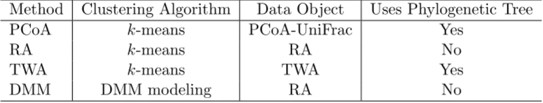
strategy is the best choice.

In our simulation study, the four analysis methods in Section 2.2 are compared. Applying

DMM modeling on RA

(DMM) and

k

-means clustering on PCoA scores of Unifrac

(PCoA) are popular approaches to microbiome analysis in the literature.

Applying

k

-means

clustering on RA

(RA) is a straightforward clustering approach. Applying

k

-means clustering

on TWA

(TWA) is the novel approach we propose. These methods are summarized in Table 2.2.

Table 2.2: Four methods of microbiome clustering analysis.

Method

Clustering Algorithm

Data Object

Uses Phylogenetic Tree

PCoA

k

-means

PCoA-UniFrac

Yes

RA

k

-means

RA

No

TWA

k

-means

TWA

Yes

DMM

DMM modeling

RA

No

2.4.1

Simulation settings

of their probability distribution over 100 OTUs, which are divided into five sets of sizes 10, 20, 20,

30, and 20 respectively. In this design, each group of subjects is assumed to be strongly associated

with a specific set of OTUs. For simplicity of notation, a subject in Group 1 is most likely to have

OTUs observed from Set 1, a subject from Group 2 is most likely to have OTUs observed from Set

2, and so on. We call Set 1 the

home

set of Group 1, etc. Set 5 is not associated with any groups

of subjects and is included to make the cluster problem more challenging.

We define the

home set abundance odds ratio,

r

, as the odds ratio of observing an OTU from

the home set versus observing an OTU from any of the other four sets. For this simulation,

r

ranges

from 1 to 16. The value

r

= 1 is the minimum value by definition of home set. The value

r

= 16

is a case where all methods perform well.

Two of the analysis methods require a phylogenetic tree. We generate simple phylogenetic trees

where the cophenetic distances between any two OTUs from the same set are fixed at 1 and the

distances between any two OTUs from different sets are fixed at

d

. We call

d

the

tree distance

ratio. The case

d <

1 is not considered because then the phylogenetic tree would put the OTUs

in the same set far from each other. The minimum considered value

d

= 1 is the case where the

phylogenetic tree has no information about home sets. The maximum value

d

= 1

.

5 is a case where

all methods perform well.

In summary, the home set abundance odds ratio,

r

, represents the strength of the connections

between the subtype structure of subjects and the home set taxa RA values. The tree distance ratio,

d

, represents the strength of the alignment between subtype structure of subjects and the

phylo-genetic tree. Values of these two parameters, which cover a broad range of association strengths,

are intended to generate conditions that will help us differentiate among the analysis methods. For

each value of

r

, 200 datasets are generated. For each dataset, a phylogenetic tree is generated for

each value of

d

.

2.4.2

Data generating model

In this section we introduce the data generating model in the simulation study. We intend to

generate RA datasets that resemble the sparsity in the real microbiome data. In particular