CUSTOMER ORDER FORECASTING IN SUPPLY CHAINS A SIMULATION STUDY

(1)

CUSTOMER ORDER FORECASTING IN SUPPLY CHAINS

A SIMULATION STUDY

Balaji Janamanchi

Texas A&M Int’l University, Division of International Business and Technology Studies College of Business Administration, 5201, University Boulevard, Laredo, Texas 78041,

Phone: (956)326-2537 Fax : (956)326-2494, Email: [email protected]

James R. Burns, P.E., CIRMP

6

P

Texas Tech University, Rawls College of Business Administration ISQS area, P.O.Box 42101, Lubbock, Texas 79409-2101 Phone: (806)742-1547 Fax: (806)742-3193, Email: [email protected]

ABSTRACT

System dynamics is the preferred methodology for gaining a deeper and better understanding of complex systems, both for social or business systems, that are fraught with unavoidable delays and complex feedback loops. Order information distortion in supply chains is a major concern that causes the well-known bullwhip effect. Enterprise-wide visibility through IT and extranet data access between trading partners is an effective measure to address the information distortion and thereby to thwart the propagation of the bullwhip effect. Other strategies, such as dynamic order forecasting, ordering policies that do not entail the immediate replacement of used safety stocks, expanded workweek to absorb the surges in production demand may prove to be useful complements to the strategy of information visibility to enhance the benefits of information visibility in supply chains. The purpose of this paper is to study these complementary strategies and their effectiveness along with enterprise-wide visibility, in the mitigation of the bull-whip effect.

Introduction

There is no denying the fact that many well-intended managerial decisions in business systems fail to yield their expected results. Managers often ascribe these failures to unintended side effects of the decisions or changed circumstances. Limitations of typical human intuition being what they are, we all accept these side effects as a feature of reality. However, Sterman (2000) points out that, “Side effects are not a feature of reality but a sign that our understanding of the system is narrow and flawed.”

Supply chains are complex business systems that behave badly when typical managerial practices are applied to them. Based on the “nature of inputs and objective of study,” Beamon (1998) has identified four main categories of models used in analyzing and designing supply chains as follows,

“(1) deterministic analytical models, in which the variables are known and specified, (2) stochastic analytical models, where at least one of the variables is

(2)

unknown, and is assumed to follow a particular probability distribution, (3) economic models, and (4) simulation models” (Beamon, 1998).

A major concern within supply chains is the bullwhip effect. Let, et al., (1997) identified four explicit causes of the information distortion and bullwhip effect in supply chains. In a more recent study, reviewing the research of the bullwhip effect in supply chains, Geary, et al., (2006) listed a total of ten well-known causes of the bullwhip effect that include the four causes identified by Let, et al.. In the simple case of a single manufacturer catering to customer orders directly, any changes in the steady pattern of customer orders will create instability in the manufacturer’s production schedules (Sterman, 2000). Such changes first cause disproportionately larger changes in the work-in–process and finished-goods inventory levels of the single firm. These changes lead to a bullwhip effect among upstream suppliers, manifesting themselves as amplified changes in the desired inventory and required production levels of the upstream suppliers. This can result in high buffer inventories, poor customer service, missed production schedules, wrong capacity plans, inefficient shipping, and high costs (Lee, et al., 1997b; Metters, 1997). The amplification typically quoted is a 2:1; however, Geary, et al., (2005) citing Holstrom (1997) suggest that the amplification could be as much as 20:1 or higher. Supply chain dynamics has been a subject of intense interest for system dynamicists. Starting with the founder of System Dynamics, Dr. Jay W. Forrester (1958; 1961) much work has been done on supply chain dynamics using system dynamics methodology. Sterman (2000), Akkermans and Dellaert (2005), and Croson and Donohue (2003; 2005) have entered recent contributions into the foray. As is well known in system dynamics literature, the typical bullwhip oscillations are caused by the presence of ‘negative feedback loops’ and ‘delays’ present in the system concurrently (Sterman, 2000; Ch 17 pp 663 and pp 673).

Removal of information delays: Delays are two types--information delays and flow delays and both are quite intricately interlinked. Thanks to the POS scanners, integrated MRP and ERP systems, and intranet and extranet technologies, information delays have been removed to a large extent as far as communication is concerned. However, the perception and computational delays implicit in demand forecasts/tools used for these forecasts persist. Suppose the manufacturer is able to provide the supplier access to the entire sequence of estimations starting from, actual customer orders through desired finished stock, desired work-in-process. There is still no guarantee that the supplier will be able to use such information to his advantage because of ‘perception delays.’ The supplier may not be able to appreciate the significance of the rising volume of orders and may blindly accept the manufacturer’s weekly orders as accurate, schedule his production accordingly and thereby experience the bullwhip effect.

Removal of flow delays: Flow delays occur for many reasons. The time period required for the physical movement of material is one such delay as is the essential processing periods of time involved in the manufacturing and distribution processes. From resource allocation to the scheduling and logistic issues, all of these factors contribute to the flow delays. Flow delays cannot be eliminated altogether in that, the resources in terms of labor and production capacities require time for adjusting to the desired levels from the current levels. Instantaneous replenishment of depleting inventory is not possible, except in the case of small retailers dealing in mass produced daily consumption items, where upstream suppliers maintain large volumes of finished goods inventory.

(3)

The root cause: The fundamental issue is to address/remove the instability in forecasts and schedules at the manufacturer’s level, to prevent propagation of the bullwhip effect in the supply chain. There is an urgent need for the manufacturers to understand the effect of alternate forecasting methods on schedules and inventories, and to adopt suitable policies in forecasting and inventory management to achieve the above-said objective.

The remainder of this paper is organized as follows. Section 2 discusses the modeling tool and explains the general outline of a hypothetical manufacturer’s production set up. The results from the simulation of the base case and three sets of alternative scenarios using five different forecasting policies are presented in section 3, followed by the discussion of inferences that may be drawn from these results. Finally, section 4 lists the contributions/limitations of the study.

Model Description

System dynamics is a modeling methodology that characterizes processes, systems as flows of goods, materials, cash, resources that are controlled by information transfers (Sterman, 2000). In this paper, we shall utilize system dynamics to capture the production system of a manufacturer engaged in moderately labor-intensive manufacturing of a final product for supply to customers. The simulation model is developed using VensimP

tm

P

application software (Ventana, 2006).

Brief over view of the manufacturer’s set up: The set up assumed for this study is fairly simple and straightforward. Customers place orders for products with the manufacturer who manufactures the products using other manufactured inputs. Manufacturer places orders with his ‘upstream partner’ (hereinafter referred to as supplier) for the required inputs. Both the supplier and manufacturer carry ‘work-in-process’ (WIP) inventories denoting the presence of manufacturing cycle times. Similarly, the supplier and manufacturer have finished goods inventories and their relative policies in place.

Model Structure: Exhibited below in Figure 1, is the system dynamics structure for the manufacturer’s production and finished goods setup. The basic constructs for the model structure are drawn from state-of-the-art models presented in Sterman (2000, chapters 17, 18 and 19). The model structure for the supplier is substantially similar with differences only in parameter settings. However, keeping in line with the focus of this study, only the manufacturer’s part of the model is being described here.

A week is the unit of time in this model. Customer orders initiate the action. The manufacturer has a choice of forecasting methods to choose from, starting with a naïve forecast, a 3 period moving average, through simple exponential smoothing with alternate rates for a “smoothing alpha” (alpha=0.875, 0.500,0.125 used in simulations). Forecast order rates are revised accordingly. Desired Finished Goods inventory (based on forecast order rates and the desired finished good coverage rate) is computed. Required adjustment for the finished stock inventory level is then computed (seeking to correct the gap in desired versus actual inventory over the adjustment time. Then, such finished goods adjustment combined with the forecast order rate yields the desired production rate.

(4)

the formula, (Desired WIP-actual WIP)/ WIP adjustment time. The sum of desired production rate and the adjustment for WIP yields, the desired schedule production rate.

Finished Goods

Inventory order shipment rate FG Inventory coverage customer order rate CUSTOMER ORDERS TAB down and ramp up

MINIMUM ORDER FILLING TIME max order shipment rate Forecast Order rate change in customer orders SMOOTHING FACTOR ALPHA SAFETY STOCK LEVEL desired Finished Goods coverage FG INVENTORY ADJUSTMENT TIME

production adj for FG Inventory

desired production rate Work in

Process _{Output rate} scheduled production rate PRODUCTION CYCLE TIME desired WIP WIP ADJUSTMENT TIME adjustment for WIP desired scheduled production rate standard scheduled production rate schedule pressure schedule pressure effect on workweek pressure adjusted workweek schedule pressure effect tab desired FG Inventory <Workforce> <STANDARD WORKWEEK> <PRODUCTIVITY NORMAL> FLEXIBLE WORKWEEK

SWITCH normalizing_factor Supply Chain Dynamics: Manufacturer's Production set up

<PRODUCTIVITY NORMAL> <order shipment rateS1> <normalizing factor> practicable schedule prod rate

material inward rate Qty sold <Time> order three weeks ago switch to 3 period moving avg customer orders change switch CUSTOMER ORDERS TAB Up and ramp down

CUSTOMER ORDERS TAB spike up and down

Figure 1: Production and Finished Goods Inventory view of Manufacturer

However, the manufacturer’s production plans are limited by two main factors, availability of required workforce, and availability of materials in the required numbers. Based on available ‘workforce,’ ‘standard workweek,’ and ‘productivity normal’ standard production schedule rate is compared. For the sake of simplicity, we assume herein a set up wherein overtime working is not practiced. So the standard production schedule becomes the practicable scheduled production. The ‘practicable schedule prod rate’ is communicated as the order to the supplier for material for the next time-period. However, the actual scheduled production rate of the manufacturer is limited to the physical receipts of material from the supplier based on the orders placed at a prior point of time. The following structure of the workforce in Figure 2 is a delineation of how the desired scheduled production rate affects the workforce adjustments. Desired scheduled production rate, standard workweek, and productivity normal yield the ‘desired workforce’ to support the production operations. Typically, in the absence of information visibility between functional areas, there is one time period delay of communicating the desired schedule production rate to the personnel department. However, we assume no such delay here, since information visibility is presupposed. Based on management’s policy of adjusting the gaps in workforce, desired versus actual, an adjustment for workforce is computed. Manufacturer’s workforce is regularly depleted by the quit rate (also same as expected quit rate for next period) of the workforce. The desired hiring rate is the sum of the expected quit rate and the adjustment for workforce, to maintain an equilibrium level of workforce. However, only positive values of desired hiring rate result in recruitment of workforce. If desired hiring rate is negative (-) then such rate is used in computing the ‘desired lay off rate’ depending upon

(5)

management’s policy on lay off (lay off switch value 1=yes and 0 = no), workforce is laid off or is not laid off. For simplicity here, we assume that the management does not practice lay-offs.

Workforce

hire rate quit rate

layoff rate PRODUCTIVITY NORMAL <desired scheduled production rate> STANDARD WORKWEEK desired workforce LAYOFF TIME NORMAL maximum layoff rate QUIT RATE NORMAL expected quit rate WORKFORCE ADJUSTMENT TIME adjustment for workforce HIRING TIME NORMAL desired hiring rate LAYOFF SWITCH desired layoffrate communication time information visibility

Figure 2: Workforce view of the Manufacturer

Parameter Unit M S

Production and Inventory

Simulation Time weeks 300 300

Customer Orders at start units/week 10000 n.a.

Orders from manufacturer units/week n.a. 10000

First change time weeks 11 n.a.

Second change time Weeks 111

Step Height dimensionless 0.2 n.a.

Smoothing Alpha dimensionless Various 0.5

Min Order Filling Time weeks 1 1

Safety Stock level weeks 2 2

FG Inv Adj Time weeks 8 8

Production Cycle Time weeks 2 2

WIP Adj Time weeks 4 4

Standard Workweek hours 40 40

Productivity Normal units/(hour*person) 25 25

WIP units 20000 20000

Finished Goods units 30000 30000

Workforce View

Workforce Adj Time weeks 3 3

Communication time weeks 1 1

Hiring Time Normal weeks 1 1

Quit Rate Normal dmnl/week 0.01 0.01

Workforce person 10 10

(6)

Initial Parameter/Policy Setting for Manufacturer and Supplier. Although, the model structure is similar for the manufacturer and the supplier, certain differences in their policy parameters are assumed in the model due to the different roles they play in the supply chain. The supplier is assumed to use a simple exponential smoothing method for forecasting demand with a smoothing alpha for the supplier set at 0.500, denoting equal weighting of current period forecast and the orders received from manufacturer. Table 1 given below lists the initial values for the major stocks and policy parameters of the manufacturer and the supplier in the model. Running time for the simulation is 300 weeks.

Table 2 below summarizes the various customer order scenarios simulated in this study

Scenarios Description

Forecast_basecase No changes in customer orders of 10,000 units/week Forecast_DU Customer orders first go down by 20% in week 11, and after 100 weeks, returns to the original level Forecast_UD Customer orders first go up by 20% in week 11, and after 100 weeks, returns to the original level Forecast_sipke Customer orders experience a (one time) 50% upward spike at week 11and a (one time) downward spike of 50% at week 111

Forecast methods Description

Naïve Simple naïve method where current period actual is the forecast for next period

3MA 3 period moving average method

0875 Simple exponential smoothing with alpha set to 0.875

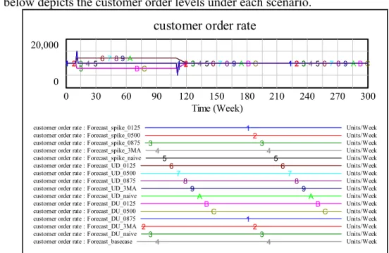
Table 2: Customer order scenarios and the alternate forecast methods Figure 3 below depicts the customer order levels under each scenario.

customer order rate

20,000 0 4 4 4 3 3 3 2 2 2 1 ₁ 1 C C C B B B A A A 9 9 9 8 8 8 7 7 7 6 6 6 5 5 5 4 4 4 3 3 3 2 2 2 1 1 1 0 30 60 90 120 150 180 210 240 270 300 Time (Week)

customer order rate : Forecast_spike_0125 1 Units/Week

customer order rate : Forecast_spike_0500 2 Units/Week

customer order rate : Forecast_spike_0875 3 3 Units/Week

customer order rate : Forecast_spike_3MA 4 4 Units/Week

customer order rate : Forecast_spike_naive 5 5 Units/Week

customer order rate : Forecast_UD_0125 6 6 Units/Week

customer order rate : Forecast_UD_3MA 9 9 Units/Week

customer order rate : Forecast_UD_naive A A Units/Week

customer order rate : Forecast_DU_0125 B B Units/Week

customer order rate : Forecast_DU_0500 C C Units/Week

customer order rate : Forecast_DU_0875 1 Units/Week

customer order rate : Forecast_DU_3MA 2 2 Units/Week

customer order rate : Forecast_DU_naive 3 3 Units/Week

customer order rate : Forecast_basecase 4 4 Units/Week

(7)

Under the base case scenario, there is no change in the steady rate of customer orders and as such the manufacturer’s schedules run like clock work. Under the three alternate scenarios customer orders experience upward, downward movements of different nature, quick jump, quick drop, slow ramp up, a slow ramp down, a one-time spike up, and a one-time spike down. The objective in choosing these varieties is to capture the resultant response behavior of the system under alternate forecast methods to assess the suitability of each forecast method for each type of scenario.

Given that the manufacturer receives orders weekly, one week at a time only, few of the forecast methods would not be suitable for adoption. For example, using a linear regression for such ‘one time unit each step’ would be not practical.

Results from Alternate Policies

Traditional belief has been that the primary objective of a demand forecast is to track the customer orders closely to ensure quick response in production schedules and inventory levels. However, this perception and belief was developed at a time when the supply chain thought had not arrived on the scene and all trading partners were operating, “each in his/her own best interests” oblivious of the schedule changes they were causing to trading partners.

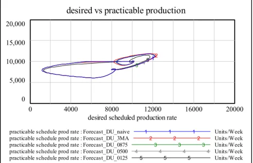
Now, in a changed economic setting of supply chains and mutual cooperation between trading partners, the efficacy of the forecast methods is to be assessed on the basis of least instability in the supply chain operations (read as, least erratic production schedules and inventory levels) rather than a close tracking of customer orders. Figures 4, 5, and 6 below capture the instability in the system under various scenarios.

desired vs practicable production

20,000 15,000 10,000 5,000 0 5 4 3 2 1 0 4000 8000 12000 16000 20000

desired scheduled production rate

practicable schedule prod rate : Forecast_DU_naive 1 1 1 Units/Week

practicable schedule prod rate : Forecast_DU_3MA 2 2 2 Units/Week

practicable schedule prod rate : Forecast_DU_0875 3 3 3 Units/Week

practicable schedule prod rate : Forecast_DU_0500 4 4 4 4 Units/Week

practicable schedule prod rate : Forecast_DU_0125 5 5 5 Units/Week

Figure 4: Phase plot of Desired vs. Practicable production rates in a downward first and then upward change, in customer orders.

(8)

desired vs practicable production3 20,000 16,000 12,000 8,000 4,000 5 ₄ 5 4 4 3 3 3 2 2 2 1 1 4000 8000 12000 16000 20000

practicable schedule prod rate : Forecast_UD_naive 1 1 1 Units/Week

practicable schedule prod rate : Forecast_UD_3MA 2 2 2 Units/Week

practicable schedule prod rate : Forecast_UD_0875 3 3 3 Units/Week

practicable schedule prod rate : Forecast_UD_0500 4 4 4 4 Units/Week

practicable schedule prod rate : Forecast_UD_0125 5 5 5 Units/Week

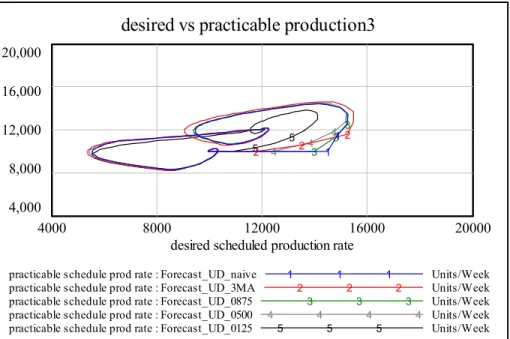
Figure 5: Phase plot of Desired vs. Practicable production rates in a upward first and then downward change, in customer orders.

desired vs practicable production2

20,000 15,000 10,000 5,000 0 5 4 4 3 2 11 0 5000 10000 15000 20000

practicable schedule prod rate : Forecast_spike_naive 1 1 1 Units/Week

practicable schedule prod rate : Forecast_spike_3MA 2 2 2 Units/Week

practicable schedule prod rate : Forecast_spike_0875 3 3 3 Units/Week

Figure 6: Phase plot of Desired vs. Practicable production rates with a one time spike up and one time downward spike, in customer orders. Let us first understand the broad implications of the three scenarios.

Scenario 1: Customer orders first go down by 20% in week 11, and after 100 weeks, at week 111 return to the original level. In other words, customer orders start at 10,000 units/week, go down to 8,000 units/week and revert back to 10,000 units/week.

(9)

Scenario 2: Customer orders first go up by 20% in week 11, and after 100 weeks, at week 111 return to the original level. Here customer orders start at 10,000 units/week, go up to 12,000 units/week and revert back to 10,000 units/week.

Scenario 3: Customer orders experience a (one time) 50% upward spike at week 11 and a (one time) downward spike of 50% at week 111. Here customer orders start at 10,000 units/week, spike to 15,000 units/week at week 11 and continue at 10,000 units/week until week 111, when the orders spike down to 5,000 units/week and continue at 10,000 units/week for the rest.

It is not hard to visualize that the equilibrium point in each of the plots shown in Figures 4, 5, and 6 must lie along the diagonal connecting (0, 0) to (20000, 20000). So effectiveness of each forecasting method is to be assessed by the smooth transition from one equilibrium point (steady state) to the next, with the least amount of disturbance. For example, in Figure 4 the initial equilibrium was at point (10000, 10000) and the second equilibrium point was at (8000, 8000), jumping back to point (10000, 10000) in the later part. In Figure 5, equilibrium moved from (10000, 10000) to (12000, 12000) and reverted back to (10000, 10000) and so on.

While it may not be easily visible but the simple exponential forecasting with a smoothing alpha of 0.125 provides the best result in terms of smooth transition from one equilibrium to the next and back in case of upward trend in customer orders, while forecasting with a smoothing alpha of 0.875 is better when customer orders are on the decline, under each of the three scenarios. A faster convergence to the next steady state means, ease in transition in terms of ease in implementation, better schedules, more stable and reliable order forecasting.

Our intent here is to suggest the need for an analytical assessment of alternate forecast choices given the management policies in respect of inventories and finished goods and WIP replenishment, paving the way for a dynamic forecast policy formulation.

As a matter fact, the result in this study may not come as a surprise result for a system

dynamicist who knows very well that, aggressive corrective action in a negative feedback loop situation results in overshoot and oscillations (Forrester, 1958; Sterman, 2000). The forecasting of next time-period demand is but a negative feedback loop of the form,

(desired state - current state)/time to adjust.

Contributions and Limitations

Anyone driving an automobile knows very well that, when negotiating sharp turns, prudence lies in slowing down to negotiate the turn, or a loss of control is probable (a la, an unintended side effect). Some contributions of this study are: a) highlights the need for manufacturers to understand the effect of forecasting policies on supply chain dynamics, b) demonstrates that a good forecast policy is one that causes minimal disability in supply chain schedules rather than one that tracks the history of customer orders closely, c) reaffirms the usefulness of information visibility in addressing the bullwhip effect, and d) emphasizes that other complementary

strategies can enhance the effectiveness of information visibility policy.

(10)

complex real world. For example, the following explicit assumptions were made to simplify the model. a) uniform shipping cost per unit, b) uniform ordering costs, c) decimal values allowed in the workforce numbers, d) supplier is assumed to be servicing a single manufacturer, and e) sufficient surplus capacities are assumed available at both supplier’s and manufacturer’s facilities.

Interests of the entire supply chain partners are served the best when each partner in the supply chain removes the aggressive corrections that would result in destabilizing the smooth functioning of the supply chain besides sharing the order and scheduling information.

REFERENCES

Akkermans, H., and Dellaert, N. (2005). “Rediscovery of industrial dynamics: contributions of system dynamics to supply chain management in a dynamics and fragmented world,” System Dynamics Review Volume 21, No3, (fall)

Beamon BM.. (1998). Supply chain design and analysis: Models and methods, International Journal of Production Economics, 55, pp 281-294.

Croson, R, and Donohue K, (2005). “Upstream versus downstream information and its impact on bullwhip effect,” System Dynamics Review Volume 21, No 3, (fall)

Croson R, Donohue K, (2003). “The impact of POS data sharing on supply chain management; an experimental study” Production and Operations Management 12: pp1-11.

Forrester, Jay W, (1958). “ Industrial dynamics: a major breakthrough for decision makers,” Harvard Business Review 36(4); 37-66.

Forrester, Jay W, (1961). Industrial Dynamics, MIT Press, Cambridge, MA (now available from Pegasus Communications, Waltham, MA).

Geary S, Disney SM, and Towill DR. (2006). On bullwhip in supply chains – historical review, present practice and expected future impact International Journal of Production Economics, 101, pp 2-18.

Holmstro m J. (1997). Product range management: A case study of supply chain operations in the European grocery industry. International Journal of Supply Chain Management 2 (8), 107– 115.

Lee HL, Padmanabhan V, Whang S. (1997a). Information distortion in a supply chain: the bullwhip effect Management Science, 43 (4), pp 546-548.

Lee HL, Padmanabhan V, Whang S. (1997b). The Bullwhip effect in Supply Chain Sloan Management Review, spring, pp 93-102.

Metters R. (1997). Quantifying the bullwhip effect in supply chains. Journal of Operations Management 15, 89–100.

Sterman, John D., (2000). Business Dynamics-Systems Thinking and Modeling for a Complex World McGrawHill Companies Inc.