arXiv:quant-ph/9508027v2 25 Jan 1996
Peter W. Shor
†Abstract
A digital computer is generally believed to be an efficient universal computing device; that is, it is believed able to simulate any physical computing device with an increase in computation time by at most a polynomial factor. This may not be true when quantum mechanics is taken into consideration. This paper considers factoring integers and finding discrete logarithms, two problems which are generally thought to be hard on a classical computer and which have been used as the basis of several proposed cryptosystems. Efficient randomized algorithms are given for these two problems on a hypothetical quantum computer. These algorithms take a number of steps polynomial in the input size, e.g., the number of digits of the integer to be factored.
Keywords: algorithmic number theory, prime factorization, discrete logarithms, Church’s thesis, quantum computers, foundations of quantum mechanics, spin systems, Fourier transforms
AMS subject classifications: 81P10, 11Y05, 68Q10, 03D10
∗A preliminary version of this paper appeared in the Proceedings of the 35th Annual Symposium
on Foundations of Computer Science, Santa Fe, NM, Nov. 20–22, 1994, IEEE Computer Society Press, pp. 124–134.
†AT&T Research, Room 2D-149, 600 Mountain Ave., Murray Hill, NJ 07974.
1
Introduction
One of the first results in the mathematics of computation, which underlies the subse-quent development of much of theoretical computer science, was the distinction between computable and non-computable functions shown in papers of Church [1936], Turing [1936], and Post [1936]. Central to this result is Church’s thesis, which says that all computing devices can be simulated by a Turing machine. This thesis greatly simpli-fies the study of computation, since it reduces the potential field of study from any of an infinite number of potential computing devices to Turing machines. Church’s thesis is not a mathematical theorem; to make it one would require a precise mathematical description of a computing device. Such a description, however, would leave open the possibility of some practical computing device which did not satisfy this precise math-ematical description, and thus would make the resulting mathmath-ematical theorem weaker than Church’s original thesis.
With the development of practical computers, it has become apparent that the dis-tinction between computable and non-computable functions is much too coarse; com-puter scientists are now interested in the exact efficiency with which specific functions can be computed. This exact efficiency, on the other hand, is too precise a quantity to work with easily. The generally accepted compromise between coarseness and precision distinguishes efficiently and inefficiently computable functions by whether the length of the computation scales polynomially or superpolynomially with the input size. The class of problems which can be solved by algorithms having a number of steps polynomial in the input size is known as P.
For this classification to make sense, we need it to be machine-independent. That is, we need to know that whether a function is computable in polynomial time is indepen-dent of the kind of computing device used. This corresponds to the following quantitative version of Church’s thesis, which Vergis et al. [1986] have called the “Strong Church’s Thesis” and which makes up half of the “Invariance Thesis” of van Emde Boas [1990].
Thesis (Quantitative Church’s thesis). Any physical computing device can be simu-lated by a Turing machine in a number of steps polynomial in the resources used by the computing device.
In statements of this thesis, the Turing machine is sometimes augmented with a ran-dom number generator, as it has not yet been determined whether there are pseudoran-dom number generators which can efficiently simulate truly ranpseudoran-dom number generators for all purposes. Readers who are not comfortable with Turing machines may think instead of digital computers having an amount of memory that grows linearly with the length of the computation, as these two classes of computing machines can efficiently simulate each other.
There are two escape clauses in the above thesis. One of these is the word “physical.” Researchers have produced machine models that violate the above quantitative Church’s thesis, but most of these have been ruled out by some reason for why they are not “phys-ical,” that is, why they could not be built and made to work. The other escape clause in the above thesis is the word “resources,” the meaning of which is not completely speci-fied above. There are generally two resources which limit the ability of digital computers to solve large problems: time (computation steps) and space (memory). There are more resources pertinent to analog computation; some proposed analog machines that seem able to solve NP-complete problems in polynomial time have required the machining of
exponentially precise parts, or an exponential amount of energy. (See Vergis et al. [1986] and Steiglitz [1988]; this issue is also implicit in the papers of Canny and Reif [1987] and Choi et al. [1995] on three-dimensional shortest paths.)
For quantum computation, in addition to space and time, there is also a third poten-tially important resource, precision. For a quantum computer to work, at least in any currently envisioned implementation, it must be able to make changes in the quantum states of objects (e.g., atoms, photons, or nuclear spins). These changes can clearly not be perfectly accurate, but must contain some small amount of inherent impreci-sion. If this imprecision is constant (i.e., it does not depend on the size of the input), then it is not known how to compute any functions in polynomial time on a quantum computer that cannot also be computed in polynomial time on a classical computer with a random number generator. However, if we let the precision grow polynomially in the input size (that is, we let the number of bits of precision grow logarithmically in the input size), we appear to obtain a more powerful type of computer. Allowing the same polynomial growth in precision does not appear to confer extra computing power to classical mechanics, although allowing exponential growth in precision does [Hartmanis and Simon 1974, Vergis et al. 1986].
As far as we know, what precision is possible in quantum state manipulation is dic-tated not by fundamental physical laws but by the properties of the materials and the architecture with which a quantum computer is built. It is currently not clear which architectures, if any, will give high precision, and what this precision will be. If the pre-cision of a quantum computer is large enough to make it more powerful than a classical computer, then in order to understand its potential it is important to think of precision as a resource that can vary. Treating the precision as a large constant (even though it is almost certain to be constant for any given machine) would be comparable to treating a classical digital computer as a finite automaton — since any given computer has a fixed amount of memory, this view is technically correct; however, it is not particularly useful.
Because of the remarkable effectiveness of our mathematical models of computation, computer scientists have tended to forget that computation is dependent on the laws of physics. This can be seen in the statement of the quantitative Church’s thesis in van Emde Boas [1990], where the word “physical” in the above phrasing is replaced with the word “reasonable.” It is difficult to imagine any definition of “reasonable” in this context which does not mean “physically realizable,” i.e., that this computing machine could actually be built and would work.
Computer scientists have become convinced of the truth of the quantitative Church’s thesis through the failure of all proposed counter-examples. Most of these proposed counter-examples have been based on the laws of classical mechanics; however, the uni-verse is in reality quantum mechanical. Quantum mechanical objects often behave quite differently from how our intuition, based on classical mechanics, tells us they should. It thus seems plausible that the natural computing power of classical mechanics corre-sponds to Turing machines,1 while the natural computing power of quantum mechanics
might be greater.
1I believe that this question has not yet been settled and is worthy of further investigation. See
Vergis et al. [1986], Steiglitz [1988], and Rubel [1989]. In particular, turbulence seems a good candidate for a counterexample to the quantitative Church’s thesis because the non-trivial dynamics on many length scales may make it difficult to simulate on a classical computer.
The first person to look at the interaction between computation and quantum me-chanics appears to have been Benioff [1980, 1982a, 1982b]. Although he did not ask whether quantum mechanics conferred extra power to computation, he showed that re-versible unitary evolution was sufficient to realize the computational power of a Turing machine, thus showing that quantum mechanics is at least as powerful computationally as a classical computer. This work was fundamental in making later investigation of quantum computers possible.
Feynman [1982,1986] seems to have been the first to suggest that quantum mechanics might be more powerful computationally than a Turing machine. He gave arguments as to why quantum mechanics might be intrinsically expensive computationally to simulate on a classical computer. He also raised the possibility of using a computer based on quantum mechanical principles to avoid this problem, thus implicitly asking the converse question: by using quantum mechanics in a computer can you compute more efficiently than on a classical computer? Deutsch [1985, 1989] was the first to ask this question explicitly. In order to study this question, he defined both quantum Turing machines and quantum circuits and investigated some of their properties.
The question of whether using quantum mechanics in a computer allows one to obtain more computational power was more recently addressed by Deutsch and Jozsa [1992] and Berthiaume and Brassard [1992a, 1992b]. These papers showed that there are problems which quantum computers can quickly solve exactly, but that classical computers can only solve quickly with high probability and the aid of a random number generator. However, these papers did not show how to solve any problem in quantum polynomial time that was not already known to be solvable in polynomial time with the aid of a random number generator, allowing a small probability of error; this is the characterization of the complexity class BPP, which is widely viewed as the class of efficiently solvable problems.
Further work on this problem was stimulated by Bernstein and Vazirani [1993]. One of the results contained in their paper was an oracle problem (that is, a problem involving a “black box” subroutine that the computer is allowed to perform, but for which no code is accessible) which can be done in polynomial time on a quantum Turing machine but which requires super-polynomial time on a classical computer. This result was improved by Simon [1994], who gave a much simpler construction of an oracle problem which takes polynomial time on a quantum computer but requires exponential time on a classical computer. Indeed, while Bernstein and Vaziarni’s problem appears contrived, Simon’s problem looks quite natural. Simon’s algorithm inspired the work presented in this paper.
Two number theory problems which have been studied extensively but for which no polynomial-time algorithms have yet been discovered are finding discrete logarithms and factoring integers [Pomerance 1987, Gordon 1993, Lenstra and Lenstra 1993, Adleman and McCurley 1995]. These problems are so widely believed to be hard that several cryptosystems based on their difficulty have been proposed, including the widely used RSA public key cryptosystem developed by Rivest, Shamir, and Adleman [1978]. We show that these problems can be solved in polynomial time on a quantum computer with a small probability of error.
Currently, nobody knows how to build a quantum computer, although it seems as though it might be possible within the laws of quantum mechanics. Some suggestions have been made as to possible designs for such computers [Teich et al. 1988, Lloyd 1993,
1994, Cirac and Zoller 1995, DiVincenzo 1995, Sleator and Weinfurter 1995, Barenco et al. 1995b, Chuang and Yamomoto 1995], but there will be substantial difficulty in build-ing any of these [Landauer 1995a, Landauer 1995b, Unruh 1995, Chuang et al. 1995, Palma et al. 1995]. The most difficult obstacles appear to involve the decoherence of quantum superpositions through the interaction of the computer with the environment, and the implementation of quantum state transformations with enough precision to give accurate results after many computation steps. Both of these obstacles become more difficult as the size of the computer grows, so it may turn out to be possible to build small quantum computers, while scaling up to machines large enough to do interesting computations may present fundamental difficulties.
Even if no useful quantum computer is ever built, this research does illuminate the problem of simulating quantum mechanics on a classical computer. Any method of doing this for an arbitrary Hamiltonian would necessarily be able to simulate a quantum computer. Thus, any general method for simulating quantum mechanics with at most a polynomial slowdown would lead to a polynomial-time algorithm for factoring.
The rest of this paper is organized as follows. In §2, we introduce the model of quantum computation, thequantum gate array, that we use in the rest of the paper. In §§3 and 4, we explain two subroutines that are used in our algorithms: reversible modular exponentiation in §3 and quantum Fourier transforms in §4. In §5, we give our algorithm for prime factorization, and in §6, we give our algorithm for extracting discrete logarithms. In §7, we give a brief discussion of the practicality of quantum computation and suggest possible directions for further work.
2
Quantum computation
In this section we give a brief introduction to quantum computation, emphasizing the properties that we will use. We will describe only quantum gate arrays, or quantum acyclic circuits, which are analogous to acyclic circuits in classical computer science. For other models of quantum computers, see references on quantum Turing machines [Deutsch 1989, Bernstein and Vazirani 1993, Yao 1993] and quantum cellular automata [Feynman 1986, Margolus 1986, 1990, Lloyd 1993, Biafore 1994]. If they are allowed a small probability of error, quantum Turing machines and quantum gate arrays can compute the same functions in polynomial time [Yao 1993]. This may also be true for the various models of quantum cellular automata, but it has not yet been proved. This gives evidence that the class of functions computable in quantum polynomial time with a small probability of error is robust, in that it does not depend on the exact architecture of a quantum computer. By analogy with the classical class BPP, this class is called BQP.
Consider a system with ncomponents, each of which can have two states. Whereas in classical physics, a complete description of the state of this system requires onlyn
bits, in quantum physics, a complete description of the state of this system requires 2n −1 complex numbers. To be more precise, the state of the quantum system is a
point in a 2n-dimensional vector space. For each of the 2n possible classical positions
of the components, there is a basis state of this vector space which we represent, for example, by |011· · ·0i meaning that the first bit is 0, the second bit is 1, and so on. Here, theket notation|ximeans thatxis a (pure) quantum state. (Mixed states will
not be discussed in this paper, and thus we do not define them; see a quantum theory book such as Peres [1993] for this definition.) The Hilbert space associated with this quantum system is the complex vector space with these 2n states as basis vectors, and
the state of the system at any time is represented by a unit-length vector in this Hilbert space. As multiplying this state vector by a unit-length complex phase does not change any behavior of the state, we need only 2n−1 complex numbers to completely describe
the state. We represent this superposition of states as
2n −1 X
i=0
ai|Sii, (2.1)
where the amplitudes ai are complex numbers such that Pi|ai|2 = 1 and each |Sii
is a basis vector of the Hilbert space. If the machine is measured (with respect to this basis) at any particular step, the probability of seeing basis state |Sii is |ai|2;
however, measuring the state of the machine projects this state to the observed basis vector|Sii. Thus, looking at the machine during the computation will invalidate the
rest of the computation. In this paper, we only consider measurements with respect to the canonical basis. This does not greatly restrict our model of computation, since measurements in other reasonable bases could be simulated by first using quantum computation to perform a change of basis and then performing a measurement in the canonical basis.
In order to use a physical system for computation, we must be able to change the state of the system. The laws of quantum mechanics permit only unitary transforma-tions of state vectors. A unitary matrix is one whose conjugate transpose is equal to its inverse, and requiring state transformations to be represented by unitary matrices ensures that summing the probabilities of obtaining every possible outcome will result in 1. The definition of quantum circuits (and quantum Turing machines) only allows
local unitary transformations; that is, unitary transformations on a fixed number of bits. This is physically justified because, given a general unitary transformation onn
bits, it is not at all clear how one would efficiently implement it physically, whereas two-bit transformations can at least in theory be implemented by relatively simple physical systems [Cirac and Zoller 1995, DiVincenzo 1995, Sleator and Weinfurter 1995, Chuang and Yamomoto 1995]. While general n-bit transformations can always be built out of two-bit transformations [DiVincenzo 1995, Sleator and Weinfurter 1995, Lloyd 1995, Deutsch et al. 1995], the number required will often be exponential in n
[Barenco et al. 1995a]. Thus, the set of two-bit transformations form a set of building blocks for quantum circuits in a manner analogous to the way a universal set of classical gates (such as the AND, OR and NOT gates) form a set of building blocks for classical circuits. In fact, for a universal set of quantum gates, it is sufficient to take all one-bit gates and a single type of two-bit gate, the controlled NOT, which negates the second bit if and only if the first bit is 1.
Perhaps an example will be informative at this point. A quantum gate can be expressed as a truth table: for each input basis vector we need to give the output of the gate. One such gate is:
|00i → |00i |01i → |01i (2.2) |10i → √1 2(|10i+|11i) |11i → √1 2(|10i − |11i).
Not all truth tables correspond to physically feasible quantum gates, as many truth tables will not give rise to unitary transformations.
The same gate can also be represented as a matrix. The rows correspond to input basis vectors. The columns correspond to output basis vectors. The (i, j) entry gives, when theith basis vector is input to the gate, the coefficient of thejth basis vector in the corresponding output of the gate. The truth table above would then correspond to the following matrix:
|00i |01i |10i |11i |00i 1 0 0 0 |01i 0 1 0 0 |10i 0 0 √1 2 1 √ 2 |11i 0 0 √1 2 − 1 √ 2 . (2.3)
A quantum gate is feasible if and only if the corresponding matrix is unitary, i.e., its inverse is its conjugate transpose.
Suppose our machine is in the superposition of states
1 √ 2|10i − 1 √ 2|11i (2.4)
and we apply the unitary transformation represented by (2.2) and (2.3) to this state. The resulting output will be the result of multiplying the vector (2.4) by the matrix (2.3). The machine will thus go to the superposition of states
1
2(|10i+|11i)− 1
2(|10i − |11i) = |11i. (2.5)
This example shows the potential effects of interference on quantum computation. Had we started with either the state|10ior the state|11i, there would have been a chance of observing the state|10iafter the application of the gate (2.3). However, when we start with a superposition of these two states, the probability amplitudes for the state|10i
cancel, and we have no possibility of observing |10i after the application of the gate. Notice that the output of the gate would have been|10iinstead of|11ihad we started with the superposition of states
1 √ 2|10i+ 1 √ 2|11i (2.6)
which has the same probabilities of being in any particular configuration if it is observed as does the superposition (2.4).
If we apply a gate to only two bits of a longer basis vector (now our circuit must have more than two wires), we multiply the gate matrix by the two bits to which the gate is
applied, and leave the other bits alone. This corresponds to multiplying the whole state by the tensor product of the gate matrix on those two bits with the identity matrix on the remaining bits.
A quantum gate array is a set of quantum gates with logical “wires” connecting their inputs and outputs. The input to the gate array, possibly along with extra work bits that are initially set to 0, is fed through a sequence of quantum gates. The values of the bits are observed after the last quantum gate, and these values are the output. To compare gate arrays with quantum Turing machines, we need to add conditions that make gate arrays auniformcomplexity class. In other words, because there is a different gate array for each size of input, we need to keep the designer of the gate arrays from hiding non-computable (or hard to compute) information in the arrangement of the gates. To make quantum gate arrays uniform, we must add two things to the definition of gate arrays. The first is the standard requirement that the design of the gate array be produced by a polynomial-time (classical) computation. The second requirement should be a standard part of the definition of analog complexity classes, although since analog complexity classes have not been widely studied, this requirement is much less widely known. This requirement is that the entries in the unitary matrices describing the gates must be computable numbers. Specifically, the first lognbits of each entry should be classically computable in time polynomial in n [Solovay 1995]. This keeps non-computable (or hard to compute) information from being hidden in the bits of the amplitudes of the quantum gates.
3
Reversible logic and modular exponentiation
The definition of quantum gate arrays gives rise to completely reversible computation. That is, knowing the quantum state on the wires leading out of a gate tells uniquely what the quantum state must have been on the wires leading into that gate. This is a reflection of the fact that, despite the macroscopic arrow of time, the laws of physics ap-pear to be completely reversible. This would seem to imply that anything built with the laws of physics must be completely reversible; however, classical computers get around this fact by dissipating energy and thus making their computations thermodynamically irreversible. This appears impossible to do for quantum computers because superpo-sitions of quantum states need to be maintained throughout the computation. Thus, quantum computers necessarily have to use reversible computation. This imposes ex-tra costs when doing classical computations on a quantum computer, as is sometimes necessary in subroutines of quantum computations.
Because of the reversibility of quantum computation, a deterministic computation is performable on a quantum computer only if it is reversible. Luckily, it has already been shown that any deterministic computation can be made reversible [Lecerf 1963, Bennett 1973]. In fact, reversible classical gate arrays have been studied. Much like the result that any classical computation can be done using NAND gates, there are also universal gates for reversible computation. Two of these are Toffoli gates [Toffoli 1980] and Fredkin gates [Fredkin and Toffoli 1982]; these are illustrated in Table 3.1.
The Toffoli gate is just a controlled controlled NOT, i.e., the last bit is negated if and only if the first two bits are 1. In a Toffoli gate, if the third input bit is set to 1, then the third output bit is the NAND of the first two input bits. Since NAND is a
Table 3.1: Truth tables for Toffoli and Fredkin gates. Toffoli Gate INPUT OUTPUT 0 0 0 0 0 0 0 0 1 0 0 1 0 1 0 0 1 0 0 1 1 0 1 1 1 0 0 1 0 0 1 0 1 1 0 1 1 1 0 1 1 1 1 1 1 1 1 0 Fredkin Gate INPUT OUTPUT 0 0 0 0 0 0 0 0 1 0 1 0 0 1 0 0 0 1 0 1 1 0 1 1 1 0 0 1 0 0 1 0 1 1 0 1 1 1 0 1 1 0 1 1 1 1 1 1
universal gate for classical gate arrays, this shows that the Toffoli gate is universal. In a Fredkin gate, the last two bits are swapped if the first bit is 0, and left untouched if the first bit is 1. For a Fredkin gate, if the third input bit is set to 0, the second output bit is the AND of the first two input bits; and if the last two input bits are set to 0 and 1 respectively, the second output bit is the NOT of the first input bit. Thus, both AND and NOT gates are realizable using Fredkin gates, showing that the Fredkin gate is universal.
From results on reversible computation [Lecerf 1963, Bennett 1973], we can compute any polynomial time functionF(x) as long as we keep the inputxin the computer. We do this by adapting the method for computing the functionF non-reversibly. These results can easily be extended to work for gate arrays [Toffoli 1980, Fredkin and Toffoli 1982]. When AND, OR or NOT gates are changed to Fredkin or Toffoli gates, one obtains both additional input bits, which must be preset to specified values, and additional output bits, which contain the information needed to reverse the computation. While the additional input bits do not present difficulties in designing quantum computers, the additional output bits do, because unless they are all reset to 0, they will affect the interference patterns in quantum computation. Bennett’s method for resetting these bits to 0 is shown in the top half of Table 3.2. A non-reversible gate array may thus be turned into a reversible gate array as follows. First, duplicate the input bits as many times as necessary (since each input bit could be used more than once by the gate array). Next, keeping one copy of the input around, use Toffoli and Fredkin gates to simulate non-reversible gates, putting the extra output bits into the RECORD register. These extra output bits preserve enough of a record of the operations to enable the computation of the gate array to be reversed. Once the outputF(x) has been computed, copy it into a register that has been preset to zero, and then undo the computation to erase both the first OUTPUT register and the RECORD register.
To erasexand replace it withF(x), in addition to a polynomial-time algorithm forF, we also need a polynomial-time algorithm for computingxfromF(x); i.e., we need that
Fis one-to-one and that bothFandF−1are polynomial-time computable. The method
for this computation is given in the whole of Table 3.2. There are two stages to this computation. The first is the same as before, taking x to (x, F(x)). For the second stage, shown in the bottom half of Table 3.2, note that if we have a method to compute
F−1non-reversibly in polynomial time, we can use the same technique to reversibly map
Table 3.2: Bennett’s method for making a computation reversible. INPUT - - -
-INPUT OUTPUT RECORD(F)
-INPUT OUTPUT RECORD(F) OUTPUT
INPUT - - - OUTPUT
INPUT INPUT RECORD(F−1) OUTPUT
- - - INPUT RECORD(F−1) OUTPUT
- - - OUTPUT
we can reverse it to go from (x, F(x)) toF(x). Put together, these two pieces takexto
F(x).
The above discussion shows that computations can be made reversible for only a constant factor cost in time, but the above method uses as much space as it does time. If the classical computation requires much less space than time, then making it reversible in this manner will result in a large increase in the space required. There are methods that do not use as much space, but use more time, to make computations reversible [Bennett 1989, Levine and Sherman 1990]. While there is no general method that does not cause an increase in either space or time, specific algorithms can sometimes be made reversible without paying a large penalty in either space or time; at the end of this section we will show how to do this for modular exponentiation, which is a subroutine necessary for quantum factoring.
The bottleneck in the quantum factoring algorithm; i.e., the piece of the fac-toring algorithm that consumes the most time and space, is modular exponentia-tion. The modular exponentiation problem is, given n, x, and r, find xr (modn).
The best classical method for doing this is to repeatedly square of x(mod n) to get x2i
(mod n) for i ≤ log2r, and then multiply a subset of these powers (modn)
to get xr (modn). If we are working with l-bit numbers, this requires O(l)
squar-ings and multiplications of l-bit numbers (modn). Asymptotically, the best clas-sical result for gate arrays for multiplication is the Sch¨onhage–Strassen algorithm [Sch¨onhage and Strassen 1971, Knuth 1981, Sch¨onhage 1982]. This gives a gate array for integer multiplication that usesO(llogllog logl) gates to multiply twol-bit numbers. Thus, asymptotically, modular exponentiation requiresO(l2logllog logl) time. Making
this reversible would na¨ıvely cost the same amount in space; however, one can reuse the space used in the repeated squaring part of the algorithm, and thus reduce the amount of space needed to essentially that required for multiplying twol-bit numbers; one simple method for reducing this space (although not the most versatile one) will be given later in this section. Thus, modular exponentiation can be done inO(l2logllog logl) time
andO(llogllog logl) space.
While the Sch¨onhage–Strassen algorithm is the best multiplication algorithm discov-ered to date for largel, it does not scale well for small l. For small numbers, the best gate arrays for multiplication essentially use elementary-school longhand multiplication in binary. This method requires O(l2) time to multiply two l-bit numbers, and thus
modular exponentiation requires O(l3) time with this method. These gate arrays can
be made reversible, however, using onlyO(l) space.
O(l) space and O(l ) time to compute (a, x (modn)) from a, wherea, x, andn are
l-bit numbers. The basic building block used is a gate array that takesb as input and outputsb+c (modn). Note that hereb is the gate array’s input butcand nare built into the structure of the gate array. Since addition (modn) is computable inO(logn) time classically, this reversible gate array can be made with only O(logn) gates and
O(logn) work bits using the techniques explained earlier in this section.
The technique we use for computingxa (modn) is essentially the same as the
classi-cal method. First, by repeated squaring we computex2i
(modn) for alli < l. Then, to obtainxa (modn) we multiply the powers x2i
(modn) where 2i appears in the binary
expansion ofa. In our algorithm for factoringn, we only need to computexa (modn)
wherea is in a superposition of states, but xis some fixed integer. This makes things much easier, because we can use a reversible gate array where a is treated as input, but wherexandnare built into the structure of the gate array. Thus, we can use the algorithm described by the following pseudocode; here,ai represents theith bit ofain
binary, where the bits are indexed from right to left and the rightmost bit ofaisa0.
power := 1 for i = 0 to l−1 if ( ai == 1 ) then power := power ∗ x2i (mod n) endif endfor
The variableais left unchanged by the code andxa (mod n) is output as the variable
power. Thus, this code takes the pair of values (a,1) to (a, xa (modn)).
This pseudocode can easily be turned into a gate array; the only hard part of this is the fourth line, where we multiply the variablepower byx2i (modn); to do this we
need to use a fairly complicated gate array as a subroutine. Recall that x2i (modn)
can be computed classically and then built into the structure of the gate array. Thus, to implement this line, we need a reversible gate array that takesb as input and gives
bc(modn) as output, where the structure of the gate array can depend on c and n. Of course, this step can only be reversible if gcd(c, n) = 1, i.e., if c and n have no common factors, as otherwise two distinct values ofbwill be mapped to the same value ofbc(modn); this case is fortunately all we need for the factoring algorithm. We will show how to build this gate array in two stages. The first stage is directly analogous to exponentiation by repeated multiplication; we obtain multiplication from repeated addition (modn). Pseudocode for this stage is as follows.
result := 0
for i = 0 to l−1
if ( bi == 1 ) then
result := result + 2ic (mod n)
endif endfor
The above pseudocode takes b as input, and gives (b, bc(mod n)) as output. To get the desired result, we now need to eraseb. Recall that gcd(c, n) = 1, so there is a c−1 (modn) with c c−1 ≡ 1 (modn). Multiplication by this c−1 could be used to
reversibly take bc(modn) to (bc(modn), bcc−1(mod n)) = (bc(modn), b). This is
just the reverse of the operation we want, and since we are working with reversible computing, we can turn this operation around to erase b. The pseudocode for this follows. for i = 0 to l−1 if ( resulti == 1 ) then b := b − 2ic−1 (modn) endif endfor
As before,resulti is theith bit ofresult.
Note that at this stage of the computation,bshould be 0. However, we did not setb
directly to zero, as this would not have been a reversible operation and thus impossible on a quantum computer, but instead we did a relatively complicated sequence of operations which ended with b = 0 and which in fact depended on multiplication being a group (modn). At this point, then, we could do something somewhat sneaky: we could measure b to see if it actually is 0. If it is not, we know that there has been an error somewhere in the quantum computation, i.e., that the results are worthless and we should stop the computer and start over again. However, if we do find that b is 0, then we know (because we just observed it) that it is now exactly 0. This measurement thus may bring the quantum computation back on track in that any amplitude thatb
had for being non-zero has been eliminated. Further, because the probability that we observe a state is proportional to the square of the amplitude of that state, depending on the error model, doing the modular exponentiation and measuringb every time that we know that it should be 0 may have a higher probability of overall success than the same computation done without the repeated measurements ofb; this is the quantum watchdog(orquantum Zeno) effect [Peres 1993]. The argument above does not actually show that repeated measurement ofbis indeed beneficial, because there is a cost (in time, if nothing else) of measuringb. Before this is implemented, then, it should be checked with analysis or experiment that the benefit of such measurements exceeds their cost. However, I believe that partial measurements such as this one are a promising way of trying to stabilize quantum computations.
Currently, Sch¨onhage–Strassen is the algorithm of choice for multiplying very large numbers, and longhand multiplication is the algorithm of choice for small numbers. There are also multiplication algorithms which have efficiencies between these two al-gorithms, and which are the best algorithms to use for intermediate length numbers [Karatsuba and Ofman 1962, Knuth 1981, Sch¨onhage et al. 1994]. It is not clear which algorithms are best for which size numbers. While this may be known to some extent for classical computation [Sch¨onhage et al. 1994], using data on which algorithms work better on classical computers could be misleading for two reasons: First, classical com-puters need not be reversible, and the cost of making an algorithm reversible depends on the algorithm. Second, existing computers generally have multiplication for 32- or 64-bit numbers built into their hardware, and this will increase the optimal changeover
points to asymptotically faster algorithms; further, some multiplication algorithms can take better advantage of this hardwired multiplication than others. Thus, in order to program quantum computers most efficiently, work needs to be done on the best way of implementing elementary arithmetic operations on quantum computers. One tantalizing fact is that the Sch¨onhage–Strassen fast multiplication algorithm uses the fast Fourier transform, which is also the basis for all the fast algorithms on quantum computers discovered to date; it is tempting to speculate that integer multiplication itself might be speeded up by a quantum algorithm; if possible, this would result in a somewhat faster asymptotic bound for factoring on a quantum computer, and indeed could even make breaking RSA on a quantum computer asymptotically faster than encrypting with RSA on a classical computer.
4
Quantum Fourier transforms
Since quantum computation deals with unitary transformations, it is helpful to be able to build certain useful unitary transformations. In this section we give a technique for constructing in polynomial time on quantum computers one particular unitary transfor-mation, which is essentially a discrete Fourier transform. This transformation will be given as a matrix, with both rows and columns indexed by states. These states corre-spond to binary representations of integers on the computer; in particular, the rows and columns will be indexed beginning with 0 unless otherwise specified.
This transformations is as follows. Consider a numbera with 0≤a < q for someq
where the number of bits ofq is polynomial. We will perform the transformation that takes the state|aito the state
1 q1/2 q−1 X c=0 |ciexp(2πiac/q). (4.1)
That is, we apply the unitary matrix whose (a, c) entry isq11/2exp(2πiac/q). This Fourier transform is at the heart of our algorithms, and we call this matrixAq.
Since we will useAq forqof exponential size, we must show how this transformation
can be done in polynomial time. In this paper, we will give a simple construction forAq
whenq is a power of 2 that was discovered independently by Coppersmith [1994] and Deutsch [see Ekert and Jozsa 1995]. This construction is essentially the standard fast Fourier transform (FFT) algorithm [Knuth 1981] adapted for a quantum computer; the following description of it follows that of Ekert and Jozsa [1995]. In the earlier version of this paper [Shor 1994], we gave a construction forAq whenqwas in the special class
of smooth numbers with small prime power factors. In fact, Cleve [1994] has shown how to constructAq for all smooth numbersqwhose prime factors are at mostO(logn).
Takeq= 2l, and let us represent an integerain binary as|a
l−1al−2. . . a0i. For the
quantum Fourier transformAq, we only need to use two types of quantum gates. These
gates areRj, which operates on thejth bit of the quantum computer:
Rj = |0i |1i |0i √1 2 1 √ 2 |1i √1 2 − 1 √ 2 , (4.2)
andSj,k, which operates on the bits in positionsj andkwithj < k: Sj,k = |00i |01i |10i |11i |00i 1 0 0 0 |01i 0 1 0 0 |10i 0 0 1 0 |11i 0 0 0 eiθk−j , (4.3)
whereθk−j =π/2k−j. To perform a quantum Fourier transform, we apply the matrices
in the order (from left to right)
Rl−1Sl−2,l−1Rl−2Sl−3,l−1Sl−3,l−2Rl−3. . . R1S0,l−1S0,l−2. . . S0,2S0,1R0; (4.4)
that is, we apply the gatesRj in reverse order fromRl−1toR0, and betweenRj+1 and
Rj we apply all the gatesSj,k wherek > j. For example, on 3 bits, the matrices would
be applied in the orderR2S1,2R1S0,2S0,1R0. To take the Fourier transform Aq when
q= 2l, we thus need to usel(l−1)/2 quantum gates.
Applying this sequence of transformations will result in a quantum state
1
q1/2 P
bexp(2πiac/q)|bi, where b is the bit-reversal of c, i.e., the binary number
ob-tained by reading the bits ofc from right to left. Thus, to obtain the actual quantum Fourier transform, we need either to do further computation to reverse the bits of |bi
to obtain |ci, or to leave these bits in place and read them in reverse order; either alternative is easy to implement.
To show that this operation actually performs a quantum Fourier transform, consider the amplitude of going from|ai =|al−1. . . a0i to |bi =|bl−1. . . b0i. First, the factors
of 1/√2 in theR matrices multiply to produce a factor of 1/q1/2 overall; thus we need
only worry about the exp(2πiac/q) phase factor in the expression (4.1). The matrices
Sj,kdo not change the values of any bits, but merely change their phases. There is thus
only one way to switch thejth bit fromaj tobj, and that is to use the appropriate entry
in the matrixRj. This entry addsπ to the phase if the bits aj andbj are both 1, and
leaves it unchanged otherwise. Further, the matrixSj,kaddsπ/2k−j to the phase ifaj
andbk are both 1 and leaves it unchanged otherwise. Thus, the phase on the path from
|aito |biis X 0≤j<l πajbj+ X 0≤j<k<l π 2k−jajbk. (4.5)
This expression can be rewritten as
X
0≤j≤k<l
π
2k−jajbk. (4.6)
Sincecis the bit-reversal ofb, this expression can be further rewritten as
X
0≤j≤k<l
π
2k−jajcl−1−k. (4.7)
Making the substitutionl−k−1 fork in this sum, we get
X
0≤j+k<l
2π2
j2k
Now, since adding multiples of 2πdo not affect the phase, we obtain the same phase if we sum over allj andkless than l, obtaining
l−1 X j,k=0 2π2 j2k 2l ajck= 2π 2l l−1 X j=0 2jaj l−1 X k=0 2kck, (4.9)
where the last equality follows from the distributive law of multiplication. Now,q= 2l,
a=Pl−1
j=02
ja
j, and similarly forc, so the above expression is equal to 2πac/q, which is
the phase for the amplitude of|ai → |ciin the transformation (4.1).
When k−j is large in the gate Sj,k in (4.3), we are multiplying by a very small
phase factor. This would be very difficult to do accurately physically, and thus it would be somewhat disturbing if this were necessary for quantum computation. Luckily, Cop-persmith [1994] has shown that one can define an approximate Fourier transform that ignores these tiny phase factors, but which approximates the Fourier transform closely enough that it can also be used for factoring. In fact, this technique reduces the number of quantum gates needed for the (approximate) Fourier transform considerably, as it leaves out most of the gatesSj,k.
5
Prime factorization
It has been known since before Euclid that every integer n is uniquely decomposable into a product of primes. Mathematicians have been interested in the question of how to factor a number into this product of primes for nearly as long. It was only in the 1970’s, however, that researchers applied the paradigms of theoretical computer science to number theory, and looked at the asymptotic running times of factoring algorithms [Adleman 1994]. This has resulted in a great improvement in the efficiency of factoring algorithms. The best factoring algorithm asymptotically is currently the number field sieve [Lenstra et al. 1990, Lenstra and Lenstra 1993], which in order to factor an inte-gerntakes asymptotic running time exp(c(logn)1/3(log logn)2/3) for some constantc.
Since the input, n, is only logn bits in length, this algorithm is an exponential-time algorithm. Our quantum factoring algorithm takes asymptoticallyO((logn)2(log logn) (log log logn)) steps on a quantum computer, along with a polynomial (in logn) amount of post-processing time on a classical computer that is used to convert the output of the quantum computer to factors ofn. While this post-processing could in principle be done on a quantum computer, there is no reason not to use a classical computer if they are more efficient in practice.
Instead of giving a quantum computer algorithm for factoringndirectly, we give a quantum computer algorithm for finding the order of an elementxin the multiplicative group (modn); that is, the least integerr such thatxr≡1 (modn). It is known that
using randomization, factorization can be reduced to finding the order of an element [Miller 1976]; we now briefly give this reduction.
To find a factor of an odd number n, given a method for computing the order r
ofx, choose a randomx(modn), find its orderr, and compute gcd(xr/2−1, n). Here,
gcd(a, b) is the greatest common divisor ofaandb, i.e., the largest integer that divides bothaandb. The Euclidean algorithm [Knuth 1981] can be used to compute gcd(a, b) in polynomial time. Since (xr/2−1)(xr/2+ 1) =xr−1≡0 (modn), the gcd(xr/2−1, n)
fails to be a non-trivial divisor ofnonly ifris odd or ifxr/2≡ −1 (modn). Using this
criterion, it can be shown that this procedure, when applied to a randomx(modn), yields a factor ofnwith probability at least 1−1/2k−1, wherekis the number of distinct
odd prime factors ofn. A brief sketch of the proof of this result follows. Suppose that
n=Qk
i=1p
ai
i . Letri be the order ofx(mod paii). Thenris the least common multiple
of all theri. Consider the largest power of 2 dividing eachri. The algorithm only fails
if all of these powers of 2 agree: if they are all 1, thenris odd andr/2 does not exist; if they are all equal and larger than 1, thenxr/2≡ −1 (modn) sincexr/2≡ −1 (modpαi
i )
for everyi. By the Chinese remainder theorem [Knuth 1981, Hardy and Wright 1979, Theorem 121], choosing anx(modn) at random is the same as choosing for each i a number xi (mod paii) at random, where p
ai
i is the ith prime power factor of n. The
multiplicative group (modpα) for any odd prime powerpαis cyclic [Knuth 1981], so for
any odd prime powerpai
i , the probability is at most 1/2 of choosing anxi having any
particular power of two as the largest divisor of its orderri. Thus each of these powers
of 2 has at most a 50% probability of agreeing with the previous ones, so allk of them agree with probability at most 1/2k−1, and there is at least a 1−1/2k−1 chance that
thexwe choose is good. This scheme will thus work as long asnis odd and not a prime power; finding factors of prime powers can be done efficiently with classical methods.
We now describe the algorithm for finding the order of x(modn) on a quantum computer. This algorithm will use two quantum registers which hold integers represented in binary. There will also be some amount of workspace. This workspace gets reset to 0 after each subroutine of our algorithm, so we will not include it when we write down the state of our machine.
Givenxandn, to find the order ofx, i.e., the leastrsuch thatxr≡1 (modn), we
do the following. First, we findq, the power of 2 withn2≤q <2n2. We will not include
n,x, orqwhen we write down the state of our machine, because we never change these values. In a quantum gate array we need not even keep these values in memory, as they can be built into the structure of the gate array.
Next, we put the first register in the uniform superposition of states representing numbersa(modq). This leaves our machine in state
1 q1/2 q−1 X a=0 |ai |0i. (5.1)
This step is relatively easy, since all it entails is putting each bit in the first register into the superposition √1
2(|0i+|1i).
Next, we compute xa (mod n) in the second register as described in §3. Since we
keepa in the first register this can be done reversibly. This leaves our machine in the state 1 q1/2 q−1 X a=0 |ai |xa (modn)i. (5.2)
We then perform our Fourier transformAq on the first register, as described in §4,
mapping|aito 1 q1/2 q−1 X c=0 exp(2πiac/q)|ci. (5.3)
That is, we apply the unitary matrix with the (a, c) entry equal to q1/2exp(2πiac/q). This leaves our machine in state
1 q q−1 X a=0 q−1 X c=0
exp(2πiac/q)|ci |xa (modn)i. (5.4)
Finally, we observe the machine. It would be sufficient to observe solely the value of |ci in the first register, but for clarity we will assume that we observe both|ciand
|xa (modn)i. We now compute the probability that our machine ends in a particular
state
c, xk (modn)
, where we may assume 0≤k < r. Summing over all possible ways to reach the state
c, xk (modn)
, we find that this probability is
1 q X a:xa≡xk exp(2πiac/q) 2 . (5.5)
where the sum is over alla, 0≤a < q, such thatxa ≡xk (modn). Because the order
ofx isr, this sum is over all a satisfyinga≡k(mod r). Writinga=br+k, we find that the above probability is
1 q ⌊(q−k−1)/r⌋ X b=0 exp(2πi(br+k)c/q) 2 . (5.6)
We can ignore the term of exp(2πikc/q), as it can be factored out of the sum and has magnitude 1. We can also replacerc with {rc}q, where{rc}q is the residue which is
congruent torc (modq) and is in the range−q/2<{rc}q ≤q/2. This leaves us with
the expression 1 q ⌊(q−k−1)/r⌋ X b=0 exp(2πib{rc}q/q) 2 . (5.7)
We will now show that if{rc}q is small enough, all the amplitudes in this sum will be
in nearly the same direction (i.e., have close to the same phase), and thus make the sum large. Turning the sum into an integral, we obtain
1 q Z ⌊q −k−1 r ⌋ 0 exp(2πib{rc}q/q)db+O ⌊(q−k−1)/r⌋ q (exp(2πi{rc}q/q)−1) . (5.8)
If|{rc}q| ≤r/2, the error term in the above expression is easily seen to be bounded by
O(1/q). We now show that if|{rc}q| ≤r/2, the above integral is large, so the probability
of obtaining a statec, xk (mod n)
is large. Note that this condition depends only on
cand is independent ofk. Substituting u=rb/qin the above integral, we get 1 r Z rq⌊ q−k−1 r ⌋ 0 exp2πi{rc}q r u du. (5.9)
Sincek < r, approximating the upper limit of integration by 1 results in only aO(1/q) error in the above expression. If we do this, we obtain the integral
1 r Z 1 0 exp2πi{rc}q r u du. (5.10)
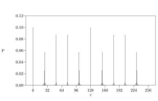
0.00 0.02 0.04 0.06 0.08 0.10 0.12 0 32 64 96 128 160 192 224 256 P c
Figure 5.1: The probability P of observing values ofcbetween 0 and 255, givenq= 256 andr= 10.
Letting{rc}q/r vary between −12 and 1
2, the absolute magnitude of the integral (5.10)
is easily seen to be minimized when {rc}q/r = ±12, in which case the absolute value
of expression (5.10) is 2/(πr). The square of this quantity is a lower bound on the probability that we see any particular state
c, xk (modn)
with {rc}q ≤ r/2; this
probability is thus asymptotically bounded below by 4/(π2r2), and so is at least 1/3r2
for sufficiently largen.
The probability of seeing a given statec, xk (mod n)
will thus be at least 1/3r2if
−r
2 ≤ {rc}q ≤
r
2, (5.11)
i.e., if there is adsuch that
−r
2 ≤rc−dq≤
r
2. (5.12)
Dividing byrqand rearranging the terms gives
c q− d r ≤ 1 2q. (5.13)
We know c andq. Becauseq > n2, there is at most one fraction d/r with r < n that
satisfies the above inequality. Thus, we can obtain the fractiond/r in lowest terms by roundingc/qto the nearest fraction having a denominator smaller thann. This fraction can be found in polynomial time by using a continued fraction expansion ofc/q, which
finds all the best approximations ofc/qby fractions [Hardy and Wright 1979, Chapter X, Knuth 1981].
The exact probabilities as given by equation (5.7) for an example case with r= 10 andq= 256 are plotted in Figure 5.1. The value r= 10 could occur when factoring 33 ifxwere chosen to be 5, for example. Hereqis taken smaller than 332so as to make the
values ofc in the plot distinguishable; this does not change the functional structure of P(c). Note that with high probability the observed value ofcis near an integral multiple ofq/r= 256/10.
If we have the fractiond/rin lowest terms, and if dhappens to be relatively prime tor, this will give usr. We will now count the number of states
c, xk (mod n)
which enable us to computerin this way. There areφ(r) possible values ofdrelatively prime to r, where φ is Euler’s totient function [Knuth 1981, Hardy and Wright 1979, §5.5]. Each of these fractionsd/r is close to one fractionc/q with |c/q−d/r| ≤1/2q. There are alsor possible values forxk, since ris the order ofx. Thus, there arerφ(r) states
c, xk (modn)
which would enable us to obtain r. Since each of these states occurs with probability at least 1/3r2, we obtain r with probability at least φ(r)/3r. Using
the theorem that φ(r)/r > δ/log logr for some constant δ [Hardy and Wright 1979, Theorem 328], this shows that we findrat least aδ/log logrfraction of the time, so by repeating this experiment onlyO(log logr) times, we are assured of a high probability of success.
In practice, assuming that quantum computation is more expensive than classical computation, it would be worthwhile to alter the above algorithm so as to perform less quantum computation and more postprocessing. First, if the observed state is |ci, it would be wise to also try numbers close toc such as c±1, c±2, . . ., since these also have a reasonable chance of being close to a fraction qd/r. Second, if c/q ≈d/r, and
dand r have a common factor, it is likely to be small. Thus, if the observed value of
c/q is rounded off to d′/r′ in lowest terms, for a candidate r one should consider not
onlyr′ but also its small multiples 2r′, 3r′, . . . , to see if these are the actual order ofx. Although the first technique will only reduce the expected number of trials required to find r by a constant factor, the second technique will reduce the expected number of trials for the hardestnfromO(log logn) toO(1) if the first (logn)1+ǫmultiples ofr′are
considered [Odylzko 1995]. A third technique is, if two candidater’s have been found, sayr1andr2, to test the least common multiple ofr1andr2as a candidater. This third
technique is also able to reduce the expected number of trials to a constant [Knill 1995], and will also work in some cases where the first two techniques fail.
Note that in this algorithm for determining the order of an element, we did not use many of the properties of multiplication (modn). In fact, if we have a permutation
f mapping the set {0,1,2, . . . , n−1} into itself such that its kth iterate, f(k)(a), is
computable in time polynomial in logn and logk, the same algorithm will be able to find the order of an elementaunder f, i.e., the minimumrsuch thatf(r)(a) =a.
6
Discrete logarithms
For every primep, the multiplicative group (modp) is cyclic, that is, there are generators
g such that 1, g, g2, . . . , gp−2 comprise all the non-zero residues (mod p) [Hardy and
a generator g. The discrete logarithm of a number x with respect to p and g is the integerrwith 0≤r < p−1 such thatgr≡x(modp). The fastest algorithm known for
finding discrete logarithms modulo arbitrary primespis Gordon’s [1993] adaptation of the number field sieve, which runs in time exp(O(logp)1/3(log logp)2/3)). We show how
to find discrete logarithms on a quantum computer with two modular exponentiations and two quantum Fourier transforms.
This algorithm will use three quantum registers. We first findq a power of 2 such that q is close to p, i.e., with p < q <2p. Next, we put the first two registers in our quantum computer in the uniform superposition of all |ai and |bi (mod p−1), and computegax−b (modp) in the third register. This leaves our machine in the state
1 p−1 p−2 X a=0 p−2 X b=0 a, b, gax−b (mod p) . (6.1)
As before, we use the Fourier transform Aq to send |ai → |ci and |bi → |di with
probability amplitude 1qexp(2πi(ac+bd)/q). This is, we take the state|a, bito the state 1 q q−1 X c=0 q−1 X d=0 exp 2πiq (ac+bd) |c, di. (6.2)
This leaves our quantum computer in the state 1 (p−1)q p−2 X a,b=0 q−1 X c,d=0 exp 2πi q (ac+bd) c, d, gax−b(mod p) . (6.3)
Finally, we observe the state of the quantum computer.
The probability of observing a state|c, d, yiwithy ≡gk (mod p) is
1 (p−1)q X a,b a−rb≡k exp2qπi(ac+bd) 2 (6.4)
where the sum is over all (a, b) such that a−rb ≡k (modp−1). Note that we now have two moduli to deal with, p−1 and q. While this makes keeping track of things more confusing, it does not pose serious problems. We now use the relation
a=br+k−(p−1)jbr+k p−1 k
(6.5) and substitute (6.5) in the expression (6.4) to obtain the amplitude on
c, d, gk (mod p) , which is 1 (p−1)q p−2 X b=0 exp2πi q brc+kc+bd−c(p−1) j br+k p−1 k . (6.6)
The absolute value of the square of this amplitude is the probability of observing the state c, d, gk (mod p)
exp(2πikc/q) can be taken out of all the terms and ignored, because it does not change the probability. Next, we split the exponent into two parts and factor outbto obtain
1 (p−1)q p−2 X b=0 exp2πi q bT exp2πi q V , (6.7) where T =rc+d− r p−1{c(p−1)}q, (6.8) and V =pbr−1−jbrp−+1k k {c(p−1)}q. (6.9)
Here by{z}q we mean the residue ofz(mod q) with−q/2<{z}q ≤q/2, as in equation
(5.7).
We next classify possible outputs (observed states) of the quantum computer into “good” and “bad.” We will show that if we get enough “good” outputs, then we will likely be able to deducer, and that furthermore, the chance of getting a “good” output is constant. The idea is that if
{T}q= rc+d−p−r1{c(p−1)}q−jq≤ 1 2, (6.10)
where j is the closest integer to T /q, then as b varies between 0 andp−2, the phase of the first exponential term in equation (6.7) only varies over at most half of the unit circle. Further, if
|{c(p−1)}q| ≤q/12, (6.11)
then|V|is always at mostq/12, so the phase of the second exponential term in equation (6.7) never is farther than exp(πi/6) from 1. If conditions (6.10) and (6.11) both hold, we will say that an output is “good.” We will show that if both conditions hold, then the contribution to the probability from the corresponding term is significant. Furthermore, both conditions will hold with constant probability, and a reasonable sample ofc’s for which condition (6.10) holds will allow us to deducer.
We now give a lower bound on the probability of each good output, i.e., an output that satisfies conditions (6.10) and (6.11). We know that as b ranges from 0 top−2, the phase of exp(2πibT /q) ranges from 0 to 2πiW where
W = p−2 q rc+d− r p−1{c(p−1)}q−jq (6.12) and j is as in equation (6.10). Thus, the component of the amplitude of the first exponential in the summand of (6.7) in the direction
exp (πiW) (6.13)
is at least cos(2π|W/2−W b/(p−2)|). By condition (6.11), the phase can vary by at mostπi/6 due to the second exponential exp(2πiV /q). Applying this variation in the manner that minimizes the component in the direction (6.13), we get that the component in this direction is at least
cos(2π|W/2−W b/(p−2)|+π
Thus we get that the absolute value of the amplitude (6.7) is at least 1 (p−1)q p−2 X b=0 cos 2π|W/2−W b/(p−2)|+π 6 . (6.15)
Replacing this sum with an integral, we get that the absolute value of this amplitude is at least 2 q Z 1/2 0 cos(π 6+ 2π|W|u)du + O W pq . (6.16)
From condition (6.10),|W| ≤ 12, so the error term isO( 1
pq). As W varies between −
1 2
and 12, the integral (6.16) is minimized when|W|= 12. Thus, the probability of arriving at a state|c, d, yithat satisfies both conditions (6.10) and (6.11) is at least
1 q 2 π Z 2π/3 π/6 cosu du !2 , (6.17) or at least.054/q2>1/(20q2).
We will now count the number of pairs (c, d) satisfying conditions (6.10) and (6.11). The number of pairs (c, d) such that (6.10) holds is exactly the number of possiblec’s, since for everycthere is exactly onedsuch that (6.10) holds. Unless gcd(p−1, q) is large, the number of c’s for which (6.11) holds is approximatelyq/6, and even if it is large, this number is at leastq/12. Thus, there are at leastq/12 pairs (c, d) satisfying both conditions. Multiplying byp−1, which is the number of possibley’s, gives approximately
pq/12 good states|c, d, yi. Combining this calculation with the lower bound 1/(20q2) on
the probability of observing each good state gives us that the probability of observing some good state is at leastp/(240q), or at least 1/480 (since q <2p). Note that each goodc has a probability of at least (p−1)/(20q2) ≥1/(40q) of being observed, since
therep−1 values ofy and one value ofdwith whichc can make a good state|c, d, yi. We now want to recoverrfrom a pairc, dsuch that
−21q ≤ dq +r c(p −1)− {c(p−1)}q (p−1)q ≤ 21q (mod 1), (6.18)
where this equation was obtained from condition (6.10) by dividing byq. The first thing to notice is that the multiplier onris a fraction with denominatorp−1, sinceqevenly dividesc(p−1)− {c(p−1)}q. Thus, we need only roundd/qoff to the nearest multiple
of 1/(p−1) and divide (modp−1) by the integer
c′ =c(p−1)− {c(p−1)}q
q (6.19)
to find a candidater. To show that the quantum calculation need only be repeated a polynomial number of times to find the correctrrequires only a few more details. The problem is that we cannot divide by a numberc′ which is not relatively prime top−1.
For the discrete log algorithm, we do not know that all possible values of c′ are
generated with reasonable likelihood; we only know this about one-twelfth of them. This additional difficulty makes the next step harder than the corresponding step in the
algorithm for factoring. If we knew the remainder ofrmodulo all prime powers dividing
p−1, we could use the Chinese remainder theorem to recoverrin polynomial time. We will only be able to prove that we can find this remainder for primes larger than 18, but with a little extra work we will still be able to recoverr.
Recall that each good (c, d) pair is generated with probability at least 1/(20q2), and
that at least a twelfth of the possiblec’s are in a good (c, d) pair. From equation (6.19), it follows that these c’s are mapped from c/qto c′/(p−1) by rounding to the nearest
integral multiple of 1/(p−1). Further, the good c’s are exactly those in which c/q is close toc′/(p−1). Thus, each good c corresponds with exactly onec′. We would like
to show that for any prime power pαi
i dividing p−1, a random good c′ is unlikely to
containpi. If we are willing to accept a large constant for our algorithm, we can just
ignore the prime powers under 18; if we knowrmodulo all prime powers over 18, we can try all possible residues for primes under 18 with only a (large) constant factor increase in running time. Because at least one twelfth of thec’s were in a good (c, d) pair, at least one twelfth of thec′’s are good. Thus, for a prime powerpαi
i , a random goodc′ is
divisible bypαi
i with probability at most 12/p αi
i . If we have tgoodc′’s, the probability
of having a prime power over 18 that divides all of them is therefore at most
X 18< pαii (p−1) 12 pαi i t , (6.20)
where a|b means that a evenly divides b, so the sum is over all prime powers greater than 18 that dividep−1. This sum (over all integers >18) converges for t = 2, and goes down by at least a factor of 2/3 for each further increase oft by 1; thus for some constanttit is less than 1/2.
Recall that each good c′ is obtained with probability at least 1/(40q) from any
experiment. Since there are q/12 good c′’s, after 480t experiments, we are likely to obtain a sample oftgoodc′’s chosen equally likely from all goodc′’s. Thus, we will be
able to find a set ofc′’s such that all prime powerspαi
i >20 dividingp−1 are relatively
prime to at least one of thesec′’s. To obtain a polynomial time algorithm, all one need
do is try all possible sets of c′’s of size t; in practice, one would use an algorithm to
find sets ofc′’s with large common factors. This set gives the residue ofrfor all primes
larger than 18. For each primepi less than 18, we have at most 18 possibilities for the
residue modulopαi
i , whereαi is the exponent on primepi in the prime factorization of
p−1. We can thus try all possibilities for residues modulo powers of primes less than 18: for each possibility we can calculate the corresponding r using the Chinese remainder theorem and then check to see whether it is the desired discrete logarithm.
If one were to actually program this algorithm there are many ways in which the efficiency could be increased over the efficiency shown in this paper. For example, the estimate for the number of goodc′’s is likely too low, especially since weaker conditions
than (6.10) and (6.11) should suffice. This means that the number of times the exper-iment need be run could be reduced. It also seems improbable that the distribution of bad values ofc′ would have any relationship to primes under 18; if this is true, we need
not treat small prime powers separately.
This algorithm does not use very many properties of Zp, so we can use the same
has a cyclic multiplicative group. All we need is that we know the order of the generator, and that we can multiply and take inverses of elements in polynomial time. The order of the generator could in fact be computed using the quantum order-finding algorithm given in§5 of this paper. Boneh and Lipton [1995] have generalized the algorithm so as to be able to find discrete logarithms when the group is abelian but not cyclic.
7
Comments and open problems
It is currently believed that the most difficult aspect of building an actual quantum computer will be dealing with the problems of imprecision and decoherence. It was shown by Bennett et al. [1994] that the quantum gates need only have precisionO(1/t) in order to have a reasonable probability of completingtsteps of quantum computation; that is, there is acsuch that if the amplitudes in the unitary matrices representing the quantum gates are all perturbed by at mostc/t, the quantum computer will still have a reasonable chance of producing the desired output. Similarly, the decoherence needs to be only polynomially small intin order to have a reasonable probability of completingt
steps of computation successfully. This holds not only for the simple model of decoher-ence where each bit has a fixed probability of decohering at each time step, but also for more complicated models of decoherence which are derived from fundamental quantum mechanical considerations [Unruh 1995, Palma et al. 1995, Chuang et al. 1995]. How-ever, building quantum computers with high enough precision and low enough deco-herence to accurately perform long computations may present formidable difficulties to experimental physicists. In classical computers, error probabilities can be reduced not only though hardware but also through software, by the use of redundancy and error-correcting codes. The most obvious method of using redundancy in quantum computers is ruled out by the theorem that quantum bits cannot be cloned [Peres 1993, §9-4], but this argument does not rule out more complicated ways of reducing inaccuracy or decoherence using software. In fact, some progress in the direction of reducing inaccu-racy [Berthiaume et al. 1994] and decoherence [Shor 1995] has already been made. The result of Bennett et al. [1995] that quantum bits can be faithfully transmitted over a noisy quantum channel gives further hope that quantum computations can similarly be faithfully carried out using noisy quantum bits and noisy quantum gates.
Discrete logarithms and factoring are not in themselves widely useful problems. They have only become useful because they have been found to be crucial for public-key cryp-tography, and this application is in turn possible only because they have been presumed to be difficult. This is also true of the generalizations of Boneh and Lipton [1995] of these algorithms. If the only uses of quantum computation remain discrete logarithms and factoring, it will likely become a special-purpose technique whose onlyraison d’ˆetre
is to thwart public key cryptosystems. However, there may be other hard problems which could be solved asymptotically faster with quantum computers. In particular, of interesting problems not known to be NP-complete, the problem of finding a short vector in a lattice [Adleman 1994, Adleman and McCurley 1995] seems as if it might potentially be amenable to solution by a quantum computer.
In the history of computer science, however, most important problems have turned out to be either polynomial-time or NP-complete. Thus quantum computers will likely not become widely useful unless they can solve complete problems. Solving