Seasonal Stratified Thermal Energy Storage Exergy Analysis
Behnaz Rezaie, Bale Reddy and Marc A. Rosen
Faculty of Engineering and Applied Science, University of Ontario Institute of Technology, 2000 Simcoe Street North, Oshawa, ON, L1H 7K4, Canada
Abstract
District energy (DE) and thermal energy storage (TES) are two energy technologies that can enhance the efficiency of energy systems. Also, DE and TES can help address global warming and other environmental problems. In this study, a stratified TES is assessed using exergy analysis, to improve understanding of the thermodynamic performance of the stratified TES, and to identify energy and exergy behavioural trends. The analysis is based on the Friedrichshafen DE system, which incorporates seasonal TES, and which uses solar energy and fossil fuel. The overall energy and exergy efficiencies for the Friedrichshafen TES are found to be 60% and 19% respectively, when accounting for thermal stratification. It is also found that stratification does not improve the performance of the TES notably. Considering the TES as stratified and fully mixed does not significantly affect the overall performance of the Friedrichshafen TES because, for this particular case, temperatures are very close whether the TES is treated as stratified or fully mixed.
1 Introduction
Much research is being undertaken to address environmental problems through, e.g., using renewable energy to reduce greenhouse gas (GHG) emissions and using energy resources intelligently. For instance, Robins (2010) describes various practical approaches to reduce GHG emissions, while Rosen (2009) describes methods to combat global warming through non-fossil fuel energy alternatives. Also, Dincer (2003) proposes environmental measures such as energy conservation, renewable energy use and cleaner technologies. One way to increase the efficiency of energy resource utilization is the use of more efficient equipment (Patil et al., 2009) and recovery of industrial waste heat for useful tasks (Casten and Ayres, 2005).
District energy systems can use renewable energy (e.g., solar thermal energy) and waste heat as energy sources, and facilitate intelligent integration of energy systems. District energy offers many advantages for society (Marinova et al., 2008). Rezaie and Rosen (2012) describe DE technology and its potential enhancement. TES is an important complement to solar energy systems, for increasing the fraction of incident solar energy ultimately used. Incorporating TES in DE systems can reduce thermal losses, resulting in increased efficiency for the overall thermal system. Kharseh and Nordell (2011) interpret TES as a bridge to close the gap between the energy demand of a DE system and the energy supply to the DE system. Large seasonal TES systems have been built in conjunction with DE systems (Dincer and Rosen, 2011).
The Friedrichshafen DE system uses district heating assisted with solar energy and seasonal TES, and is a project within the “Solarthermie 2000” program in Germany. This DE system is used as the case study in this investigation, which aims to assess the performance of the TES in the Friedrichshafen DE system by the exergy method, accounting for the thermally
stratified nature of the TES. Exergy analysis is a method for assessing and improving the efficiency of energy systems and reducing the associated environmental impact (Rosen and Dincer, 1997, 1999). Exergy analysis can help increase efficiency and reduce thermodynamic losses in DE systems (Rosen et al., 2008). This work complements ongoing work by the authors in which the Friedrichshafen TES is thermodynamically analyzed neglecting stratification.
2 Methodology and Analysis
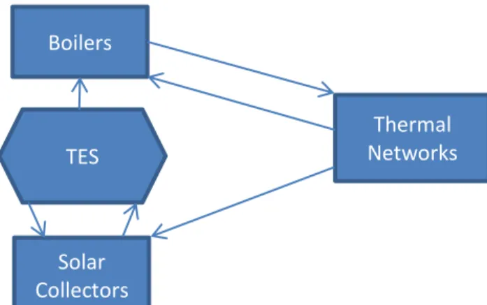
This research focuses on thermodynamic modeling and analysis of the TES in a DE system. Energy and exergy balances and merit measures for TES are described and applied to the TES in the Friedrichshafen DE system. The Friedrichshafen DE system is shown in Figure 1.
Figure 1. Simplified illustration of the Friedrichshafen DE system, showing flows of energy
Energy and exergy balances for a thermal system can be written respectively as (Rosen and Dincer, 2007, 2011):
Energy input – Energy output = Energy accumulation (1) Exergy input – Exergy output – Exergy destruction = Exergy accumulation (2) where
Energy output = Product energy output + Waste energy output (3) Exergy output = Product exergy output + Waste exergy output (4) The energy transferred to a TES is not distributed uniformly when mixing is limited, because vertical thermal stratification develops and the temperature of the storage medium varies spatially. Careful management and utilization of stratification can increase the efficiency and effectiveness of a TES by increasing the exergy stored and recovered.
A stratified TES can be modelled as having a linear temperature distribution model (Dincer and Rosen, 2007; Rosen et al., 2003; Dincer and Rosen, 2007). In such instances, the mixed temperature of the TES Tm can be written as
Tm = (Tt + Tb)/2 (5)
where Tt is the temperature at the top of the TES, and Tb is the temperature at the bottom. The
equivalent temperature of a mixed TES which has the similar exergy as the stratified TES Te can
be expressed as:
Te = exp {[Tt ( ln Tt – 1) – Tb (ln Tb – 1)]/(Tt – Tb)} (6)
Then, the energy of the stratified TES can be expressed:
E = Em = m Cp (Tm – T0) (7) Boilers Solar Collectors s TES Thermal Networks
where Em denotes the energy of the fully mixed storage, m the mass of the water in the TES, Cp
is the specific heat at constant pressure of the storage fluid, and T0 is the reference-environment
temperature. The energy of the stratified and fully mixed storage is the same. Similarly, the exergy of the stratified TES can be expressed as:
Ex = E – mCpT0 ln (Te/T0) (8)
while the exergy for the fully mixed storage can be written as:
Exm = E – mCpT0 ln (Tm/T0) (9)
The exergy of the stratified tank differs from that of the fully mixed tank, which can be expressed as:
Ex – Exm = mCpT0 ln (Tm / Te) (10)
An important assumption here relates to the thermal stratification of the TES. Three temperatures are measured in the TES, and the performance of the TES during the charging, storing and discharging is determined accounting for spatial variations in TES temperature.
Energy and exergy analyses for different seasons are determined for the TES during its three operating stages: charging, storing, and discharging.
TES Charging Stage
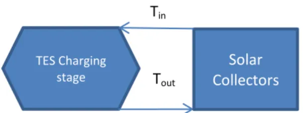
A simplified model of the TES charging stage is illustrated in Figure 2. The extra energy generated by solar collectors in the charging stage is directed to the TES. Water with the lowest temperature, at the bottom of the TES, flows to the solar panels where it is heated and returns to the top of the TES where the temperature is highest.
Figure 2. Charging stage of the TES, where stored energy is provided by solar energy
The general energy balance in equations (1) and (2) can be expressed for the charging phase as: Net energy input – Heat loss = Energy accumulated in TES (11) Qin-TES – Qloss-TES = ∆Uc (12)
where Qin-TES represents net energy input to the TES, Qloss-TES the TES energy loss, and ∆Uc the
energy accumulated in the TES during charging, i.e.,
∆Uc = m Cv ∆Te (13)
Here, ∆Te is the equivalent temperature difference of the TES water in a certain period of time
(defined here as one month), and Cv the specific heat at constant volume of the storage fluid.
Also, the storage mass m is expressible as:
m = ρ V (14) where ρ denotes the density of water in the TES at its temperature and V the volume of the TES.
TES Charging stage Solar Collectors Tin Tout
Heat is transferred by a flow of water to the TES. The mass of the flowing water is determined as follows:
mc =
(15)
where mc is the mass of water transferring energy to the TES during charging, and Tin and Tout
denote the TES inlet and outlet temperatures respectively.
The energy efficiency of the Friedrichshafen TES for charging can be written as:
=
(16)
An exergy balance for the DE system can be written with equations (2) and (4) as:
Exergy input – Exergy destruction – Exergy loss = Exergy accumulation (17) Exergy input = mc [hin – hout – T0 (sin – sout)] (18)
where hin and hout is the specific enthalpy of the inlet and outlet water to/from the TES
respectively, and sin and sout denote the specific entropy of inlet and outlet water to/from the TES
respectively. Also,
Exergyloss charging = Qloss-TES (1 – ) (19)
Exergy accumulation = Exf – Exi = m [uf – ui – T0(sf – si)] (20)
where uf and ui are specific internal energy at the final and initial states of the TES respectively,
sf and si are the final and initial specific entropy of the TES. T0 and Te are in K. Furthermore,
Exergy destruction = mc[hin–hout–T0(sin–sout)] – Qloss-TES(1 – ) – m [uf–ui–T0(sf–si)] (21)
The exergy efficiency of the TES during the charging stage is expressible as:
(22) TES Storing Stage
The storing stage is the interim stage for a TES to store energy without charging or discharging. An energy balance for storing stage is as follows:
–Energy loss = energy accumulation (23) and the energy efficiency of the storing period ηs can be written as:
(24) An exergy balance for the storing stage can be expressed as:
–Exergy loss – Exergy destruction = Exergy accumulation (25) and the exergy efficiency of storing period ψs as:
(26) TES Discharging Stage
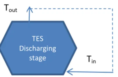
During the discharge stage (see Figure 3), stored energy in the TES is recovered for use in the Friedrichshafen DE system. The dotted line in Figure 3 represents the cycle of water from the
TES through other components of DE system. Here, Qrec denotes the recovered energy from the
TES, Qloss-TES the heat loss from the TES and ∆Ud the energy accumulation of the TES during
discharging, expressible as:
∆Ud = m Cv ∆Tm (29)
During discharging, ∆Ud takes on a negative value.
Figure 3. TES discharging stage, where stored energy is transferred to the DE system
Heat exits the TES via a water cycle. The outlet water flow mass can be evaluated as: md =
(30)
where md is the mass of the transfer fluid, and Tin and Tout denotes temperature of the inlet/outlet
in/from the TES respectively.
The energy efficiency of the TES during discharging is:
=
(31)
where Qloss-d is the heat loss during the discharge stage and Qrec is as defined earlier.
An exergy balance for the TES in the DE system can be expressed with equations (3) and (4) as follows:
– (Exergy recovered + Exergy loss) – Exergy destruction = Exergy accumulated (32) Exrec = md [hout – hin – T0 (sout – sin)] (33)
Here, Exrec denotes the recovered exergy, hout and hin are the specific enthalpy of the TES outlet
and inlet water respectively, and sout and sin represent the specific entropy of outlet and inlet
water from/to the TES respectively. Also,
Exergy loss= Qloss-TES (1 – ) (34)
Exergy accumulation = Exf – Exi = m[uf – ui – T0 (sf – si)] (35)
Exergy destruction = md[hout–hin–T0(sout–sin)] – Qloss-TES(1 – ) – m[uf–ui–T0(sf–si)] (36)
where uf and ui are the final and initial states internal energy of the TES respectively, other
parameters are defined already.
The exergy efficiency of the TES during can be expressed as: (37) TES Discharging stage Tout Tin
TES Overall Cycle
An overall energy balance for the TES of the DE system can be expressed as:
Energy input – (Energy recovered + Heat loss) = Energy accumulation
∑ ∑ ∑ = Ʃ ∆Uc (38)
and the overall energy efficiency of the TES can be written as:
= ∑
∑ (39)
Similarly, we can express an overall exergy balance for the TES of the DE system as: Exergy input–(Exergy recovered+Exergy loss)–Exergy destruction=Exergy accumulation
∑ ∑ ∑ – ƩExdest = ∑ (40)
and the overall exergy efficiency ψo of the TES as: o = ∑ ∑ (41)
3 Description Friedrichshafen DE System and its TES
Nuβbicker-Lux and Schmidt (2005) report that the first phase of the Friedrichshafen DE system included a hot water TES made of reinforced concrete with a volume of 12,000 m3 which served 280 apartments in multi-family houses and a daycare, and included flat plate solar collectors with an area of 2700 m2.Solar heat provided 24% of the total heat demand for district heating. In the second phase, built in 2004, district heating was expanded to a second set of apartments comprising 110 units, and 1350 m2 of solar collector area was added to the system. Also, two gas condensing boilers were installed to cover the energy demand for district heating during periods when insufficient energy is available via the solar collectors and thermal storage.
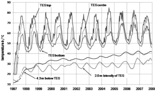
Figure 4. Historical variation of temperatures in and near the TES in the Friedrichshafen DE system(Nuβbicker et al. (2009), printed by permission)
The Friedrichshafen DE system contains two natural gas boilers, solar thermal collectors mostly on building roofs, a central solar heating plant with seasonal heat storage (CSHPSS), heat exchangers to transfer heat between the thermal network and solar collectors, and the thermal network which distributes heat to consumers, as well as pipes, pumps and valves. Water is the heat storage media and the heat transport media circulating in the Friedrichshafen system.
Historical temperature data for the Friedrichshafen DE system (Nuβbicker-Lux and Schmidt, 2005) are presented in Figure 4. Also, data for a typical annual period follows:
- Return water (circulating media) from thermal network temperature: 55.4°C - Measured TES heat loss: 421 MWh
- Storage efficiency: 60%
- Thermal energy yield of solar collectors: 1200 MWh - Solar heat input to district heating network: 803 MWh - Overall heat delivery to district heating network: 3017 MWh - Heat delivered by gas bolilers: 2310 MWh
- Solar fraction: 26%
- Maximum temperature in TES: 81°C (at top)
Note that the temperature of the return water is reported as an annual average, although in the reality the return temperature varies depending on the time of day and season. The temperature and mass flow rate of the water, the building profile, and weather conditions affect the return temperature. Nonetheless, the temperature of the return water is considered constant here to simplify the calculations in this preliminary study, thereby permiting the main objective of assessing the role of the TES to be more clearly illustrated.
Also, Lottner and Mangold (2000) and Fisch and Kubler (1997) report that the temperature of thermal network (T) in average all over the year is 70°C.
For simplicity, it is assumed here, based on a similar thermal system reported by Zhai et al. (2009), that heat losses in pipelines are neglegible.
4 Results and Discussion
Energy and Exergy ParametersThe year 2006 is considered in the present analysis because it appears to be a typical year. Consequently, TES temperature for each season are taken from Figure 4 for that year. Monthly temperatures in and near the TES for 2006 are listed in Table 1, along with the monthly environment temperature (Tutiepo, 2011).
The total energy loss of the TES during 2006, reported to be 421 MWh, needs to be broken down by month. Note that TES in the Friedrichshafen DE system is built in the ground, so heat loss is mostly between the TES and the surrounding soil. Data are available of the soil temperature 4.3 m under the TES. Here, this temperature is assumed for TES heat losses in all directions. Because the volume of underground Friedrichshafen TES is large at 12,000 m3, most of the TES is deep in the ground. Since the temperature of the ground is almost constant at a depth of 10 m, the majority of surrounding soil is thus at a constant temperature, so we use a single ground temperature in all directions here for simplicity. The temperature difference between the TES and the soil 4.3 m below the TES is calculated for each month. The soil temperature is read from Figure 4 and listed in Table 1. Table 1 also contains the breakdown by month and season of the received solar energy, estimated by Rezaie et al. (2012), is also illustrated in Table 1.
Table 1. TES, soil and ambient temperatures during the year 2006 Season/
Solar generation
Month TES temp. (top), °C TES temp. (center), °C TES temp. (bottom), °C T0, °C Soil temp., °C ∆T (Tave – soil temp.), °C Q loss-TES, MWh Spring / 376.07 MWh Mar. 60 56 52 3.4 26 30 32.6 Apr. 70 61 56 9.9 25 36 39.1 May 80 69 60 13.7 25 44 47.7 Summer / 473.33 MWh Jun. 83 74 63 19.8 26 48 52.1 Jul. 82 76 67 19.7 28 48 52.1 Aug. 87 74 66 16.1 31 43 46.7 Fall/ 233.42 MWh Sept. 74 65 58 17.9 34 31 33.6 Oct. 60 59 50 13.0 35 24 26.0 Nov. 54 52 51 6.6 34 18 19.5 Winter / 116.76M Wh Dec. 51 50 48 2.7 32 19 20.6 Jan. 54 52 50 –2.6 30 22 23.9 Feb. 55 54 51 0.3 29 25 27.1 Ʃ=388 Ʃ=421
Legend: ∆T is temperature difference between TES center temperature and soil temperature, Qloss-TES is TES heat loss in each month (estimation is explained in the text).
Sources: Rezaie et al. (2012), and Tutiepo (2011) and Nuβbicker et al. (2009).
Also, the sum of the monthly differences between the centre TES temperature and the soil temperature for the year is 388°C; these values are used as weighting factors in determining the monthly breakdown of the TES annual heat loss. That is, the energy loss for each month is calculated by multiplying its temperature difference by the ratio 421 MWh/388°C. For example, the TES heat loss for March is determined to be:
Q loss-TES =421(30/ 388) = 32.6 MWh (for March)
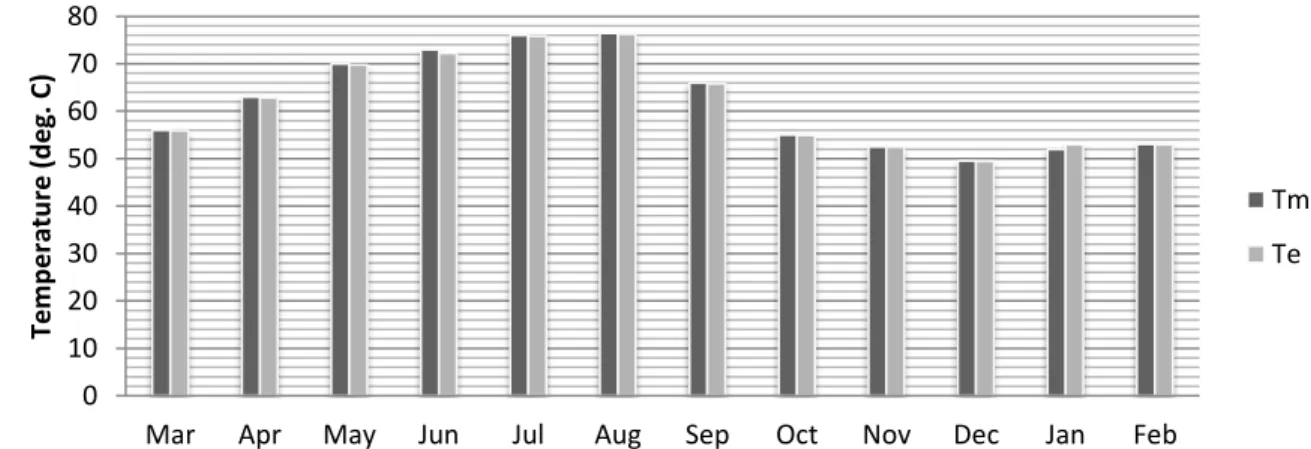
Values for Te and Tm are determined using equations (5) and (6) and values for Tb and Tt
are listed in Table 1. Monthly values of Te and Tm for the Friedrichshafen TES in 2006 are
depicted in Figure 5.
Figure 5. Monthly values for the effective temperature and fully mixed temperature for the TES in the Friedrichshafen DE system for 2006
0 10 20 30 40 50 60 70 80
Mar Apr May Jun Jul Aug Sep Oct Nov Dec Jan Feb
Tem p er atu re (d eg . C) Tm Te
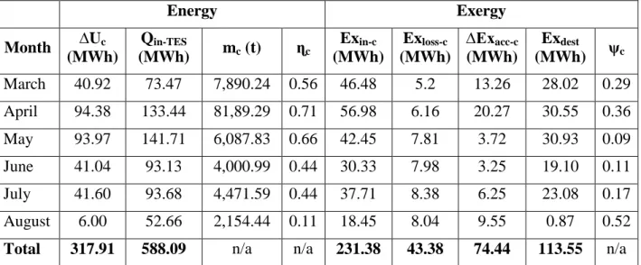
Energy and exergy parameters for the TES, evaluated with equations (12) to (22) during charging months, accounting for thermal stratification, are listed in Table 2. There, the average temperature for the TES charging stage is assumed fixed at 72°C (for which Cp = 4.19 kJ/kg K).
The TES in the Friedrichshafen DE system provides energy for the DE system when the top temperature of the TES is higher than 55.4°C; otherwise the TES does not provide heating. Thus, from Table 1, November, December, January, and February are months when the TES is not used for heating in the Friedrichshafen DE system since in these months TTES < 55.4°C.
Therefore, in Table 3 the rows of November, December, January, and February are not shown. From March to August, ∆Uc and Qin-TES for each month are positive, which means the energy of
the TES is increasing every month compared to the previous month. This pattern is repeated in the exergy section: from March to August the exergy level is increasing relative to the previous month. So, March to August is the charging stage of the TES. The energy and exergy efficiencies of the stratified TES for the overall charging stage are determined using equations (16) and (22) to be 54% and 24%, respectively.
Table 2. Energy and exergy parameters for the Friedrichshafen TES in 2006 during charging, accounting for stratification
Energy Exergy Month ∆Uc (MWh) Qin-TES (MWh) mc (t) ɳc Exin-c (MWh) Exloss-c (MWh) ∆Exacc-c (MWh) Exdest (MWh) ψc March 40.92 73.47 7,890.24 0.56 46.48 5.2 13.26 28.02 0.29 April 94.38 133.44 81,89.29 0.71 56.98 6.16 20.27 30.55 0.36 May 93.97 141.71 6,087.83 0.66 42.45 7.81 3.72 30.93 0.09 June 41.04 93.13 4,000.99 0.44 30.33 7.98 3.25 19.10 0.11 July 41.60 93.68 4,471.59 0.44 37.71 8.38 6.25 23.08 0.17 August 6.00 52.66 2,154.44 0.11 18.45 8.04 9.55 0.87 0.52
Total 317.91 588.09 n/a n/a 231.38 43.38 74.44 113.55 n/a
Legend: ∆Uc: Energy accumulation in TES, Qin-TES: Energy input to TES, m: mass of water
transferring energy, ɳc: Energy efficiency of TES, Exin-c: Exergy input to TES, Exloss-c: Exergy
loss from TES, ∆Exacc-c: Exergy accumulation in TES, Exdest: Exergy destruction for TES, ψc:
Exergy efficiency of TES.
In the storing stage energy loss is equal to energy accumulation. Since the Friedrichshafen DE system TES is not adiabatic, there are always heat losses from the TES. The first month after the charging stage (September), the energy loss exceeds the energy input. Hence, the TES directly shifts from the charging stage to the discharging stage and there is no storing stage for the Friedrichshafen DE system.
It is seen that for September and October ∆Ud has a negative value, meaning the TES is
losing energy compared to the previous month as it discharges energy to the Friedrichshafen DE system. The change in TES exergy is also negative during September and October. Energy and exergy parameters for the stratified TES during the two discharging months, evaluated using equations (28) to (36), are listed in Table 3. For the overall discharging stage, energy and exergy
system, accounting for stratification, as 85% and 41%, respectively. As noted earlier, the TES does not heat the Friedrichshafen DE system from November to February.
For the stratified TES, the overall energy efficiency is determined with equation (39) to be 60% and the overall exergy efficiency ψo is determined with equation (41) to be 19%.
Comparison of Exergy Parameters for Fully Mixed and Stratified Storage
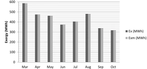
Exergy and energy parameters are determined considering thermal stratification as well as assuming the simpler model of a fully mixed tank at a uniform temperature. The TES energy contents for both situations are the same, but the exergy differs. The difference in the TES exergy content for fully mixed and stratified conditions is equations (8) and (9) for several months (see Figure 6). The differences are small, in line with the fact that the differences between effective temperatures and fully mixed temperature in Figure 5 are also small.
Table 3. Energy and exergy parameters for the Friedrichshafen TES in 2006 during discharging, accounting for stratification
Energy Exergy Month ∆Ud (MWh) Qrec (MWh) md(t) ɳd Exrec (MWh) Exloss-d (MWh) ∆Exacc-d (MWh) Exdest (MWh) ψd Sep. –142.11 175.75 8,118.37 0.84 –24.70 4.76 72.89 43.50 0.34 Oct. –148.93 174.97 32,681.50 0.87 –18.52 3.33 32.75 10.90 0.57
Total –291.04 350.72 n/a n/a –43.15 8.09 105.63 54.39 n/a
Legend: ∆Ud: Energy accumulation in TES, Qrec: Energy recovered by TES, md: mass of water
transferring energy, ɳd: Energy efficiency of TES, Exrec: Exergy recovered by TES, Exloss-d:
Exergy loss from TES, ∆Exacc-d: Exergy accumulation in TES, Exdest: Exergy destruction for
TES, ψd: Exergy efficiency of TES
Figure 6. Comparison of exergy contents of the Friedrichshafen TES for fully mixed and stratified conditions 0 100 200 300 400 500 600
Mar Apr May Jun Jul Aug Sep Oct
Exer gy (M Wh) Ex (MWh) Exm (MWh)
The results suggest that accounting for stratification or simplifying by assuming a fully mixed tank does not significantly affect thermodynamic analyses for the Friedrichshafen TES. This result is likely applicable to other TESs where thermal stratification is not great.
Comparison of Energy and Exergy Performance
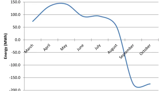
The variation in energy content in the Friedrichshafen TES over an annual period is shown Figure 7. In the charging stage, the energy is increasing in the TES, and in the discharging stage the TES is losing the energy (reflected by negative values in the diagram) as it releases energy to the Friedrichshafen DE system.
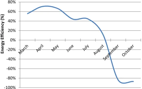
The variation in energy efficiency in the Friedrichshafen TES over an annual period is shown Figure 8. The energy efficiency is positive during charging and negative during discharging. The negative value is related to direction, and means the TES is discharging stored energy to the DE system. Figures 7 and 8 exhibit similar trends. Note that the negative portions of Figures 7 to 10 indicate the behaviour of the TES during discharging whereas the positive portions are for charging. In the charging stage, the TES is accumulating energy and in discharging stage it is releasing energy.
Figure 7. Annual variation in energy content of the TES in the Friedrichshafen DE system
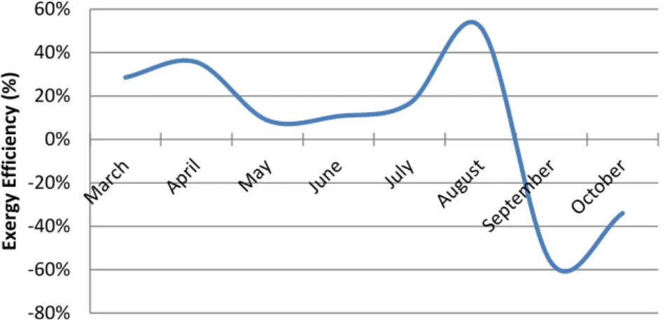
The variation in the exergy accumulation in the TES in the Friedrichshafen DE system over a year is shown in Figure 9. The exergy content of the TES increases during charging, and decreases during discharging as the accumulated exergy is released to the Friedrichshafen DE system. Note in Figure 9 that the exergy accumulation decreases slightly from May to July since the ambient temperature increases and exergy is calculated based on a reference-environment temperature. The variation in exergy efficiency in the Friedrichshafen TES over an annual period is shown Figure 10, which exhibits a similar trend to Figure 9.
-200.0 -150.0 -100.0 -50.0 0.0 50.0 100.0 150.0 En e rg y (M Wh)
Figure 8. Annual variation in energy efficiency of the TES in the Friedrichshafen DE system
5 Conclusions
The TES in the Friedrichshafen DE system has been analyzed, accounting for thermal stratification. Energy and exergy are input to the TES during charging when surplus energy and exergy are harvested by solar collectors, mainly in the spring and summer, and the stored energy and exergy are subsequently discharged to the Friedrichshafen DE system. The overall energy and exergy efficiencies of the stratified TES in the DE system are 60% and 19%, respectively.
Figure 9. Annual variation in exergy accumulation in the TES in the Friedrichshafen DE system, accounting for thermal stratification
-100% -80% -60% -40% -20% 0% 20% 40% 60% 80% En e rg y Eff ic ie n cy (% ) -80.0 -60.0 -40.0 -20.0 0.0 20.0 40.0 Exer gy (M Wh)
Figure 10. Annual variation in exergy efficiency of the TES in the Friedrichshafen DE system, accounting for thermal stratification
The analysis results (e.g., energy and exergy contents and efficiencies) for the TES in the Friedrichshafen DE system when stratification is accounted for are similar to those when a fully mixed assumption is applied. The results suggest that accounting for stratification or simplifying by assuming a fully mixed tank does not significantly affect thermodynamic analyses for TESs with moderate thermal stratification, as is the case for the Friedrichshafen TES.
6 Acknowledgment
Financial support provided by the Natural Sciences and Engineering Research Council of Canada is gratefully acknowledged.
7 References
Casten, T. R., Ayers, R. U. 2005. Recycling Energy: Growing Income while Mitigating Climate
Change. Report, Recycled Energy Development, Westmont, IL, Oct. 18. Available online
at: http://www.recycled-energy.com/_documents/articles/tc_energy_climate_ change.doc. [Accessed 27 Oct. 2011]
Dincer, I., Rosen, M., 2011. Thermal Energy Storage: Systems and Applications. 2nd edition, Wiley.
Dincer, I., Rosen, M., 2007. Exergy: Energy, Environment and Sustainable Development. Elsevier.
Dincer, I., 2003. On energy conservation policies and implementation practices. International Journal of Energy Research, 27: 687-702.
Fisch, N., Kubler, R., 1997. Solar assisted district heating-status of the projects in Germany. International Journal of Sustainable Energy, 18: 259-270.
Kharseh, M., Nordell, B., 2011. Sustainable heating and cooling systems for agriculture. International Journal of Energy Research 35: 415-422.
-80% -60% -40% -20% 0% 20% 40% 60% Exer gy E ff ic ie n cy (% )
Lottner, V., Mangold, D., 2000. Status of seasonal thermal energy storage in Germany. Proc. 8th Int. Conf. on Thermal Energy Storage, Stuttgart, Germany, August 20–September 1, Vol. 1, pp. 53-60.
Marinova, M., Beaudry, C., Taoussi, A., Trepanier, M., Paris, J. 2008. Economic assessment of rural district heating by bio-steam supplied by a paper mill in Canada. Bulletin of Science, Technology & Society, 28 (2): 159-173.
Nuβbicker, J., Bauer, D., Marx, R., Heidemann, W., Muller-Steinhagen, H. 2009. Monitoring results from German central solar heating plants with seasonal storage. Proc. EFFSTOCK 2009, Stockholm, Sweden, June 14-17.
Patil, A., Ajah, A., Herder, P., 2009. Recycling industrial waste heat for sustainable district heating: A multi-actor perspective. Int. J. Environmental Technology and Management, 10: 412-426.
Rezaie, B., Reddy, B. V., Rosen, M. A. 2012 (in press). Role of thermal energy storage in
district energy systems. Chapter 15 in Rosen, M. A. (Ed.), Energy Storage, NOVA
Publishers, New York, USA.
Rezaie, B., Rosen, M.A., 2012. District heating and cooling: Review of technology and potential enhancements. Applied Energy 93: 2-10.
Robins, J., 2010. The New Good Life: Living Better than Ever in an Age of Less. Ballantine Books.
Rosen, M. A. 2009. Combating global warming via non-fossil fuel energy options. International Journal Global Warming 1 (1-3): 2-28.
Rosen, M. A., Dincer, I., Kanoglu, M., 2008. Role of exergy in increasing efficiency and sustainability and reducing environmental impact. Energy Policy 36: 128-137.
Rosen, M.A., Dincer, I., 2003. Exergoeconomic analysis of power plant operating on various fuels, Applied Thermal Science 23: 643-658.
Rosen, M. A., Dincer, I., 1999. Exergy analysis of waste emissions. International Journal of Energy Research 23:1153-1163.
Rosen, M. A., Dincer, I., 1997. On exergy and environmental impact. International Journal of Energy Research 21: 643-654.
Rosen, M. A., Tang, T., Dincer, I., 2003. Effect of stratification on energy and exergy capacities in thermal storage systems. International Journal of Energy Research 28: 177-193.
Tutiempo. 2011. Historical Weather: Friedrichshafen, year 2006. Available on line at:
www.tutiempo.net/en/Climate/Friedrichshafen/109350.htm [Accessed Oct, 15, 2011]
Zhai, H., Dai, Y. J., Wu, J. Y., Wang, R. Z., 2009. Energy and exergy analyses on a novel hybrid solar heating, cooling and power generation system for remote areas. Applied Energy 86: 1395-1404.