Counting Network Flows over Sliding Windows

(1)

Counting Network Flows over

Sliding Windows

Josep Sanju`as Cuxart – [email protected]

Pere Barlet Ros – [email protected]

UPC Technical Report

Deptartament d’Arqutiectura de Computadors

(2)

Abstract

Counting the number of flows present in network traffic is not trivial, given that the naive approach of using a hash table to track the active flows is too slow for the current backbone network speeds.

Several probabilistic algorithms have been proposed in the recent literature that can calculate an approximate count using small amounts of memory and few memory accesses per packet. Fewer works have addressed the more complex problem of counting ﬂows over sliding windows, where the main challenge is to continuously expire old information. One of the existing proposals is a straightforward adaptation of a technique called linear-time probabilistic counting to the sliding window model.

We present an algorithm called Countdown Vector that also builds upon linear count-ing. We perform a thorough experimental validation of the accuracy of our algorithm and compare its cost to the state of the art. Our algorithm obtains signiﬁcant cost reductions both in terms of memory and CPU utilization, by introducing an extra approximation in the mechanism in charge of the expiration of old information.

(3)

Chapter 1

Introduction

The design of efficient algorithms to count the number of active flows in high-speed networks has recently attracted the interest of the network measurement community [1, 2, 3]. Counting the number of flows in real-time is particularly relevant to network operators and administrators for network management and security tasks. For example, this metric is the basis of most network intrusion detection systems, such as Snort [4] or Bro [5], to detect port scans and DoS attacks.

However, the naive solution of tracking flows using a hash table is becoming unfeasible in high-speed links. First, it requires several memory accesses per packet with the overhead of creating new flow entries and handling collisions. Second, this solution uses large amounts of memory, since it requires storing all flow identifiers. The number of concurrent flows present in high speed networks is very large, and can be well over one million in current backbone links [6]. Therefore, hash tables must be stored in DRAM, which has an access time greater than current packet interarrival times. For example, access times of standard DRAM are in the order of tens of nanoseconds, while packet interarrival times can be up to 32 ns and 8 ns in OC-192 (10 Gb/s) and OC-768 (40 Gb/s) links respectively. Thus, flow counting algorithms must be able to process each packet in very few nanoseconds to be suitable for high-speed links.

In order to reduce the large amount of memory required to store flow tables, most routers (e.g., Cisco NetFlow [7]) and network monitoring systems [8] resort to packet sampling. However, it has been shown that packet sampling is biased towards large flows and tends to underestimate the total number of flows [9].

Recently, several probabilistic algorithms have been proposed to efficiently estimate the number of flows in high-speed networks [1, 2, 3]. These algorithms share the common approach of using specialized data structures to approximately count the number of flows, which need a very small amount of memory, as compared to the traditional approach of keeping per-flow state, while requiring one or very few memory accesses per packet. This drastic reduction in the memory requirements allows the storage of these data structures in fast SRAM, with access times below 10 ns. These techniques can therefore be implemented in router line cards or, in general-purpose systems, the data structures can reside in cache memory.

(4)

Linear-time probabilistic counting is the basis of many probabilistic algorithms to estimate the number of ﬂows. This technique was proposed by Whang et al. [10] in database research, and was popularized in the networking community by Estan et al. in [1] under the name direct bitmaps.

The basic idea behind direct bitmaps is to use a small vector of bits (i.e., bitmap). For each packet, a hash of the flow identifier is computed and the corresponding bit is set in the bitmap. At the end of a measurement interval, the number of flows can be simply estimated according to the number of non-set bits and the collision probability [10]. The main problem of these algorithms is that they can only operate over fixed, non-overlapping measurement intervals and, therefore, cannot obtain continuous estimates of the number of flows.

The sliding window model is increasingly gaining interest in the networking and database communities, given the streaming nature of many current data sources (e.g., network traffic, sensor networks or financial data). Under this new paradigm, queries process streaming data, instead of static databases, and compute metrics over time windows that advance continuously (e.g., the number of active flows during the last 5 minutes).

The principal problem when calculating a metric over a sliding window is how to expires old information as it ages out of the window. Kim and O’Hallaron [3] propose a technique that addresses the flow counting problem called Timestamp Vector (TSV). The TSV is based on probabilistic counting, and essentially consists of replacing the bitmap for a vector of timestamps. The main limitations of the TSV are that (i) it requires a significantly larger amount of memory compared to the original direct bitmap (a 64-bit timestamp for each vector position) and (ii) the cost of the queries is linear with the size of the vector, which renders this solution impractical in scenarios where a continuous estimate of the number of flows is needed.

In this work, we propose a new algorithm called Countdown Vector to estimate the number of ﬂows over sliding windows. The basic idea behind our method is the use of a vector of small timeout counters, instead of full timestamps, that are decremented independently of the per-packet update and query processes. Our algorithm is lighter in terms of both CPU and memory usage than existing solutions, and hasO(1) query cost. Thus, a network monitoring system can implement our method using less memory, and can react faster to changes in the number of ﬂows (e.g., network anomalies or attacks), since queries can be issued more frequently than in previous proposals. Another interesting advantage of our technique over other alternatives is that it is possible to degrade the accuracy of the estimates according to a given CPU and memory budget.

We implement our algorithm in an existing network monitoring system and present experimental evidence of the accuracy and cost of our technique using real-world packet traces. Our results show that our technique is able to estimate the number of ﬂows over a wide range of sliding windows with a similar accuracy to the TSV, while reducing the memory requirements to up to 1/20th and the number of memory accesses to up to 1/30th.

The rest of the document is organized as follows. Chapter 2 introduces the back-ground of the topic. Chapter 3 reviews the Timestamp Vector technique, and presents an

(5)

extension of this technique to reduce its memory requirements, while chapter 4 presents our algorithm to estimate the number of ﬂows over sliding windows. Chapter 5 presents a performance evaluation of our techniques using real packet traces collected at the ac-cess link of a large university network. Finally, chapter 6 concludes and discusses future work.

(6)

Chapter 2

Background

2.1 Network monitoring

The Internet has experimented an exponential growth over the last years. As a con-sequence of the complexity of operating and managing large networks, operators are deploying network monitoring systems to gain an insight on the traffic that traverses net-work links. The information that these monitoring systems obtain can aid in tasks such as traffic engineering, capacity planning, traffic accounting and classification, anomaly and intrusion detection, fault diagnosis, troubleshooting and performance evaluation.

There exist two families of network monitoring techniques. Active network monitor-ing tools inject traffic in a network, and infer properties of the network by collectmonitor-ing said traffic after it has traversed the network. Examples of these techniques range from simple reachability tests (e.g., ICMP pings) to more complex bandwidth estimation tools (e.g., [11]). In contrast, passive network monitoring techniques rely on the analysis of a copy of the traffic that traverses network links. Traffic can be replicated by physical means (e.g., optical splitters or Ethernet taps) or using specialized features of network hardware (e.g., the port span feature present in most Cisco [12] switches and routers). The copy of the traffic is then fed to the passive network monitoring system, which can then compute any metric of interest via per-packet analysis.

Active network monitoring tools are generally easier to deploy, since they do not require modification to the network infrastructure in order to replicate packets, but instead are installed on end-hosts. In contrast, they are more invasive in that they require injecting traffic in the network that can interfere with its normal operation. On the other hand, passive network monitoring offers a direct vision of the traffic that traverses a network link, enabling per-packet analysis.

The most challenging aspect of passive network monitoring systems is that they operate under heavy resource constraints. Due to the ever-increasing bandwidth of network links, and, especially, backbone network links, they have little time to process each incoming packet. Also due to the massive data rates, buffering for long periods of time is impractical. Therefore, network traffic has to be processed in strict real time. Failure to do so results in buffer overflow, which in turn leads to packet losses that

(7)

impact severely on the measurement accuracy of the monitoring system.

This challenge can be approached in two complementary ways. One is to incorporate load shedding mechanisms that can reduce the load of the system when facing overload, usually by applying traﬃc sampling. The other is to design specialized algorithms to calculate the metrics of interest very eﬃciently.

We have in the past tackled the research challenge of load shedding in network monitoring systems [8, 13]. In this work, we are concerned with a particular metric: counting network flows over a sliding window. Instead of simply resorting to sampling, we propose an extremely efficient algorithm to calculate this metric and, in any case, traffic sampling is left as a second line of defense of the network monitoring system against overload.

2.2 Data stream processing

The problem of data stream processing has recently attracted much attention in the database community. The stream processing model assumes, instead of the traditional static data set, that data flows continuously from a source. The system, thus, cannot control the input data rates. Also, data streams are potentially unbounded in size, which impedes storing the whole dataset. Therefore, algorithms can perform only one single pass on the data. Examples of data streams are network traffic, information from sensors and financial data, their key characteristic being the large volume and data rates, that impede storing a copy of the data in memory. Processing a data stream requires algorithms that can operate with a single pass on the data. Interesting introductions to the field of data streams research can be found in [14] and [15]. A more informal discussion of the motivations behind this research area is [16].

2.3 Counting network ﬂows

The problem of counting flows in network traffic is equivalent to that of counting distinct elements within a multiset, where the distinct elements to be counted are the flow identi-fiers. This problem has received attention from the database research community. Many algorithms have been proposed that can obtain approximate distinct element counts over a large dataset by using little memory, requiring one single pass over the data, and with extremely low computational complexity. This problem was first explored in database research, where these algorithms were used for database query optimization [17].

Especially relevant to us is the proposal by Whang el al [10]. Linear-time probabilistic counting is based on pseudo-random hashing. The ratio of buckets that would have stayed empty on a hypothetical hash table is used to estimate the number of unique elements in the original dataset. This algorithm was popularized under the name direct bitmaps in the networking community by Estan et al. [1], along with several variants that increase memory eﬃciency, including multi-resolution bitmaps. An algorithm called Loglog counting of similar eﬃciency to multi-resolution bitmaps is proposed in [18]. Giroire’s proposal [19] is based on estimating cardinalities from the minimum of the

(8)

hashed values. These and other proposed algorithms are compared in [20]. A remarkable conclusion from this study is that, while direct bitmaps are theoretically slightly inferior to its competitors, they are the most practical choice, given their overall good accuracy, extreme speed and ease of implementation.

2.4 The sliding window model

Usually, an analyst is not interested on calculating a metric across the whole stream’s lifetime. The latest data of the stream is often more relevant than the older data. Several models exist to capture this notion of interest decay. The most relevant to us is the sliding window model, where data older than a certain age is completely irrelevant. This and other interest decay functions are analyzed in [21].

Interest decay functions, including the sliding window model, introduce an extra layer of complexity to algorithms, in that they must take into account the aging of information, and expire it accordingly. For example, when tracking the number of ﬂows over a sliding window using a hash table, each entry would additionally require an expiration timestamp, and the algorithm should discount old entries when calculating its result.

Many eﬃcient specialized algorithms to extract statistics over a sliding window have been proposed. Datar et al. [22] analyze the basic problem of counting the number of ones within the last N elements of an arbitrary stream composed of zeros and ones. They present an algorithm based on a technique called Exponential Histograms that can provide an approximate solution, and prove its optimality in terms of memory usage. They then proceed to solve, using their basic counting algorithm as a building block, similar problems such as calculating sums, averages, maximum and minimum values and distinct counts. For the distinct count problem, they propose adapting probabilistic counting techniques to the sliding window model by storing timestamps instead of bits in each bitmap position, an approach that [3] also takes.

Fusy and Giroire present in turn an adaptation of the previously introduced pro-posal [19] to the sliding window model in [2]. Their algorithm tracks the minimum of the hashes of each flow identifier over a sliding window to estimate the flow count.

Kim et al. adapt direct bitmaps [1] to the sliding window model in [3]. Their proposal is to change the bitmap for a vector of timestamps. Instead of storing zeros and ones, each position holds the timestamp of the last packet whose flow identifier hashed to the corresponding position. The algorithm can then provide an estimate of the number of flows by traversing the array and counting the number of positions that were not used within the time window, analogously to [10].

The algorithms we present in chapters 3 and 4 is also an adaptation of direct bitmaps to the sliding window model. Thus, we dedicate sections 3.1 to explain the base linear counting technique from [10], and section 3.2 to the the timestamp vector algorithm.

(9)

Chapter 3

Extending the Timestamp Vector

algorithm

3.1 Linear-time probabilistic counting

Several well-known techniques for efficiently counting flows in network traffic exist in the literature. One of the simplest, yet a very effective one when accounting for complexity and accuracy tradeoffs [20], is the direct bitmaps algorithm presented in [1], originally proposed in the database research field [10] with the name linear-time probabilistic counting. In the rest of this document, we will use the terms direct bitmaps and linear counting interchangeably.

Since both the method we propose in this work and the Timestamp Vector algorithm are a adaptations of linear counting to a sliding window model, we devote this section to explain this technique in greater detail.

A very naive algorithm to count flows can be implemented by using a hash table. Upon receiving a packet, the flow identifier is extracted and looked up in the table. If an entry for the flow identifier does not exist, one is created. The number of flows observed in the traffic then corresponds to the number of entries in the hash table.

There exist two fundamental reasons why the naive algorithm of counting flows using a hash table is impractical. The first is the large memory requirements that it presents when dealing with a massive dataset, since it requires one hash table entry per flow. The second is that this algorithm would require several memory accesses per packet, thus limiting the rates at which data can be processed, which is of importance when dealing with e.g. real-time network traffic.

Like the naive algorithm of using a hash table to track flows, linear counting is based on hashing, but does not maintain one table entry per flow. Instead, it uses a bitmap where it records whether a position in the hash table would be used or not (hence the name bitmap). The algorithm uses a pseudo-random hash function (e.g., [23]) to evenly distribute the positions corresponding to each flow identifier.

Intuitively, all the packets that belong to the same flow hash to the same position in the table, since they share the same flow id. Therefore, each flow activates, at most, one

(10)

Algorithm 1: Linear counting: per-packet operations Data: b: bitmap size

z←b; 1 bitmap← {0, . . . ,0}; 2 foreachpacket p do 3

key←hash(p.ﬂow identiﬁer);

4

if bitmap[keymodb] = 0then /* update count of zeros */

5

z←z−1;

6

end 7

bitmap[keymodb]←1;

8 end 9

Algorithm 2: Linear counting: query procedure

Data: b: bitmap size, z: number of zeros in the bitmap return b ×ln(b/z);

1

position in the bitmap. However, one cannot simply assume that the number of ones in the bitmap corresponds to the number of observed ﬂows, since several network ﬂows can collide, that is, hash to the same position in the bitmap.

While the bitmap cannot be used to extract the exact count of flows, instead, an estimate can be obtained from the bitmap size (b) and the number of zeros in the bitmap (z) as shown in [10, 1] (hence the name linear-time probabilistic counting: only an estimate of the original count can be obtained). Each flow hashes to a particular position with probability 1/b. Given n flows, the probability that no flow hashes to a particular position is (1−1/b)n ≈ e−n/b. Therefore, E[z] ≈ be−n/b. Intuitively, given

z, one can obtain an estimate ofn by solving this equation. Whang et al. [10] formally derive Equation 3.1 and show that it is the maximum likelihood estimator for the number of ﬂows: ˆ n=b ln ( b z ) (3.1)

(11)

Table 3.1: Notation: linear counting

b: Number of positions of the bitmap.

n: Number of ﬂows seen during a measurement interval.

ˆ

n: Estimation of the number of ﬂowsn.

z: #positions with value 0 in the bitmap.

We refer to the process of obtaining an estimate of the number of ﬂows as the process of querying the bitmap. Algorithms 1 and 2 detail the update and query procedures, while table 3.1 summarizes the notation used in this text.

The principal advantage of this technique is that, with a small amount of memory (especially when compared to the naive algorithm), the number of ﬂows can be estimated with high accuracy. A second important characteristic of this approach is that the accu-racy can be arbitrarily increased or reduced by the bitmap size. To correctly dimension the bitmap, the appropriate size must be chosen so that the expected amount of unique elements can be estimated within the desired error bounds, as explained in [10].

To give the reader an idea of how little memory this algorithm requires, it suﬃces to state that this technique can count 106 elements by using around 20KB with an accuracy of 1% [10].

3.2 The Timestamp Vector algorithm

As discussed, direct bitmaps are a very efficient technique to count the amount of flows in the network traffic. However, in order to provide meaningful values when monitoring a network traffic stream, measurement statistics must be bounded in time, i.e., must correspond to a particular time window. Direct bitmaps do not incorporate a sense of time and thus must be periodically reset to avoid lifetime flow counting.

Periodically querying and resetting a direct bitmap would provide ﬂow counts over consecutive, non-overlapping windows. While there is value to this application of the technique, it imposes the restriction that queries must be aligned with bitmap resets. In contrast, in the sliding window model, queries for a measurement interval can arrive at any time. This requirement implies that old information must be removed as newer arrives, in order to continuously maintain the data structures to be able to provide an estimate at any time.

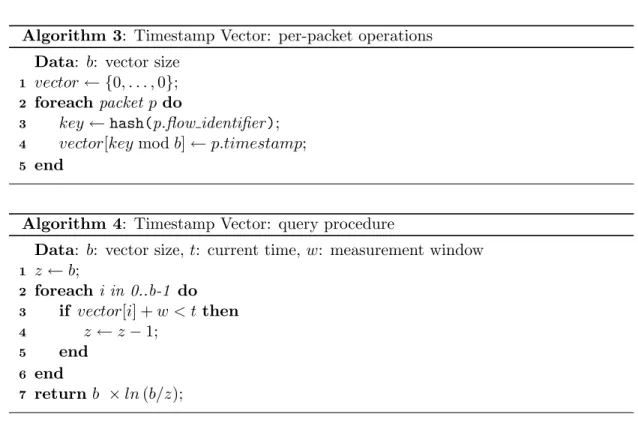
A straightforward solution to adapt the direct bitmaps to the sliding window model is the Timestamp Vector (TSV) algorithm [3]. Instead of a bitmap, a vector of timestamps is now used. When a packet hashes to a particular position, its timestamp is set to the timestamp of that packet. Using this vector, when a query for a time window ofwtime units arrives at time t, the number of ﬂows can be estimated by using Equation 3.1, where in this case z corresponds to the number of positions with timestamp less than

(12)

Algorithm 3: Timestamp Vector: per-packet operations Data: b: vector size

vector← {0, . . . ,0};

1

foreachpacket p do 2

3

vector[keymodb]←p.timestamp;

4 end 5

Algorithm 4: Timestamp Vector: query procedure

Data: b: vector size,t: current time, w: measurement window

z←b; 1 foreachi in 0..b-1 do 2 if vector[i] +w < t then 3 z←z−1; 4 end 5 end 6 return b ×ln(b/z); 7

traversal of the vector for each query. Algorithms 3 and 4 detail the update and query procedures for the TSV.

3.3 Extension of the Timestamp Vector

The principal limitation of the Timestamp Vector technique is the increase in the amount of memory that it requires. Timestamps in network monitoring are typically 64 bits long, e.g. as provided by libpcap [24] or Endace DAG cards [25]. Hence, the ﬁnal size of the vector is increased by a factor of 64 compared to the original bitmap.

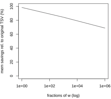
A relaxation of the sliding window model is thejumping window model [26], where the window does not advance continuously, but discretely in fractions of the measurement window. When operating under this model, we propose the following improvement over the Timestamp Vector algorithm that signiﬁcantly reduces its memory requirements. Instead of full timestamps, only the fraction of the window where the packet arrived is stored.

At ﬁrst sight, only w/f diﬀerent values would need to be stored in each vector position. However, an additional value that corresponds to an “out of window” status is necessary. This idea can be trivially implemented usinglog2(w/f + 1) bits per position

when measuring a window ofw time units with query periods off.

Figure 3.1 shows the memory savings that this variant of the TSV achieves. For example, with a window of 30 s and queries every 1 s, the original Timestamp Vector will require 64 bits per position, while this approach would require only 5 bits per

(13)

1e+00 1e+02 1e+04 1e+06 0 20 40 60 80 100 fractions of w (log)

mem savings rel. to original TSV (%)

Figure 3.1: Memory savings of our extension compared to the original Timestamp Vector. The x axis indicates the window jump interval expressed in fractions of the measurement window (notice logarithmic axis).

position, saving over 90% of the memory. Note however that, using this extension, the Timestamp Vector can only be queried everyf time units, in this case, 1 second.

One limitation of both variants of the Timestamp Vector algorithm is, thus, their additional memory requirements. The jumping window variant reduces memory usage by limiting the time where queries may be performed. The second disadvantage of this scheme is that, for each query, one full traversal of the array is required to calculate the number of positions whose timestamp is older than t−w.

(14)

Chapter 4

The Countdown Vector algorithm

In this chapter, we present our technique for ﬂow counting over sliding windows. Our scheme is, like the Timestamp Vector (TSV) algorithm, an adaptation of the direct bitmaps to the sliding window model. We start by outlining the basic intuition behind the technique we propose.

4.1 Intuition

The main diﬃculty when adapting the direct bitmap to the sliding window model is to remove old information from the data structure as time advances. Let us start by deﬁning an ideal algorithm which would precisely calculatez in a sliding window ofw

time units. Recall that b(vector size) and z (number of zeros in it) suffice to estimate the number of flows in the traffic using Equation 3.1. A vector ofb positions could be used, with the values set towtime units every time a packet hashed to the corresponding position. Every time unit, all the positions of the vector with non-zero value would be decremented by one. The count of positions with counter value zero would correspond tozin order to estimate the number of flows seen in the time window.

In order to obtain a perfect resolution, this scheme would require deﬁning the time unit to the maximum resolution of the system clock. This ideal scheme would therefore be very costly in terms of both memory and CPU. First, a high resolution counter would have be stored in each vector position, thus increasing the overall memory required to store the vector. Second, all of the counters would need to be updated for each time unit. These additional costs make this technique infeasible as described, especially when it would achieve results equivalent to the TSV.

The technique that we propose is very similar to the ideal algorithm just described but, instead, using small integer counters in each position. Using small values requires less memory and calls for a low counter decrement frequency for counters to reach zero after w time units, in exchange of introducing small inaccuracies. In the following paragraphs we describe our technique with detail. The key to the effectiveness of our algorithm is that surprisingly low values suffice to achieve good accuracy to estimate network flow counts. In practice, then, we require less memory and introduce lower

(15)

Table 4.1: Notation

b: Number of positions of the vector or bitmap.

c: Value to which counters are initialized.

f:Time between queries in a jumping window model.

n:Number of ﬂows seen during a time window.

ˆ

n:Estimation of the number of ﬂowsn.

s: Time between counter updates.

w:Length of the time window.

z: #positions with value 0 in the bitmap or vector.

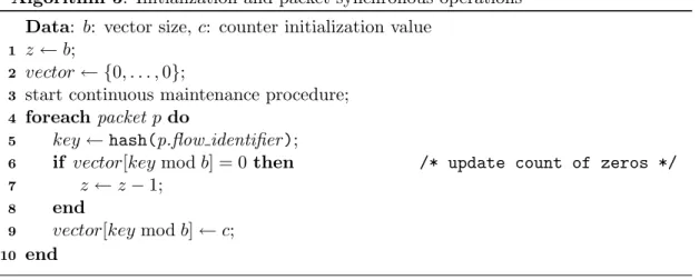
Algorithm 5: Initialization and packet-synchronous operations Data: b: vector size, c: counter initialization value

z←b;

1

vector ← {0, . . . ,0};

2

start continuous maintenance procedure; 3

foreach packetp do 4

5

if vector[keymodb] = 0then /* update count of zeros */

6

z←z−1;

7

end 8

vector[keymodb]←c;

9 end 10

overhead compared to the original TSV algorithm and to its extension presented in Section 3.3.

4.2 Algorithm

Our algorithm starts by allocating a vector of counters, all of which are initialized to zero. Our algorithm can then be seen as divided in two concurrent processes: the ﬁrst updates the vector for each packet, while the second is in charge of decreasing the counters at a ﬁxed rate.

The ﬁrst process is described in Algorithm 5 and runs synchronously with the packet stream. When a packet hashes to a position, we store a maximum value c in the cor-responding position. This process remains the same independently of the time window that is being measured.

In contrast, the second process, which is described in Algorithm 6, performs a contin-uous maintenance of the vector. It decreases one counter everystime units, advancing one position in the vector at every step. The desired time windowwplays a role in this

(16)

Algorithm 6: Continuous maintenance procedure

Data: b: vector size,c: counter initialization value, vector: vector of counters,

z: count of positions with value 0

s← _b_×₍w_c₋1 2) ; 1 i←0; 2 whileTrue do 3

sleep for s time units; 4

if vector[i] = 1then /* update count of zeros */

5

z←z+ 1;

6

end 7

vector[i]←max(0, vector[i]−1);

8

i←(i+ 1) modb; 9

end 10

Algorithm 7: Query procedure

Data: b: vector size,z: number of zeros invector

return b ×ln(b/z); 1

data structure maintenance process, where it conditions the speed at which counters are decreased.

4.3 Parametrization

To determineswe proceed as follows. Since the packet arrivals and the maintenance are independent processes, and each flow hashes to a random position, on average, the first decrement of a counter (after it is set to w by the first process) will happen after b/2 counter updates. Afterwards, the counter will be decremented afterbadditional counter updates. Therefore, on average, counters reach zero afterb/2 +b (c−1) =b (c−1/2) updates. Since this time must correspond to the time window w, we calculate s the following way:

s= w

b(c−1₂) (4.1)

Both the ﬁrst and the second processes maintain the count of positions of the vector with value zero, updating the value of z as values of the vector are modiﬁed. This has the advantage that query operations run in constant timeO(1), by simply applying Equation 3.1, as described in Algorithm 7.

Our algorithm is then governed by the following conﬁguration parameters: (i) the desired measurement window w, (ii) the size of the vector b, and (iii) the maximum values to which counters are setc.

(17)

of b (vector size) make the estimation error of Equation 3.1 decrease, as explained in further detail in [10]. On the other hand, increasingc also has a positive impact on the accuracy of the method, since, the larger c is, the more our algorithm approaches the ideal algorithm explained in the previous subsection.

However, larger values ofcincrease both the memory and CPU requirements of our algorithm, since, the higher c is, the more space is required to store the counters, and the higher the counter decrease frequency, i.e.,sdecreases, according to Equation 4.1.

Our algorithm has two sources of error. First, the approximation introduced by the original technique upon which ours builds, the direct bitmaps. The second source of error is introduced by the fact that old information is expired after w time units only

on average. Inevitably, some counters will, on the worst case, be set to c right after the maintenance process has decremented the corresponding position, and will thus will reach zero after c∗b∗s = _c₋c₁_/₂w time units. Conversely, others will reach zero after

c−1

c−1/2wtime units. In the worst case a counter will be inaccurate only during this small

period of time. This explains why the accuracy increases with larger values ofc, which tighten these bounds aroundw.

In order to choose a value for b, the tables provided by [10] can be looked up to determine the an appropriate vector size for the expected number of ﬂows in the traﬃc. In the next section we analyze the impact of c over the accuracy of the method and show the overhead reduction of our method compared to both variants of the Timestamp Vector.

(18)

Chapter 5

Evaluation

5.1 Experimental setting

In order to obtain sensible results, we have tested our technique using three real 30 min-utes long traffic traces collected both at our University and by the NLANR project [27]. The first two traces, which we callnov2007 and apr2008, were collected during Novem-ber 2007 and April 2008 at the access link of the Technical University of Catalonia (UPC), which connects 10 campuses, 25 faculties and 40 departments to the Internet through the Spanish Research and Education network (RedIRIS). Table 5.1 summarizes the characteristics of the traces we are using for the evaluation. To give the reader an idea of the volume of traffic that this link supports, thenov2007 trace accounts for 106M packets, with an average data rate of 271 Mbps and a peak rate of 399.0 Mbps. The average number of active flows is around 50000 in a ten seconds window, and 1.8 million in a 10 minute window.

As already stated, we also use a trace from the NLANR project [27], which we call

nlanr2005. This trace is older and contains a smaller volume of traﬃc, but has the

advantage of being publicly available, and thus the results presented in this evaluation are independently veriﬁable. We use the ﬁrst 30 minutes of the CENIC-I trace, collected during March 2005.

Trace name Start Time (UTC+1) Duration Packets Bytes Avg traﬃc apr2008 Apr 21, 2008 17:30 30 min. 102.6 M 56.89 GB 258.95 Mbps nov2007 Nov 6, 2007 16:30 30 min. 106.0 M 59.7 GB 271.6 Mbps nlanr2005 Mar 18, 2005 01:00 30 min. 58.31 M 50.70 GB 230.74 Mbps

(19)

5.2 Accuracy results

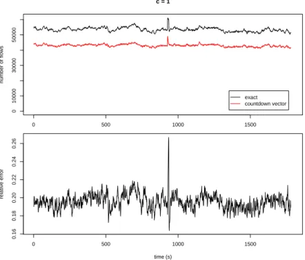
We start by analyzing the timeseries of the execution of three different configurations of thecparameter of the Countdown Vector algorithm to measure the number of active flows in a 10s window, using trace nov2007. Recall that c is the value to which vector values are set to when a packet hashes to the corresponding position.

Figure 5.1 uses c = 1. We can observe that the estimations that the algorithm provides are very poor, and always below the actual values. This is becausec is so low that the algorithm needs to reset the positions of the vector too aggressively, leading to ﬂows that are in fact active being expired before the next packet can top up the associated vector position.

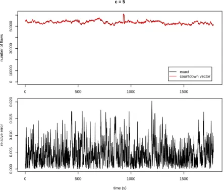
Instead, ﬁgure 5.2 instead, uses c = 5. Using this value, the algorithm no longer systematically underestimates the number of ﬂows, but, instead, provides very accurate estimates, as can be seen in the plot of the relative errors.

Finally, ﬁgure 5.3 uses c= 10. Interestingly, using a counter twice as large does not provide any beneﬁt in terms of increased accuracy, while it would incur a much larger CPU overhead, since positions of the vector need to be decreased more frequently.

0 500 1000 1500 0 10000 30000 50000 c = 1 number of flows exact countdown vector 0 500 1000 1500 0.16 0.18 0.20 0.22 0.24 0.26 time (s) relative error

(20)

0 500 1000 1500 0 10000 30000 50000 c = 5 number of flows exact countdown vector 0 500 1000 1500 0.000 0.005 0.010 0.015 0.020 time (s) relative error

Figure 5.2: Timeseries of the Countdown Vector with c= 5

0 500 1000 1500 0 10000 30000 50000 c = 10 number of flows exact countdown vector 0 500 1000 1500 0.000 0.005 0.010 0.015 0.020 time (s) relative error

(21)

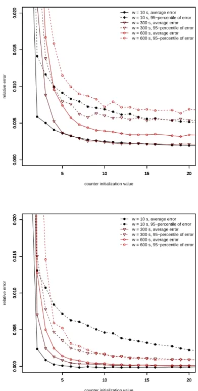
We now perform a set of executions to analyze the impact of c on different window sizes. Figure 5.4 (top) shows the results of running our algorithm on thenov2007 trace with window sizes of 10, 300 and 600 seconds with different counter initialization values, using a fixed vector size. The size of the vector has been chosen according to [10] so that the average number of flows for the largest window can be counted with errors below 1%. Each point in the figure corresponds to a full pass on aforementioned trace, querying the algorithm every second, and shows either the average relative error or the 95th percentile of the relative error compared to a precise calculation of the number of flows.

As expected, for every window size, the relative error decreases as c increases. It is interesting to observe that, while the error is intolerable for very small values of c

(5 and below), when it reaches values as small as 10 the error stabilizes, and does not decrease signiﬁcantly beyond that point, even for a window as large as 600 s. This observation explains the great overhead savings that our technique shows in comparison to the Timestamp Vector, as we show in the next paragraphs. We have observed that the error for these values of c is almost equal to that of the Timestamp Vector algorithm. This source of error can be imputed to the underlying method of estimation of the direct bitmaps (see Equation 3.1). Figure 5.4 (bottom) shows the error of our method relative to the values obtained using the Timestamp Vector algorithm and conﬁrms this observation.

We have also produced the plots for the other two traces (see ﬁgures 5.5 and 5.6) obtaining similar results.

5.3 Cost comparison

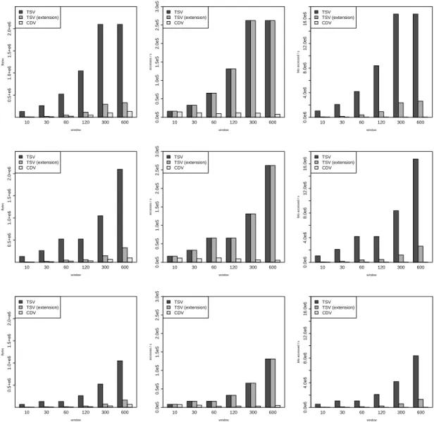
We now examine the cost of the Countdown Vector (CDV) algorithm and compare it to the Timestamp Vector (TSV) algorithm. Figure 5.7 summarizes a diﬀerent set of experiments on our algorithm. To obtain realistic overhead calculations, in this case we run our algorithm on all the three traces already described.

We dimension the vectors for both TSV and CDV appropriate to the observed number of ﬂows in each time window, using [10], bounding the error introduced by the estimation formula to 1%. We dimension our variant of the TSV for a 1 second query frequency. For performance reasons, our implementation restricts the vector sizes to powers of two; we choose the smallest suitable sizes.

Our algorithm has, besides the size of the vector, an additional parameter: the counter initialization value. We have run another round of experiments with various c

values, and have chosen, for each time window, the smallest that obtains at most 0.1% more relative error than the Timestamp Vector algorithm.

Figure 5.7 (left column) shows the high memory savings that our variant of the TSV introduces, at the expense of reducing the query frequency to only one second. In contrast, the CDV we propose further reduces the memory to roughly one half compared to our TSV variant, without introducing such a restriction.

(22)

second, assuming one query every second. We omit the cost of updating the vectors for every packet, since this cost is common to all of the algorithms. It suﬃces to state that, for example, in the nov2007 trace it is only in the order of 50000 accesses per second, which roughly corresponds to the average packet rate in that trace. In Figure 5.7 (central row), it can be observed that the cost of the Timestamp Vector grows with the size of the vector, since it has to be traversed for every query. In contrast, the cost of the Countdown Vector remains small.

This ﬁgure is unfair to our variant of the TSV and to the CDV, since, while the number of memory accesses are equal to those of the original TSV, these are accesses to smaller chunks of memory. Depending on the architecture, then, speciﬁc optimizations could be employed to improve its performance (e.g., read several positions with a single memory access). To correct this, we also present the cost in terms of bits accessed per second in Figure 5.7 (right hand row).

The cost of both variants of the TSV grows proportionally to the vector size, since full vector traversals per query are required. Vectors grow with window sizes, since higher ﬂow counts have to be obtained. In contrast, the CDV’s query cost is constant; in our algorithm, the bulk of the cost is in the maintenance phase. However, since very low counter values can obtain an accuracy very similar to the TSV variants, counter decrements are performed at a low frequency, therefore incurring signiﬁcantly lower costs. These results hold for the three traces we have tested our algorithm on.

(23)

5 10 15 20 0.000 0.005 0.010 0.015 0.020

counter initialization value

relative error 5 10 15 20 0.000 0.005 0.010 0.015 0.020 5 10 15 20 0.000 0.005 0.010 0.015 0.020 5 10 15 20 0.000 0.005 0.010 0.015 0.020 w = 10 s, average error w = 10 s, 95−percentile of error w = 300 s, average error w = 300 s, 95−percentile of error w = 600 s, average error w = 600 s, 95−percentile of error 5 10 15 20 0.000 0.005 0.010 0.015 0.020

relative error 5 10 15 20 0.000 0.005 0.010 0.015 0.020 5 10 15 20 0.000 0.005 0.010 0.015 0.020 5 10 15 20 0.000 0.005 0.010 0.015 0.020 w = 10 s, average error w = 10 s, 95−percentile of error w = 300 s, average error w = 300 s, 95−percentile of error w = 600 s, average error w = 600 s, 95−percentile of error

Figure 5.4: Error of the Countdown Vector algorithm (top) and error of the Count-down Vector algorithm compared to the estimates of the Timestamp Vector algorithm (bottom) using thenov2007 trace.

(24)

5 10 15 20 0.000 0.005 0.010 0.015 0.020

Figure 5.5: Error of the Countdown Vector algorithm (top) and error of the Count-down Vector algorithm compared to the estimates of the Timestamp Vector algorithm (bottom) using theapr2008 trace.

(25)

5 10 15 20 0.000 0.005 0.010 0.015 0.020

Figure 5.6: Error of the Countdown Vector algorithm (top) and error of the Count-down Vector algorithm compared to the estimates of the Timestamp Vector algorithm (bottom) using thenlanr2005 trace.

(26)

10 30 60 120 300 600 window Bytes TSV TSV (extension) CDV 0.5+e6 1.0+e6 1.5+e6 2.0+e6 10 30 60 120 300 600 window accesses / s TSV TSV (extension) CDV 0.0e5 0.5e5 1.0e5 1.5e5 2.0e5 2.5e5 3.0e5 10 30 60 120 300 600 window bits accessed / s TSV TSV (extension) CDV 0.0e6 4.0e6 8.0e6 12.0e6 16.0e6 10 30 60 120 300 600 window Bytes TSV TSV (extension) CDV 0.5+e6 1.0+e6 1.5+e6 2.0+e6 10 30 60 120 300 600 window accesses / s TSV TSV (extension) CDV 0.0e5 0.5e5 1.0e5 1.5e5 2.0e5 2.5e5 3.0e5 10 30 60 120 300 600 window bits accessed / s TSV TSV (extension) CDV 0.0e6 4.0e6 8.0e6 12.0e6 16.0e6 10 30 60 120 300 600 window Bytes TSV TSV (extension) CDV 0.5+e6 1.0+e6 1.5+e6 2.0+e6 10 30 60 120 300 600 window accesses / s TSV TSV (extension) CDV 0.0e5 0.5e5 1.0e5 1.5e5 2.0e5 2.5e5 3.0e5 10 30 60 120 300 600 window bits accessed / s TSV TSV (extension) CDV 0.0e6 4.0e6 8.0e6 12.0e6 16.0e6

Figure 5.7: Memory consumption (left), number of memory accesses per second (center), and number of bits accessed per second (right) for the three algorithms with varying window sizes. Each row corresponds to a diﬀerent trace: the ﬁrst to nov2007, the second to apr2008 and the third tonlanr2005.

(27)

Chapter 6

Conclusions

Implementing a network flow counting algorithm for use in a passive network monitoring system is not trivial, since the hash table based naive algorithm is too slow for the massive data rates associated to network traffic, and, since it requires maintaining one entry per flow, it is impractical for backbone link monitoring.

We have reviewed the available techniques found in the literature, including proba-bilistic linear-time counting. This technique can extract approximate ﬂow counts in a very eﬃcient way using a vector of bits.

Counting ﬂows over sliding windows is even a harder problem, since the inactive ﬂows must be forgotten as they slip out of the window. The literature provides the Times-tamp Vector algorithm, which is a straightforward adaptation of probabilistic linear-time counting. However, this algorithm replaces the vector of bits by a vector of timestamps, which are typically 64 bits long, thus using 64 times as much memory.

Firstly, we have presented a variation of the Timestamp Vector algorithm that, in-stead of operating over continuously advancing sliding windows, it operates over the “discretely advancing” jumping window model. If the window advances in fractions of the window size, the Timestamp Vector can reduce memory requirements the larger the window jumps, the larger the memory savings.

Secondly, we have presented an algorithm called Countdown Vector that calculates the number of ﬂows present in the network traﬃc over sliding windows. Our scheme introduces a continuous maintenance cost but, unlike previous proposals, can be queried in constant time. The basic idea behind our scheme is to use a vector of timeout counters that expires old information in an approximate fashion.

We have performed an evaluation using three real traﬃc traces, and compared the cost in terms of memory and CPU to the state of the art Timestamp Vector algorithm. The Countdown Vector shows comparable accuracy with signiﬁcantly lower costs when compared to both the original Timestamp Vector, and also compared to our extension to the jumping window model.

While in this work we implement the idea of using timeout counters on the direct bitmaps technique, we plan on adapting our scheme to other more eﬃcient ﬂow counting algorithms. In particular, this scheme can be easily applied to the algorithms proposed

(28)

by Estan et al. in [1].

Another important piece of future work is to perform a theoretic analysis of the accuracy of the algorithm we propose. While we have performed an empirical analysis using three representative network traﬃc traces, it is important to be able to provide error bounds that apply to other scenarios.

(29)

Bibliography

[1] Estan, C., Varghese, G., Fisk, M.: Bitmap algorithms for counting active ﬂows on high speed links. In: Proc. of ACM SIGCOMM Internet Measurement Conf. (IMC). (October 2003)

[2] Fusy, E., Giroire, F.: Estimating the number of Active Flows in a Data Stream over a Sliding Window. In: Proceedings of the 4th SIAM Workshop on Analytic Algorithmics and Combinatorics. (2007)

[3] Kim, H., O’Hallaron, D.: Counting network ﬂows in real time. In: Global Telecom-munications Conference, 2003. GLOBECOM’03. IEEE. Volume 7. (2003)

[4] Roesch, M.: Snort–Lightweight Intrusion Detection for Networks. In: Proceedings of USENIX Systems Administration Conference (LISA ’99), Seattle, WA (November 1999)

[5] Paxson, V.: Bro: a system for detecting network intruders in real-time. In: Pro-ceedings of the 7th conference on USENIX Security Symposium, 1998-Volume 7 table of contents, USENIX Association Berkeley, CA, USA (1998) 3–3

[6] Fang, W., Peterson, L.: Inter-AS traﬃc patterns and their implications. In: IEEE Global Communications Conf. (GLOBECOM). (1999)

[7] Cisco Systems: NetFlow services and applications. White Paper (2000)

[8] Barlet-Ros, P., Iannaccone, G., Sanjuàs-Cuxart, J., Amores-López, D., Solé-Pareta, J.: Load shedding in network monitoring applications. In: Proc. of USENIX Annual Technical Conf. (June 2007)

[9] Duﬃeld, N., Lund, C., Thorup, M.: Properties and prediction of ﬂow statistics from sampled packet streams. In: Proc. of ACM SIGCOMM Internet Measurement Workshop (IMW). (November 2002)

[10] Whang, K.Y., Vander-Zanden, B.T., Taylor, H.M.: A linear-time probabilistic counting algorithm for database applications. ACM Trans. Database Syst. 15(2) (June 1990)

[11] Prasad, R., Dovrolis, C., Murray, M., Claﬀy, K.: Bandwidth estimation: metrics, measurement techniques, and tools. Network, IEEE17(6) (2003) 27–35

(30)

[12] : Cisco Systems http://www.cisco.com.

[13] Barlet-Ros, P., Iannaccone, G., Sanjuàs-Cuxart, J., Solé-Pareta, J.: Robust network monitoring in the presence of non-cooperative traffic queries. Computer Networks (October 2008 (in press))

[14] Muthukrishnan, S.: Data Streams: Algorithms And Applications. Now Publishers Inc (2005)

[15] Babcock, B., Babu, S., Datar, M., Motwani, R., Widom, J.: Models and issues in data stream systems. In: Proceedings of the twenty-ﬁrst ACM SIGMOD-SIGACT-SIGART symposium on Principles of database systems, ACM Press New York, NY, USA (2002) 1–16

[16] Hayes, B.: The Britney Spears Problem http://www.americanscientist.org/issues/ pub/the-britney-spears-problem.

[17] Flajolet, P.: Counting by coin tossings. In: ASIAN. Volume 4., Springer (2004) 1–12

[18] Durand, M., Flajolet, P.: Loglog Counting of Large Cardinalities. LECTURE NOTES IN COMPUTER SCIENCE (2003) 605–617

[19] Giroire, F.: Order statistics and estimating cardinalities of massive data sets. In: International Conference on Analysis of Algorithms DMTCS proc. AD. Volume 157. (2005) 166

[20] Metwally, A., Agrawal, D., El Abbadi, A.: Why go logarithmic if we can go linear?: Towards eﬀective distinct counting of search traﬃc. In: Proceedings of the 11th international conference on Extending database technology: Advances in database technology, ACM New York, NY, USA (2008) 618–629

[21] Cohen, E., Strauss, M.: Maintaining time-decaying stream aggregates. In: Pro-ceedings of the twenty-second ACM SIGMOD-SIGACT-SIGART symposium on Principles of database systems, ACM New York, NY, USA (2003) 223–233

[22] Datar, M., Gionis, A., Indyk, P., Motwani, R.: Maintaining stream statistics over sliding windows:(extended abstract). In: Proceedings of the thirteenth annual ACM-SIAM symposium on Discrete algorithms, Society for Industrial and Applied Math-ematics Philadelphia, PA, USA (2002) 635–644

[23] Carter, J.L., Wegman, M.N.: Universal classes of hash functions. J. Comput. Syst. Sci. 18(2) (April 1979)

[24] Jacobson, V., Leres, C., McCanne, S.: libpcap. Lawrence Berkeley Labo-ratory, Berkeley, CA. Initial public release June 1994. Currently available at http://www.tcpdump.org.

(31)

[26] Golab, L., DeHaan, D., Demaine, E., Lopez-Ortiz, A., Munro, J.: Identifying frequent items in sliding windows over on-line packet streams. In: Proceedings of the 3rd ACM SIGCOMM conference on Internet measurement, ACM New York, NY, USA (2003) 173–178