An Effective Model for the Flat Bands of a Dice Lattice

Master Thesis

An Effective Model for the Flat Bands of a

Dice Lattice

Lena Engstr¨

om

Condensed Matter Theory, Department of Theoretical Physics, School of Engineering Sciences

Royal Institute of Technology, SE-106 91 Stockholm, Sweden Stockholm, Sweden 2017

Akademisk avhandling f¨or avl¨aggande av teknologie masterexamen inom ¨amnesomr˚adet teoretisk fysik.

Scientific thesis for the degree of Master of Engineering in the subject area of The-oretical physics.

TRITA–FYS 2017:49 ISSN 0280-316X

ISRN KTH/FYS/–17:49SE c

Lena Engstr¨om August 2017

Abstract

In lattice models with flat (dispersionless) Bloch bands ground state properties will be dominated by interactions between particles. Flat bands possess the property that particles will be localized to a few sites in the lattice. If interactions are added to such a system, particles will only interact with the few neighbouring states with which they overlap. Not only does the localization result in the possibility for exotic phases to emerge, but it also allows for the interactions to be treated through a projection onto the localized states. In this work the, largely unexplored, flat band limit of the dice lattice is introduced and an effective model for the low-energy states of a generic Hubbard-type Hamiltonian is derived. We then specialize to the case of attractively interacting fermions. In addition, we characterize the ground states in the few-particle limit. The effective model includes several interaction terms, on-site and nearest neighbour terms as well as interactions on triangles. Fermion pairs will dominate for an attractive system. The model is mapped onto a ferromagnetic Heisenberg Hamiltonian which is valid for states containing only pairs. Further, a prediction for many-body ground states at any filling of the lattice is made through a perturbative approach. The full ground state for few particles is found to be dominated by pairs uniformly distributed in the lattice. In summary, we here present a simple spin model that is shown to describe the dominating properties arising from an attractive interaction in a flat band.

Key words: flat bands, Dice lattice, 2D lattices, Ultracold gases, Hubbard model, Heisenberg model, effective Hamiltonian, projection

I gittermodeller med platta (dispersionsl¨osa) Bloch band kommer grundtillst˚andets egenskaper att vara dominerade av interaktioner mellan partiklar. Platta band har egenskapen att partiklar kommer att vara lokaliserade till ett f˚atal punkter i gittret. Om interaktioner l¨aggs till i ett s˚adant system, interagerar partiklar bara med de f˚a angr¨ansade tillst˚anden som de ¨overlappar med. Lokalisering resulterar inte bara i m¨ojligheten f¨or exotiska faser att uppst˚a utan det till˚ater ¨aven interaktioner att be-handlas via en projektion till de lokaliserade tillst˚anden. Detta arbete introducerar det, till st¨orsta dels outforskade, t¨arningsformade gittret och h¨arleder en effektiv modell f¨or l˚agenergitillst˚aden f¨or en generisk Hubbardmodell. Vi studerar sedan s¨arskilt fallet med attraktivt interagerande fermioner. Dessutom karakt¨ariserar vi grundtillst˚anden i gr¨ansen med f˚a partiklar. Den effektiva modellen inkluderar flera interaktionstermer, interaktioner p˚a samma punkt i gittret, interaktioner mellan angr¨ansande punkter, och interaktioner i triangelformer. Fermioner som bildar par kommer att dominera i det attraktiva systemet. Modellen avbildas till en ferromag-netisk Heisenberg Hamiltonian, vilken kommer att vara giltig i system som bara inneh˚aller par. Vidare g¨ors en f¨oruts¨agelse om m˚angpartikeltillst˚anden f¨or godtyck-lig fyllning av gittret genom ett perturbativt tillv¨agag˚angss¨att. Det fullst¨andiga grundtillst˚andet f¨or f˚a partiklar domineras av par j¨amnt distribuerade i gittret. Sammanfattningsvis s˚a presenteras h¨ar en enkel spinmodell som visas beskriva de dominerade egenskaperna som uppkommer fr˚an en attraktiv interaktion i ett platt band.

Nyckelord: platta band, t¨arningsformat gitter, 2D gitter, ultrakalla gaser, Hub-bard modellen, Heisenberg modellen, effektiv Hamiltonian, projektion

Acknowledgements

I would like to express my gratitude to my supervisor Professor Sebastian Huber at ETH Z¨urich for giving me the opportunity to do this project. With his valuable insights and experience in the field his guidance steered the work into its best possible version. I owe him many thanks for the introduction into this exciting field of physics.

I would also like to thank Murad Tovmasyan for his guidance and help, with-out which I would have been quite lost. He has invested his time and full effort throughout this project, by making himself available for discussions and providing a sound theoretical background.

I also extend a thank you to my examiner at KTH, Professor Jack Lidmar, for all the information provided and the help with the formalities concerning the thesis.

Contents

2.2 Band structure without magnetic field . . . 5

2.3 Aharonov-Bohm Cages . . . 6

2.3.1 Magnetic Translational Operator . . . 8

2.3.2 Band structure . . . 8

2.3.3 Bloch states . . . 11

2.3.4 Chern numbers for bands . . . 12

2.4 Wannier Functions . . . 13

2.4.1 Maximally Localized in Marzari-Vanderbilt sense . . . 13

2.4.2 Localized states . . . 14

2.5 Conclusion . . . 18

3 Projecting the interaction 19 3.1 Effective lattice . . . 20 3.2 Bosons . . . 22 3.3 Fermions . . . 25 3.4 Conclusion . . . 26 4 Spin Mapping 29 4.1 Heisenberg model . . . 31 4.2 Chemical potential . . . 32 4.3 Conclusion . . . 32 vii

5 Few-particle problem 35

5.1 Two-particle problem . . . 37

5.1.1 Corresponding spin state . . . 39

5.2 Two-pair problem . . . 40

5.3 Exact Diagonalization . . . 43

5.4 Second order perturbation of the ground state . . . 44

5.4.1 General eigenstate with a split-up pair . . . 45

5.5 Towards the many-body problem . . . 48

6 Conclusion and outlook 51

A Projection Bosons 53

B Projection Fermions 59

C Spin mapping 63

D Calculations eigenstates 65

Chapter 1

Introduction

Lattice models with completely flat Bloch bands offer systems where interacting ground state properties can be studied in detail. In a flat bands all particles will have a vanishing group velocityv=∂E_∂k = 0. That is to say that the eigenstates are immobile and do not contribute to the transport properties of the system. Particles are then localized to a limited number of sites in the lattice. This localization is however a single particle effect. Interactions between particles will instead domi-nate the properties and transport becomes possible through the interaction effects. To characterize these properties the goal is to study how particles interact on such flat bands. Interacting particles do not have well-defined separable single particle states since a particle affects the states of the other particles. The interaction ef-fects can for the flat bands be characterized with methods otherwise unavailable. Since the non-interacting states are localized in the flat band an effective model can be given for low energies. This thesis makes predictions for the low-energy states of the dice lattice by projecting interactions onto the lowest flat band. The model and lattice that describe the dominant processes can then be greatly simplified. The dice lattice, also called the T3 lattice, is in this thesis studied for a tight binding model. The non-interacting model consists of three bands which under a magnetic field, with a specific value, can become separated and flat. The flatness of the bands arises from frustration in the hopping elements. Frustrated hopping is an interference effect where classical paths for the particles interfere destructively due to the geometric frustration. Eigenstates in this model will then be restricted to a limited number of sites. Other bipartite lattices of the same class, such as the Kagome lattice, the Lieb lattice, and the Creutz ladder, similarly result in frus-trated hopping [1–6]. Generally in hopping problems the low energy physics is well described by the long-wavelength part of the dispersion relation. However, due to the flatness of the bands the states will behave quite differently here.

The effect of an on-site Hubbard interactionU is studied by projecting the inter-action onto the localized eigenstates of the non-interacting model. The projection results in an low-energy effective model with a larger number of interaction terms. The interaction constantU can be chosen to be either repulsiveU >0 or attractive U <0. The model for hard-core bosons with a repulsive interaction has been stud-ied for the dice lattice [7–10] and results in a supersolid at low filling. The fermionic model is here studied further. For an attractive interaction the formation of pairs will be beneficial. However, since there are terms that break pairs the effect from these terms on the full state must be evaluated.

The two following chapters derive the effective model starting with a simple tight binding model. In chapter 2 the properties of the dice lattice is calculated, by find-ing the band structure and the localized eigenstates. In chapter 3 the interaction is projected for both bosons and fermions. In the two next chapters the full effective model is evaluated to find the low-energy ground state for low fillings. In chapter 4 the pair-breaking terms are removed. Under the assumption that the model only contains pairs the Hamiltonian can be mapped onto a spin-1/2 Heisenberg model. In chapter 5 the ground state of the Hamiltonian for low filling is evaluated by studying the two-particle and two-pair problem by splitting the Hamiltonian in two parts. The ground state of the non-perturbed Hamiltonian is found and the possible corrections from second order perturbation theory are approximated. As a conclusion, we will see that due to the small size of the perturbation the simple spin model can be considered to describe the main contributions to the many-body ground state at arbitrary filling.

Chapter 2

Dice Lattice

In this chapter the non-interacting tight binding model for the dice lattice will be solved analytically. Both the bosonic and fermionic case will be considered. All three bands of the model will be seen to become flat and separated when a specific magnetic field is applied. Firstly, the energy bands for the lattice without any ap-plied magnetic field are calculated. Secondly, hopping amplitudes are engineered in such a way that half a magnetic flux unit passes through each rhombus in the lattice for a chosen gauge. This gauge will be chosen so that all hopping amplitudes have a real value. The eigenstates will be given as Bloch states that are transformed into Wannier functions in real space. Finally, these Wannier functions are seen to describe eigenstates that are localized to a few sites in the lattice, i.e. have compact support.

2.1

The tight-binding model

The tight binding model describe single particles that can occupy sites in the lattice and that can hop to a neighbouring site with a hopping amplitudet [11]. These amplitudes can vary depending on what bond a particle hops over and is more generally given asti,j for the bondi, j. For bosons the tight binding Hamiltonian with nearest neighbour hopping is:

ˆ H=−X hi,ji ti,jˆb†iˆbj+t∗i,jˆb † jˆbi =−X hi,ji ti,jˆb†iˆbj+ h.c. , (2.1)

where the annihilation operator ˆbj annihilates a particle at sitej and the creation operator ˆb†_i creates a particle at site i. The bosonic operators are defined by the

commutation relations:

h

ˆ

bi,ˆb†_ji= ˆbiˆb†_j−ˆb†_jˆbi=δi,j, hˆbi,ˆbji= 0, hˆb†_i,ˆb†_ji= 0, (2.2) where:

δi,j

(

1, i=j

0, i6=j . (2.3)

In this number basis, where the states are described by the particle occupation ni at each site, the states are described as operators acting on a vacuum state to create a configuration of particles. If the hopping amplitudet is real and has the same value along any bond in the lattice the Hamiltonian can be simplified to:

ˆ H=−tX hi,ji ˆ b†_iˆbj+ h.c.. (2.4) For fermions the Hamiltonian includes fermionic operators with an additional spin-componentσ. The fermionic operators are defined from the anticommutation rela-tions: n ˆ ci,σ,ˆc†_j,σ0 o = ˆci,σcˆ†_j,σ0+ ˆc †

j,σ0ˆci,σ=δi,jδσ,σ0, {ci,σ,ˆ cj,σˆ 0}= 0,

n ˆ c†_i,σ,ˆc†_j,σ0 o = 0. (2.5) The fermionic Hamiltonian then becomes:

ˆ H=−X hi,ji tσ_i,jˆc†_i,σcˆj,σ+ h.c. . (2.6)

To preserve time-reversal symmetry it is required that the hopping amplitudes for opposite spins are each others complex conjugates tσ_i,j0 =t_i,jσ ∗, where σ =−σ0. The resulting band structure of the model will depend on the geometric structure of the lattice. The number of bands is given by how many sites are included in a unit cell for these to form a Bravais lattice. The shape of the bands and the gap separating them will depend on the unit vectors for the lattice. In each unit cell j there will be one site which belongs to the sublattice m. There are then operators for each sublattice in each unit cell ˆcj,m,σ. The hopping occurs both

between sublattices and between unit cells. Without any further interaction this model can be solved by a Fourier transform of the Hamiltonian since the hopping will be diagonal in the reciprocalk-space. The Fourier transform of the operators takes the form:

ˆ c†_j,m,σ = √1 N X k∈B.Z. e−ik·jcˆ†_k,m,σ, ˆcj,m,σ = 1 √ N X k∈B.Z. eik·jcˆk,m,σ. (2.7)

From here on the fermionic operators will be used for all non-interacting states. The corresponding bosonic operators will differ to the fermionic by the commutation re-lations, where the bosonic commute and the fermionic anticommute, according to

2.2. Band structure without magnetic field 5

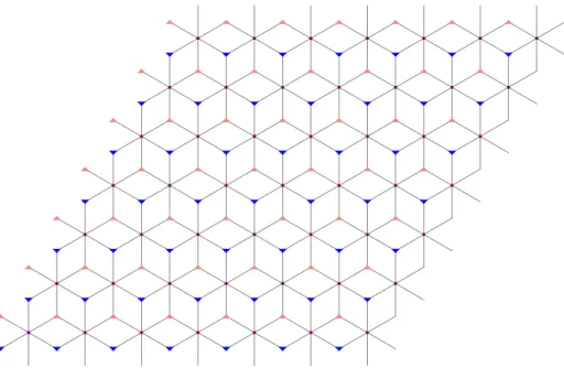
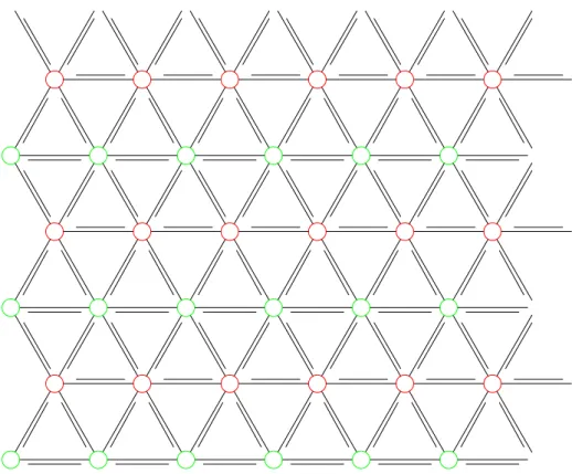
Figure 2.1: The dice lattice. There are two different types of sites, sixfold coordi-nated (circles) and threefold coordicoordi-nated (triangles).

equations (2.2) and (2.5). An arbitrary number of bosons can occupy a site in the lattice, while the Pauli principle restricts the fermions to only allowing occupa-tion of one up-spin and one down-spin fermion at each site. From the tight-binding Hamiltonian the eigenstatesψwill be given by the Schr¨odinger equation ˆHψ=Eψ. In this thesis the dice lattice is considered. The dice lattice is a two dimensional lattice which has three sites in the unit cell and therefore three bands in the non-interacting tight binding model. However, once a magnetic field is added the band structure will change as the field modifies the structure of hopping amplitudes in the lattice.

2.2

Band structure without magnetic field

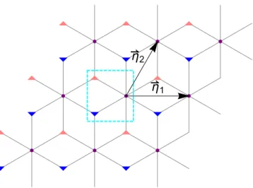
The dice lattice can be seen in figure 2.1. The lattice constanta is given by the length of the link between two neighbouring sites. In the unit cell of the dice lattice three sites are included: one with sixfold coordination (∗) and two with threefold coordination (∆). The unit vectors connect the unit cell from the sixfold coordinated site to another of the same type in the neighbouring unit cells, and are given as:

( η1= √ 3a(1,0) η2= √ 3a1₂, √ 3 2 . (2.8)

In figure 2.2 the unit cell is marked out along with its unit vectors. The unit cells are located on an underlying triangular Bravais lattice.

The band structure of a simple hopping Hamiltonian in the dice lattice is given by the Schr¨odinger equation for the three sites in the unit cell. The eigenvalues of the Hamiltonian are then given by the three bands:

(

0(k) = 0

±(k) =±

√

2p3 + 2 cos (k1) + 2 cos (k2) + 2 cos (k3),

(2.9) where      k1=k·η1 k2=k·η2 k3=k·(η2−η1) (2.10)

are the reciprocal unit vectors and a vector that combines these.

The dice lattice is a bipartite lattice, meaning that the sites can be divided into two disjoint sublattices. For this lattice these are the sixfold and threefold connected sites. The sixfold connected sites only have bonds to threefold connected sites and the other way around. Completely flat bands are achieved by adding a magnetic field perpendicular to the lattice at the right value to form Aharonov-Bohm cages that the particles are localized in [12]. Compared to the= 0 band, that is flat for the lattice without any magnetic field, there is no band touching when all bands are flat. For the separated flat bands it is possible to study localized states in only that band. For bipartite lattices the flat bands contain well localized states [13].

2.3

Aharonov-Bohm Cages

If an external magnetic field is applied the Hamiltonian will be affected by the vector potentialA, connected to the magnetic field asB=∇ ×A:

H = i~ 2m∗∇+V → 1 2m∗(i~∇ −eA) 2 +V. (2.11)

On the form of a tight binding Hamiltonian this means that the hopping amplitude t is affected by the field [12]. Peierls’ substitution is derived from the shifted Hamiltonian. The substitution adds a phase to the hopping amplitude:

t→te−i~e

R

2.3. Aharonov-Bohm Cages 7

η



η



Figure 2.2: Unit cell of the dice lattice with unit vectors.

Where Φ0 =~/e is the unit flux. This means that a particle picks up a phase as

it hops over a bond. For a homogeneous magnetic field the flux over a plaquette is set to a fixed quantity and is given by [14]:

Φ =

I

cell

A·dr= 2πν. (2.13)

To get a system of flat bands the valueν = 1/2 is chosen, so that a flux of Φ =π passes through each plaquette [15, 16]. The hopping amplitudes of the lattices are then to be modified so that a particle picks up a phaseπfrom hopping along the bonds surrounding one elementary rhombus of the dice lattice.

The physical system is gauge invariant since the vector potential results in the same magnetic field B even after a gauge transformation A → A+∇f. The phases can then be chosen in any way as long asπ-flux passes through each plaque-tte. A real gauge can be chosen so that all Aharonov-Bohm phases result in real hopping amplitudes. Theν = 1/2 flux can be achieved in the dice lattice by adding the phase±π for one bond on each elementary rhombus. The hopping amplitude on that bond then shifts fromt→e±iπt=−t. The chosen gauge is shown in figure 2.3 where the bonds with negative hopping amplitude are denoted by a line added on that bond.

Since all the hopping amplitudes have a real value, time reversal symmetry will be preserved by takingtσ0 _{= [t}σ_]∗_{=t, the same amplitude for all spins. With these} modified hopping amplitudes a new unit cell must be chosen, since the translational symmetry of the lattice has been broken.

2.3.1

Magnetic Translational Operator

For the zero-field case the lattice translation operators ˆT_i0commute with the Hamil-tonian and with each other ashTˆ0

1,Tˆ20

i

= 0. The operators are defined as: ˆ T₁0=X m,n ˆ_b† m+1,nˆbm,n Tˆ20= X m,n ˆ_b† m,n+1ˆbm,n. (2.14) However, when an external magnetic field is added the translational symmetry of the lattice is broken and the operators are shifted into new magnetic translation operators [14]: ˆ T₁M =X m,n ˆ b†_m+1,nˆbm,neiθ1m,n _TˆM 2 = X m,n ˆ b†_m,n+1ˆbm,neiθ2m,n_{. (2.15)}

The requirements for these are that they should commute with the Hamiltonian, that has modified hopping amplitudes, and with each other. The operators should then be constructed so that they enclose a super-cell of dimensionk×l on which an integer multiple of the flux 2π is enclosed. To fulfil the requirements of the operators the condition for this super-cell is:

e−iklΦTˆ1M k ˆ T2M l =Tˆ1M l ˆ T2M k . (2.16)

The smallest possible super-cell is the magnetic unit cell, which is given bykl= 1/ν, where ν is given by equation (2.13). For the case whenν = 1/2 this means that the magnetic unit cell has twice as large area as the unit cell for the zero-field case. The new unit cell that has been chosen can be seen in figure 2.3. The unit cell now includes six sites: two sixfold coordinated sites and four threefold coordinated sites. For this gauge choice and unit cell the C3 symmetry of the lattice has been broken, so the unit cells are now placed on an underlying rectangular lattice. The band structure will now be seen to be flat for this model.

2.3.2

Band structure

After adding a flux ofπ through each plaquette the unit cell will consist of twice as many sites. There are now six sites in each unit cell and six bands are expected to arise from the hopping Hamiltonian. As will be seen these are three doubly degenerate energy levels. For this specific value of the flux all of these bands will be flat. The Hamiltonian matrix is given from writing the Schr¨odinger equation on matrix form:

H(k)ψ=Eψ, (2.17)

where the solution is then a vector of the operators for each site in the unit cell

2.3. Aharonov-Bohm Cages 9

1

2

3

4

5

6

Figure 2.3: Unit cell of dice lattice withπ-flux passing through each rhombus. The unit cell contains 6 sites which are numbered.

The eigenvalues and eigenstates of the tight binding Hamiltonian are given by the matrix for the hopping in and between the new unit cells (wheret=−1):

H(k) = =         0 1−e−ik·ex _{1 +e}−ik·ex _{0 1 e}ik·ey 1−eik·ex _{0 0 e}ik·ey _{0 0} 1 +eik·ex _{0 0 −1 0 0} 0 e−ik·ey −_{1 0 1 +e}ik·ex −_{1 +e}ik·ex 1 0 0 1 +e−ik·ex _{0 0} e−ik·ey _{0 0 −1 +e}−ik·ex _{0 0}         , (2.18) where ( ex= √ 3a(1,0) ey= √ 3a 0,√3 (2.19)

are the unit vectors for the new unit cells. These reach from a sites with a specific number to the corresponding sites in neighbouring unit cells. The Brilloiun zone constructed from new reciprocal lattice vectors, is given from the condition:

Ki·ej= 2πδij. (2.20)

The reciprocal unit vectors are:

(

Kx= √2₃π_a(1,0)

Ky =23πa(0,1).

(2.21)

The first Brillouin zone is then given by: kx∈[−_√π

3a, π √ 3a) andky∈[− π 3a, π 3a). The eigenvalues of the Hamiltonian matrix can be found by constructing the following vectors ei = (n1, . . . , ni, . . . , nN)T where ni = 1 and nj = 0 for j 6= i. If the

matrixH(k) now acts twice on the vectorse1 ande4, it can be seen that these are

eigenvectors to theH(k)2_matrix:

H(k)2e1= 6e1 H(k)2e4= 6e4. (2.22)

Two doubly degenerate eigenvalues to the Hamiltonian are=±√6, as the eigen-values ofH(k)2 should be given by2 = 6. A third doubly degenerate eigenvalue is found for= 0. All diagonal elements ofH(k) are 0 meaning that the sum of all eigenvalues must be 0. For theH(k)-matrix the following three doubly degenerate eigenvalues are then found:

(

0(k) = 0

±(k) =±

√

6. (2.23)

The model then has a band gap of ∆ =√6, from each doubly degenerate band to the next. Notably, ∆ is also the bandgap from the lowest band to the next. Models

2.3. Aharonov-Bohm Cages 11

only considering the lowest energy states should be considered for energies below this energy gap as not to include intraband effects. For each degenerate band two eigenstates will be found.

2.3.3

Bloch states

The eigenvectors in the lowest band (=−√6) can be found by constructing them as: |v1i=√1 2 _H(k) √ 6 −I |e1i, |v2i= √1 2 _H(k) √ 6 −I |e4i, (2.24) which written in operators is:

|v1i= h−_√1 2, 1−eik·ex √ 12 , 1+eik·ex √ 12 ,0, 1 √ 12, e−ik·ey √ 12 i ˆ ck |v2i= h0,ei√k·ey 12 ,− 1 √ 12,− 1 √ 2, 1+e−ik·ex √ 12 , −1+e−ik·ex √ 12 i ˆ ck, (2.25)

wherecˆk = [ˆck,1,ˆck,2,ˆck,3,cˆk,4,ˆck,5,cˆk,6] is a vector of the operators for each site

in a unit cell. There will be two eigenvectors for the each eigenvalue since the band is doubly degenerate.

Similarly to the lower band the eigenstates for the upper band ( = √6) can be constructed as: |u1i=√1 2 _H(k) √ 6 +I |e1i, |u2i=√1 2 _H(k) √ 6 +I |e4i, (2.26) which is: |u1i= h√1 2, 1−eik·ex √ 12 , 1+eik·ex √ 12 ,0, 1 √ 12, e−ik·ey √ 12 i ˆ ck |u2i= h0,eik·ey √ 12 ,− 1 √ 12, 1 √ 2, 1+e−ik·ex √ 12 , −1+e−ik·ex √ 12 i ˆ ck. (2.27)

The eigenstates to the zero band are not as straight forward to find as for the other bands. Consider the projectors of each band that projects any state onto the band: P−=|v1ihv1|+|v2ihv2|, P+ =|u1ihu1|+|u2ihu2|, P0=|z1ihz1|+|z2ihz2|.

(2.28) All the bands should span the total Hilbert space of the system. The projectors into the subspace of each band should then have the completeness relation:

P++P−+P0=I. (2.29)

This condition will be fulfilled for the following Bloch states:

|z1i= √ 1 18−12 cos (k·ex) 0,−2isin (k·ex)−eik·ey_{,2 cos (k·ex)−3,0,0,} 1−e−ik·ex_+e−ik·ey _+e−i(k·ex+k·ey) ˆ ck |z2i= √ 1 18−12 cos (k·ex) 0,1−eik·ex_+eik·ey_+ei(k·ex+k·ey)_,0,0, 2 cos (k·ex)−3,−2isin (k·ex) +e−ik·ey ˆ ck. (2.30)

When these are multiplied by the matrix of the Hamiltonian the eigenvalue is 0.

2.3.4

Chern numbers for bands

The Chern number C is a topologically invariant quantity that is defined for an isolated band s. The topological invariance means that the system cannot adia-batically be transformed into a system with a different Chern number. The Chern number is for that reason often used as a topological index for the band. It has been proven that for the three properties in tight binding models: a flat band, a non-zero Chern number, and local hopping, all cannot be fulfilled at once [17]. The dice lattice model already has two of these properties, nearest neighbour hopping and flat bands. The Chern number is then expected to vanish. The Chern num-ber is a property derived from the Berry phase. The Berry phase describes the phase that a state picks up in parameter space during its time evolution. As the Bloch states are defined in the reciprocal k-space, the Berry phase describes the phase picked up in the Brillouin zone [18]. The Berry connection (which is gauge dependent) is the vector potential for the Berry phase and is given by:

Asβ(k) =−ihus(k)|∂kβ|u

s_{(k)i, (2.31)}

where kβ is one of the directions in k-space and |us(k)iare the Bloch functions. The Berry curvature (which is gauge independent) is given by:

F_αβs (k) =∂kαA

s

β(k)−∂kβA

s

α(k). (2.32)

The Chern number is then an intrinsic property of the band structure and is given by: Cs₌ 1 4π2 Z B.Z. F₁₂s(k)d2k, (2.33) whereCs_{is an integer number. For the lower bands the Berry connection will be a} constant, resulting in thatF₁₂−,1(k) = 0 and a zero Chern numberC−,1_{= 0. Since}

the other Bloch state in the lower bands consists of the same weights but rearranged this will also result in a zero Chern numberC−,2_{= 0. For the upper band the Chern}

number will, by the same argument, be zero as well: C+,1_=C+,2_{= 0. For the zero}

bands the Berry curvature have a non-zero value. However, the Chern number will still be C0,1 _{= 0. For the other Bloch state in the zero bands we get the same}

results, withC0,2 _{= 0. However, the Berry curvature appears with a minus sign,}

F₁₂0,2(k) =−F₁₂0,1(k). Since the Chern number is zero for all bands these are trivial Chern bands.

2.4. Wannier Functions 13

2.4

Wannier Functions

The eigenfunctions to the dice lattice that have been considered so far have been Bloch states in the reciprocalk-space. These states can be expressed in real space via Wannier functions [19]. The Wannier function for a bandnis constructed as:

|Rni= L d (2π)d Z B. Z. ddke−ik·R|ψnki, (2.34)

where |ψnki is a Bloch state. The spread of the Wannier function is smaller for

a larger spread in k-space and vice versa. Generally, Wannier functions are not eigenstates to a band since they have contributions from allk-states. Only in a flat band, where allk-values give the same energy, can Wannier functions constructed from the Bloch states be corresponding eigenstates. The Wannier functions are centered at a home cellR= 0. However, due to the periodicity of the lattice the entire function can be shifted by the lattice translation operator. The spread of the Wannier function therefore determines the overlap between Wannier functions at different sites. Generally, Wannier functions are not expected to be compact in space. However, for a flat band localized states are expected to exist. There then exists Wannier function that extend only to a limited number of sites. Having compact Wannier functions is a helpful property that can be used to express states in real space. Procedures that generally cannot be used, that utilizes the properties of Wannier functions as eigenfunctions, are then possible in flat bands. When con-sidering effective models for the localized states the overlap between states are the only sites where interactions can occur. If the Wannier functions only extend to a few finite number of states the model can be projected onto those states exactly, without the need of truncation.

There exists a gauge freedom in Bloch functions where a phase can be inserted while the function remains an eigenstate. However, in the Fourier transform in equation (2.34) a shift of the phase will result in a different Wannier function. There then exists some gauge for the Bloch function that results in the minimized spread of the Wannier function.

The Wannier functions for the states in the lowest band will be given by:

|R,−,1i= ₍₂N_π)2 R B. Z.d 2_{k e}−ik·R _|v1i |R,−,2i= ₍₂N_π)2 R B. Z.d 2_{k e}−ik·R _|v2i. (2.35)

2.4.1

Maximally Localized in Marzari-Vanderbilt sense

Wannier functions are defined up to a gauge choice. Depending on what gauge they are calculated for the spread of the function in real space will vary. The gauge of a single band can be changed by modifying the Bloch states with a phase:

For all Bloch states there exists one preferred gauge that results in the maximal localization of the Wannier state. Due to the band degeneracy in the model methods for composite bands can be applied to find the maximally localized states [20]. Bloch states within the same degenerate band can by a unitary transformation result in new Bloch states:

|ψn˜ ki=

X

m

U_nm(k)|ψmki. (2.37)

The smoother the gauge the more localized the Wannier states are in real space. For the Bloch states from equations (2.25) and (2.27), the Wannier states for the upper and lower band are localized to a finite number of sites. In figure 2.4,|ψ(r)|2

for the Wannier functions in the lowest band is plotted for each site in the lattice. In only three unit cells (for each state) weights have a non-zero value. As these states are strictly localized they are already in the gauge leading to maximal localization. For the zero band the Wannier functions retrieved from equation (2.30) are strictly localized in one direction and exponentially localized in the other. The two Wan-nier functions for this band can be seen in figure 2.5. The localized states can also be found using the recursion method from [16]. The localized states for the upper and lower bands are found for the weights that result in a destructive interference outside the state when a sixfold coordinated site is at the center. Strictly localized states can in the same way be found for the zero bands by setting the threefold coordinated site as the center of the states. The states in the zero band will however not be orthogonal to each other.

2.4.2

Localized states

For the lowest band two strictly localized states can be chosen. These are ”flower”-shaped states which come in two types and are localized to seven sites each. The largest weight is centered at the sixfold coordinated sites of a unit cell and each is surrounded by six weights at the surrounding neighbouring sites. These states can be seen in figure 2.6 where the distribution of weight is given by the Wannier function (as seen in figure 2.4). For the upper band the localized state are given by a change of the sign for the middle weights. The upper band is denoted by (+) and the lower band by (−). The eigenstates for the zero band will however have a different form. The localized states for the upper and lower band are explicitly given in the real space operators as:

|∗±₁i=√1 12 h ±√6ˆb†_j,1+ ˆb†_j,2+ ˆb†_j,3+ ˆb†_j,5−ˆb†_j+ex,2+ ˆb†_j+ex,3+ ˆb†_j−ey,6i|0i (2.38) |∗±₂i=√1 12 h ±√6ˆb†_j,4+ ˆb†_j,5−ˆb†_j,6−ˆb†_j,3+ ˆb†_j−e x,5+ ˆb † j−ex,6+ ˆb † j+ey,2 i |0i (2.39) where the vectorsex andey are the unit vectors to the next extended unit cell in thex- or y-direction. They are here given on bosonic form for the operators ˆbj,i

2.4. Wannier Functions 15

Figure 2.4: Weights of the Wannier functions of|v1i and|v2i, (eigenstates of the lower band), where the area of each filled circle is proportional to the weight at each site. There exists 2 types of states, one centered at site 1 of the unit cell (green) and the other centered at site 4 (red). The weights at the centered sites have the value 1₂ and the weights at the surrounding sites are ₁₂1. Sites where the coefficient of the wavefunction has a negative sign are marked with a darker color.

Figure 2.5: Weights of the Wannier functions of|z1i and|z2i, (eigenstates of the

zero band), where the area of each filled circle is proportional to the weight at each site. There exists 2 types of states, one centered at site 3 of the unit cell (green) and the other centered at site 5 (red). The weights at the centered sites have the value 0.017. Sites where the coefficient of the wavefunction has a negative sign are marked with a darker color.

2.4. Wannier Functions 17

Figure 2.6: The two types of localized ”flower” states in the upper and lower bands that span the degenerate bands. The rim sites with stripes have a coefficent with a negative value.

which acts upon sitei in unit cellj.

The states can be seen to be orthonormal to states centered at different sites, both for those of the same type of state and for the other type. In figure 2.7 it can be seen how the states can be placed to span the entire lattice. The figure also includes all configurations in which states can overlap. States further than neighbouring states share no sites where both have weights and the overlap is there 0. For states that are neighbouring two sites are always shared. The overlap will however be equal in size but with opposite sign resulting in an overlap of 0. Further, for the threefold coordinated sites a maximum of three states can overlap at once.

Figure 2.7: Orthogonal localized states in the lower band. The states form a triangular effective lattice.

2.5

Conclusion

A dice lattice with a magnetic flux has been considered and the eigenstates of the tight binding Hamiltonian have been found as Bloch states. The maximally localized Wannier functions have been found for the two eigenstates that are an orthogonal basis for the lowest band. These are two types of strictly localized states in real space that have non-zero weights only at seven sites each. Moreover, since there is no hopping taking place outside of these states there is also no transport through the lattice. To study the interaction between particles the hopping can be ignored for an effective model that instead projects the interaction so that it acts between localized states. In the following chapter the exact projection, between particles at sites in the lattice and localized states in the lowest band of the lattice, is utilized to get an effective Hamiltonian.

Chapter 3

Projecting the interaction

The localized states and flat bands described in the previous chapter are single particle properties of the dice lattice. For the non-interacting case an arbitrary filling of the lattice, states are given as product states of single particle states, which will be symmetrized or antisymmetrized for the bosonic or fermionic case respectively. If an on-site interaction is added the model can no longer be solved exactly via a Fourier transform and other analytical tools must be used to describe the properties of the resulting systems [21]. Numerical solutions are also not trivial for solving the problem at arbitrary filling, but require large computational power. In this and the following chapters the interaction problem will be approached by formulating a model giving explicitly the effective interaction for the specific states of interest. To get an effective model for the low energy states of the interacting system a projection into a part of the Hilbert space can be made. The full model is in this chapter projected onto the localized states of the lowest band. However, to assure that the interaction keeps particles in the lower band the interactionU must be lower than the bandgap to the next band ∆: U ∆. This condition assures that the lowest states remain in the lowest single particle energy band. Due to the strictly localized states of the lower band a mapping onto these will be exact under these conditions.

The model that we consider is a Hubbard model ˆH = ˆHkin + ˆHint, where the

interaction is an on-site density interaction. The on-site Hubbard interaction can then be studied by considering what the effect of the interaction is on the local-ized states. That is to say, the effective model is derived via a projection onto the lowest band. The full fermionic operator can be considered to be a combination of operators that act on a single band:

ˆ ci,σ = X j [ ˆW−(i−j)]∗ˆvj,σ+ X j [ ˆW0(i−j)]∗zˆj,σ+ X j [ ˆW+(i−j)]∗uˆj,σ, (3.1) 19

where ˆvj,σ is an operator for the site j in a state in the lower bands, ˆzj,σ is an operator for states in the zero bands, and ˆuj,σ is an operator for states in the upper bands. The coefficients ˆWs_{(i−j), for a band s, are those given by the Wannier} function of a state centered at site iin that band. An operator ¯ci,σ that acts on an entire localized state in the lower band can then be defined by projecting the operators at single sites via the Wannier function for the states. The projection acts as: ¯ ci,σ = X j [ ˆW−(i−j)]∗ˆvj,σ ¯c†i,σ = X j ˆ W−(i−j)ˆv_j†_,σ. (3.2) The projection that instead goes to the single site operator from the flat band operators, is then given by:

ˆ vj,σ = X i ˆ W−(i−j)¯ci,σ ˆv†j,σ = X i h ˆ W−(i−j)i ∗ ¯ c†_i,σ. (3.3) The projection onto the lower band is to project the model onto only a part of the Hilbert space. The projection can similarly be done for the rest of the Hilbert space, the two other degenerate bands. The resulting complementary operator ˜ci,σ then gives the full model together with the flat band operator. From equation (3.1):

ˆ

ci,σ = ¯ci,σ+ ˜ci,σ, (3.4) where the projection onto the rest of the Hilbert space is given by:

˜ ci,σ= X j [ ˆW0(i−j)]∗zˆj,σ+ X j [ ˆW+(i−j)]∗uˆj,σ. (3.5) The projections for the fermionic and the bosonic cases will differ due to both that the Hamiltonians will be different and that the statistics of the operators are different.

3.1

Effective lattice

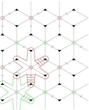
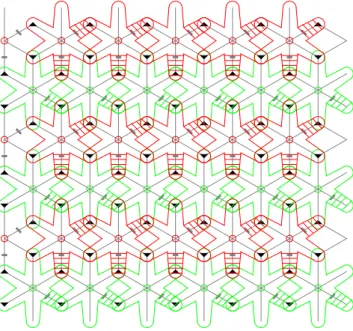
The new effective lattice that the effective Hamiltonian acts on is a triangular lattice, see figure 3.1. There are two types of non-equivalent sites due to the two types of Wannier functions spanning the degenerate lowest band. The sites of the triangular lattice are the centered sites of each localized ”flower” state. The matrix elementsσii_jk = ±1 appear for the bond jk, on the side with the triangle containingi, as a double line to indicate a negative sign. This matrix element only affects the processes on the triangles in the effective Hamiltonian given after the projection, equation (3.13) (fermions) or equation (3.9) (bosons). The other types of interaction terms remain unaffected by the signs of the bonds and instead act on an ordinary triangular lattice. The unit vectors of the triangular lattice are the same as the unit vectors for the original dice lattice (see equation (2.8)).

3.1. Effective lattice 21

Figure 3.1: The effective triangular lattice of the lower band when the interaction has been projected onto the two types of localized ”flower”-states. The double lines mean that the intetaction sign for that triangle has a negative signσii_jk=−1, when the triangle consists of the cornersi, j, k. These signs are only valid for the interactions concerning three sites. The sign of the interaction only depends on the double lines inside of the triangle. The double line are then only valid for one side of the bond.

3.2

Bosons

In the Bose-Hubbard model the on-site interaction takes the form:

ˆ Hint= U 2 X i ˆ ni(ˆni−1) = U 2 X i ˆ_b† iˆb † iˆbiˆbi, (3.6)

where an interactionU/2 arises when more than one boson occupies a site i. If there are no restrictions to how many bosons that can occupy the same site the energy from having two bosons at the same site isU, having three bosons is 3U, and so on. The on-site interaction can be projected onto the flat band by using equation (3.3) to write the bosonic operators for the full model ˆbi,σ in the operators for the localized states in the lower band ¯bi,σ. If these operators are inserted into

the interaction, coefficients for each projected term are given by:

Vijkl= U∆ X µ∈∆ [ ˆW−(i−µ)]∗[ ˆW−(j−µ)]∗Wˆ−(k−µ) ˆW−(l−µ) + U∗ X n∈∗ [ ˆW−(i−n)]∗[ ˆW−(j−n)]∗Wˆ−(k−n) ˆW−(l−n), (3.7)

where Greek indices indicates the threefold connected sites and Latin indices indi-cates sixfold connected sites. With these indices the projected Hamiltonian is given as all combination of overlaps by summing over all possible combination of sites, for the projected operators:

¯ Hint= 1 2 X i,j,k,l Vijkl¯b†i¯b † j¯bk¯bl. (3.8)

It can be seen directly from the localized ”flower” states that most of these terms will be 0. The only non-zero overlap between localized states (in the lower band) occurs with only one, two, or three neighbouring states at once. In the real gauge all weights are real so that [ ˆW−(j−µ)]∗= [ ˆW−(j−µ)] and ˆW_↓−(j−µ) = ˆW_↑−(j−µ). The overlap of states can be non-zero only at µ- or n-sites where a maximum of three localized states are centered at neighbouring n-sites. The indices i, j, k, l can be combined to get all combinations of contributing states in the projection. The possible combinations will be those where all indices are the same, where three are the same, and where two are the same. The calculation for the contributions

¯

3.2. Bosons 23 becomes: ¯ Hint= γ1 X i ¯ ni(¯ni−1) +4γ2 X hi,ji ¯ nin¯j +γ2 X hi,ji h ¯ b†_i2¯b2_j+ h.c.i +4γ3 X ∆(i,j,k) σii_jkhn¯i¯b†j¯bk+ h.c. i +2γ3 X ∆(i,j,k) σii_jkh¯b†_i2¯bj¯bk+ h.c. i , (3.9) where γ1 = _U ∗ 8 + U∆ 48 , γ2 = U∆ 144 and γ3 = U∆

288. Here hi,ji is a sum over all pairs of nearest neighbours. The effective lattice on which these interactions act is the triangular lattice in figure 3.1. The sum ∆(i,j,k) sums over all triangles in the effective lattice containing sitesi,j, and k, where one site has two operators centered on it and the order of the other two sites has one operator centered on each. So for three sites that form a triangle there are six possible triangular terms to take into account. The signs of the matrices for the triangular sites are given by the phases on the connected links in the original lattice:

σ_jkii = exp [i(Aiµ+Aiµ+Ajµ+Akµ)]. (3.10) This matrix element has the valueσii

jk=±1. The four different types of triangles that result in these elements can be seen in figure 3.2. The new interactions in this effective Hamiltonian consist of a on-site density interaction, a nearest neighbour density interaction, and a pair-hopping term. There are also two terms that act on triangles which are an assisted hopping term, where density at one site can make a particle hop between the other sites of the triangle, and a pair breaking/creating term.

An effective bosonic model for the dice lattice was derived in the 2012 paper by G. M¨oller and N.R. Cooper [7]. Due to the combinatorial factors of the operator indices considered here the resulting effective Hamiltonian does however not result in the same interaction constants as in that paper. The constantsγ1, γ2, and γ3

are given as those used for the same terms in that paper and here in equation (3.9) three of the terms have an additional factor in front of them after the derivation here.

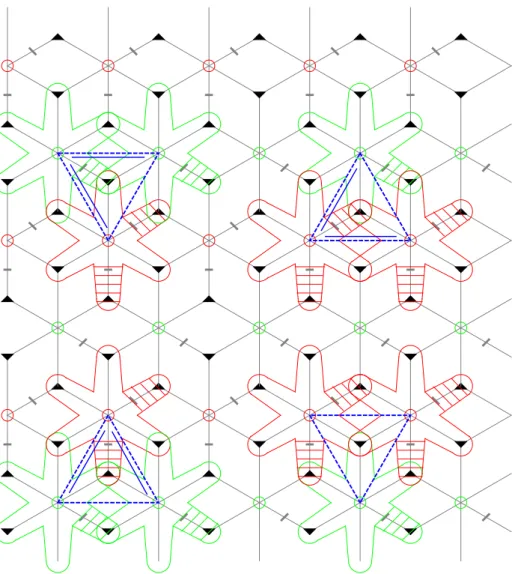
Figure 3.2: The four different configurations of three localized states in the lower band, where a (blue) triangle has been drawn between the centering sites of the states. The overlap between the states will depend on the weights of the rim sites in the triangle, and these are different for the two types of localized states (red and green). The sign of the total overlapσii_jk, resulting in the sign of the interaction, will then depend on which corner iof the triangle considred. Two operators will be centered on one of the overlapping states, the corner site i, while the other two states have one operator centered on them. These four different triangles are combined to form the effective lattice in figure 3.1.

3.3. Fermions 25

3.3

Fermions

In the Fermi-Hubbard model the on-site interaction takes the form: ˆ Hint=U X i ˆ ρi,↑ρˆi,↓=U X i ˆ c†_i,↑ˆci,↑cˆ†i,↓cˆi,↓, (3.11)

where an interaction of strength U arises as two particles with spins of opposite signs occupy the same site i. Due to the Pauli principle only one particle of a specific spin can occupy a site. The maximum energy per site is then U for the fermionic interaction. The projection onto the operators of the lowest band ¯ci, as

in the previous section, will result in an effective Hamiltonian given by: ¯

Hint=

X

i,j,k,l

Vijkl¯c†_i,↑¯cj,↑c¯†k,↓¯cl,↓. (3.12)

The projection of the operators for the fermionic case is the same as for the bosonic case since the real-valued gauge results in only real weights of the localized wave-functions. All the values of the pre-factorsVijklare then the same as for the bosons. However, due to the fermionic commutation relations and the spin label several of the combinations of operators that in the bosonic case lead to the same processes will here be split up into different terms. From here on the fermionic operators for the flat band are declared as ˆwi = ¯ci. A minus sign has now been added to the interaction, so that bothU∗andU∆are attractive interactions. If all contributions

(see Appendix B) are combined the effective Hamiltonian becomes: ¯ Hint = − U∗ 4 + U∆ 24 X i ¯ ρi,↑ρ¯i,↓ +U∆ 72 X hi,ji h ˆ w_i†_,↑wˆi,↓wˆj†,↓wˆj,↑+ ˆwj†,↑wˆj,↓wˆi†,↓wˆi,↑ i −U∆ 72 X hi,ji [ ¯ρi,↑ρ¯j,↓+ ¯ρi,↓ρ¯j,↑] −U∆ 72 X hi,ji h ˆ w_i†_,↑wˆ_i†_,↓wˆj,↓wˆj,↑+ h.c. i −U∆ 144 X ∆=i,j,k σiijk h ¯ ρi,↑wˆ†j,↓wˆk,↓+ ¯ρi,↑wˆ†k,↓wˆj,↓+ ˆw†k,↑wˆj,↑ρ¯i,↓+ ˆw†j,↑wˆk,↑ρ¯i,↓ i −U∆ 144 X ∆=i,j,k σii_jkhwˆ†_i,↑wˆ†_i,↓wˆk,↓wˆj,↑+ ˆw†i,↑wˆ † i,↓wˆj,↓wˆk,↑+ h.c. i +U∆ 144 X ∆=i,j,k σii_jkhwˆ†_i,↑wˆi,↓wˆ†k,↓wˆj,↑+ ˆw†i,↑wˆi,↓wˆ†j,↓wˆk,↑+ h.c. i , (3.13) whereσii

jk =±1 and are given by which triangle that the interaction acts on, see equation (3.10). A visual representation of the interactions can be found in figures

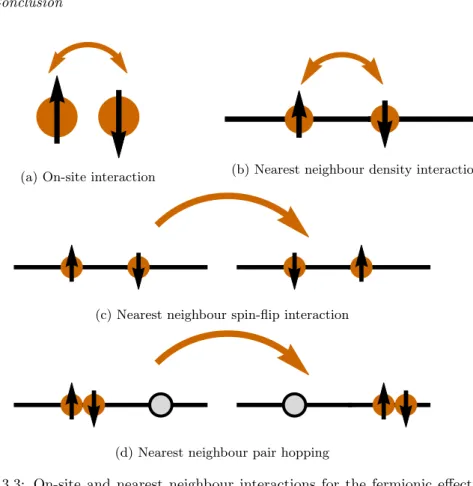
3.3 and 3.4. The first term in equation (3.13) is an on-site density term that results in a large negative contribution when two particles of opposite spins are located at the same site. The second, third and fourth terms act on nearest neighbour sites in the lattice. The second term is a spin-flip term that flips the spins of two neigh-bouring particles. Due to the Pauli exclusion principle this will only be possible for sites with single particles, so this terms does not act on pairs. The third term is a nearest neighbour density interaction. This term gives a contribution when particles of opposite spins are placed on neighbouring sites. The fourth term is a pair hopping term. If two particles of opposite spin are placed on the same site these can hop as a pair to a neighbouring empty site.

The fifth, sixth, and seventh terms act on two particles placed on the same tri-angle. The sign of the interaction depends on which triangle and on which sites that the interaction takes place. The fifth term is an assisted hopping term. If a particle with up-/down-spin is placed on siteiof a triangle another particle of spin down/up can hop between the two other sites of the triangle. The sixth term is a pair breaking/creation term. A pair on sitei of a triangle can break up into two single particles at the two other sites on the same triangle. The Hermitian conju-gate of this process represents two single particles, with opposite spins, forming a pair at the third site. Finally, the seventh term is a spin-rotation term. For two particles of opposite spins on different sites of the triangle can rotate one site, in the clock-wise or anti-clock-wise direction.

3.4

Conclusion

Effective Hamiltonians for both the bosonic and the fermionic case have been con-structed for the localized states in the lowest bands. The projection from the general on-site Hubbard interaction is given by the geometry of the lattice and the overlap of the chosen Wannier functions. The interactions in the effective Hamiltonians include an on-site interaction, nearest neighbour interactions, and interactions on a triangle. For the interactions on a triangle the sign of the interaction depends on over which bond on the triangle the interaction takes place. These signs are given in the effective lattice and are a consequence of the π-flux of the original lattice, see figure 3.1.

To now evaluate what the low-energy states are, the effective models should be studied for either repulsiveU > 0 or attractiveU <0 interactions. The resulting phases for each case will differ since the dominating terms that can lower the energy will not be the same. The fermionic model with attractive interaction will here be studied further. The Hamiltonian will then have several interaction terms that can lower the energy and the on-site term will dominate due to its size compared to the other smaller terms. Since the model is attractive the effects from forming pairs will first be studied by mapping the model containing only pairs onto a spin model.

3.4. Conclusion 27

(a) On-site interaction (b) Nearest neighbour density interaction

(c) Nearest neighbour spin-flip interaction

(d) Nearest neighbour pair hopping

Figure 3.3: On-site and nearest neighbour interactions for the fermionic effective Hamiltonian.

(a) Assisted hopping (b) Pair breaking/creation

(c) Spin rotation

Figure 3.4: Interactions on triangles for the fermionic effective Hamiltonian. For every process there exists a process for the opposite spins, as well as the Hermitian conjugate terms.

Chapter 4

Spin Mapping

From here on the fermionic effective model will be considered for attractive interac-tions. For the attractive case the term in the effective Hamiltonian that can lower the energy most is by far the on-site interaction. States that only contain pairs are then of interest as they are expected to dominate in the low energy states. Under the assumption that the states will have sites that are either empty or are occupied by a pair, the model can be mapped onto a spin-1/2 model. It has been shown that an attractive fermionic model on a flat band always can be mapped onto a ferro-magnetic spin-1/2 model as pair-breaking terms are truncated [3]. A pair of two fermions will have the properties of a hard-core boson, due to the Pauli principle, meaning that two pairs cannot occupy the same site. The mapping to a spin state can then be done by a spin-boson mapping [22]. Zero and pair occupation can be mapped onto spin down and spin up as follows:

|0ii → |+1₂ii

| ↑↓ii → | −1₂ii.

(4.1)

The mapping of the operators from fermion pairs to spin-1/2 operators becomes: ˆ S_i+↔wˆ†_i↑wˆ_i†_↓ Sˆ−_i ↔wiˆ↓wiˆ↑ Sˆiz↔ 1 2 ˆ w†_i↑wiˆ↑+ ˆwi†↓wiˆ↓−1 , (4.2) where the spin operators act on spin states as:

ˆ Sz

i|Sizii=Siz|Sizii ˆ S_i+|Sizii= p S(S+ 1)−Siz(Siz+ 1)|Siz+ 1ii ˆ S_i−|Sizii = p S(S+ 1)−Siz(Siz−1)|Siz−1ii. (4.3)

The ladder operators ˆS+_i and ˆS_i− will raise and lower the spins. For a spin-1/2 model the possible values areS= 1/2 andSiz=±1/2. The commutation relations

for spin operators are: h ˆ S_i+,Sˆ_j−i=δij2 ˆSzi h ˆ S_i±,Sˆjz i =∓δijSˆ_i±. (4.4) If only pairs of particles are considered the terms of the effective Hamiltonian (equation (3.13)) that will act on those states are:

¯ H_intpair= − _U ∗ 4 + U∆ 24 X i ¯ ρi,↑ρ¯i,↓ −U∆ 72 X hi,ji [ ¯ρi,↑ρ¯j,↓+ ¯ρi,↓ρ¯j,↑] −U∆ 72 X hi,ji h ˆ w†_i,↑wˆ†_i,↓wˆj,↓wˆj,↑+ ˆwj†,↑wˆ † j,↓wˆi,↓wˆi,↑ i . (4.5)

By inserting the mapping into spin operators (see Appendix C) the interacting Hamiltonian (equation (4.5)) for fermions becomes:

¯ H_intpair= −U∆ 36 X hi,ji ˆ Si·Sˆj − _U ∗ 4 + U∆ 24 + 3 U∆ 36 X i ˆ S_iz −1 2 _U ∗ 4 + U∆ 24 + 3 U∆ 72 , (4.6)

which can be written as: ¯ H_intpair= −J1 X hi,ji ˆ Si·Sˆj−h X i ˆ S_iz+C, _(4.7) withJ1= U₃₆∆,h= U₄∗+U₂₄∆ + 3U₃₆∆ , andC=−1 2 U∗ 4 + U∆ 24 + 3 U∆ 72 . The model is now a ferromagnetic Heisenberg model with a magnetic field in thez-direction. Energy will be gained in this model by aligning spins in the same direction from the spin exchange and the energy can be lowered further by setting the direction of spins to the up-direction, due to the magnetic fieldh. Generally a ferromagnetic model is to be expected from attractive fermions. However, that the resulting model becomes a Heisenberg model depends on the interaction strengths of each terms given from the projection.

4.1. Heisenberg model 31

4.1

Heisenberg model

If the more general case is considered, with an on-site interactionU, a pair-hopping t, and a nearest neighbour interactionV, the equation (4.5) after the spin mapping (see equation (C.5) in Appendix C) can be written as:

¯ H_intpair = −UX i ˆ Siz+ 1 2 −V X hi,ji ˆ SizSˆjz+ 1 2 ˆ Szi + ˆSjz +1 4 −2tX hi,ji 1 2 h ˆ S_i+Sˆ_j−+ ˆS_i−Sˆ_j+i= = −UX i ˆ S_iz−X hi,ji VSˆ_izSˆ_jz+ 2t1 2 ˆ S_i+Sˆ−_j + ˆS_i−Sˆ_j+ −V X hi,ji 1 2 ˆ Siz+ ˆSjz +1 4 −U 2 = = −X hi,ji VSˆ_izSˆ_jz+ 2t1 2 ˆ S+_i Sˆ−_j + ˆS_i−Sˆ_j+ −(U+ 3V)X i ˆ S_iz−1 2 U+ 3V 2 . (4.8)

It is only for the exact valueV = 2t, which is the value given from the effective model whereV = U∆

36 and t=

U∆

72, that the spin Hamiltonian can be rewritten as

a Heisenberg Hamiltonian with an applied magnetic field: ¯ H_intpair= −2tX hi,ji ˆ Si·Sˆj −(U+ 6t)X i ˆ S_iz−1 2(U+ 3t). (4.9)

The eigenstates to the part of the effective Hamiltonian that acts on the subspace with only pairs can be given as those of a ferromagnetic Heisenberg model. Since the hopping model is solved for a fixed number of particles the corresponding spin-eigenstates are those given by a fixed magnetization. Compared to the hopping model the spin model does not take the total number of particles, here total number of spin-ups, into account. To consider the effect of a specific filling of the lattice a chemical potential term should be added.

4.2

Chemical potential

To set the total number of particles in the hopping Hamiltonian a chemical potential term can be added:

ˆ Hchem=

X

i

[µ↑ρˆi,↑+µ↓ρˆi,↓]. (4.10)

For only pair occupation the density of spin up and spin down particles will be the same as the pair density and the spin mapping is written as ˆρi,↑= ˆρi,↓= ˆρi,↑ρˆi,↓=

ˆ S_iz+1₂, so that: ˆ Hchem= 1 2(µ↑+µ↓) + (µ↑+µ↓) X i ˆ S_iz. (4.11)

The chemical potential for spin up and spin down particles can be assumed to be equalµ↑=µ↓=1₂µ, resulting in:

ˆ Hchem= µ 2 +µ X i ˆ Siz. (4.12)

The spin Hamiltonian from equation (4.6) then becomes: ¯ H_intpair= −U∆ 36 X hi,ji ˆ Si·Sˆj − _U ∗ 4 + U∆ 24 + 3 U∆ 36 −µ X i ˆ S_iz −1 2 _U ∗ 4 + U∆ 24 + 3 U∆ 72 −µ . (4.13)

The effect of the chemical potential in the spin model is that the term can modify the magnetic field in thez-direction. The chemical potential then corresponds to setting a fixed magnetization of the model by fixing the number of spin-ups. Without setting a fixed magnetization the ground state of the ferromagnetic spin model will be a state where all spins are pointing in same direction. To correspond to the hopping model of a certain filling the magnetization should be set to correspond to the number of particles considered.

4.3

Conclusion

For states of the effective Hamiltonian that only contain pairs the model can be mapped onto a spin-1/2 Heisenberg model. For this case the entire effective model then simplifies to a ferromagnetic Heisenberg model. To consider the correct ground states all fillings of the lattice can be calculated by finding the ground state of the spin model at a fixed magnetization. The ground state of the ferromagnetic Heisenberg model will be a state where all spins are aligned. If a magnetic field is added the aligned spins will all point in that direction. For a model with a

4.3. Conclusion 33

fixed magnetization the number of up-spins is fixed. This corresponds to having a specific number of particles in the hopping model. Since no sites are more likely than others to have a spin in a specific direction the ground state for a specific number of up-spins will be degenerate, as these can be placed on any combination of sites. If the assumption that only pairs exist in the ground state is valid the state of the full model can easily be found at any filling. The entire Hamiltonian should now be considered to see to what extent this simplification is justified to use for the system. Since there are terms in the full effective Hamiltonian that split up pairs it is required that those effects are small. In the following chapter the full effective model will be considered at low filling. The pair-breaking terms are treated as a perturbation and their effect is approximated.

Chapter 5

Few-particle problem

In order to study the low-energy properties of the system the ground state is to be found. In the effective Hamiltonian for fermions, equation (3.13), there are several types of interaction from which energy can be gained. Due to the effective inter-actions being given by the projection of an attractive on-site interaction several of the interactions in the effective Hamiltonian can lower the energy of the system. To characterize the effects from the interactions, in this chapter the ground states at low filling are studied. The two-particle problem is first used to study the effects of creating pairs compared to instead gaining energy from the inter-site interactions between single particles. To characterize the states when several pairs can be in-volved, so that inter-site interactions between pairs occur, the four particle problem is then studied. As no interactions act on more than two filled sites at once these two cases can give some hint to the general characteristics of the many-body states at higher filling.

To study the full effective Hamiltonian it will be considered in two parts so that it can be treated with second order perturbation theory. Since the interaction con-stant for the on-site interaction U∗

4 +

U∆

24

and the nearest neighbour interaction U∆

72

are more than or twice as large as those for the triangular terms U∆

144

, the formation of pairs is expected to be dominant. However, the interaction constants for the terms on triangles are not small enough in comparison to be neglected. The triangular terms still include terms that can spilt up pairs. Treating these terms as a perturbation should give the order of corrections from single particle states to the ground state of only pairs. The effective fermionic Hamiltonian is divided into two parts as:

ˆ

H = ˆH0+ ˆH0, (5.1)

where ˆH0are the terms with the largest coefficients, the on-site and nearest neigh-bour interactions: ¯ H0= − _U ∗ 4 + U∆ 24 X i ¯ ρi,↑ρ¯i,↓ +U∆ 72 X hi,ji h ˆ w_i†_,↑wˆi,↓wˆj†,↓wˆj,↑+ ˆwj†,↑wˆj,↓wˆi†,↓wˆi,↑ i −U∆ 72 X hi,ji [ ¯ρi,↑ρ¯j,↓+ ¯ρi,↓ρ¯j,↑] −U∆ 72 X hi,ji h ˆ w_i†_,↑wˆ_i†_,↓wˆj,↓wˆj,↑+ ˆw†j,↑wˆ † j,↓wˆi,↓wˆi,↑ i (5.2)

and the perturbation is the interactions taking place on a triangle:

¯ H0= −U∆ 144 X ∆=i,j,k σ_jkii hρ¯i,↑wˆj†,↓wˆk,↓+ ¯ρi,↑wˆk†,↓wˆj,↓+ ˆw†k,↑wˆj,↑ρ¯i,↓+ ˆw†j,↑wˆk,↑ρ¯i,↓ i −U∆ 144 X ∆=i,j,k σ_jkii hwˆ_i†_,↑wˆ_i†_,↓wˆk,↓wˆj,↑+ ˆw†i,↑wˆ † i,↓wˆj,↓wˆk,↑+ h.c. i +U∆ 144 X ∆=i,j,k σ_jkii hwˆ_i†_,↑wˆi,↓wˆk†,↓wˆj,↑+ ˆw†i,↑wˆi,↓wˆj†,↓wˆk,↑+ h.c. i . (5.3) Here the unperturbed Hamiltonian ¯H0 is the same as for the spin mapping but

including a spin-flip term that only acts on single particles. The ground state for the unperturbed Hamiltonian is expected to consist of pairs of particles while the perturbation includes terms that break up pairs into single particles.

If the ground state is expected to lie in the subspace of only pairs then the effects of the perturbation creates states in the separate subspace of states containing single particles. Second order perturbation theory is a suitable approach since it eval-uates the off-diagonal elements between the eigenstates of ˆH0. The second order

correction to the ground state energy is given by:

E₀(2)= X m6=0 (H₀0_m)2 E0−Em = X m6=0 |h0|H¯0|mi|2 E0−Em , (5.4)

where all states |ni are eigenstates of ˆH0 with |0i being the ground state [23].

The ground state energy should be lowered by the perturbation. The amount it is lowered with, compared to the unperturbed ground state, will depend on the strength of the perturbation and which states|mithat results in non-zero elements H₀0_m.

5.1. Two-particle problem 37

5.1

Two-particle problem

The problem with two particles in the lattice, one spin up and one spin down, is first considered. These two particles can occupy the same site as a pair or sit as single particles at different sites. Since the on-site interaction term is much larger than the other it can be assumed that the ground state for ¯H0 will be found for

two particles forming a pair. The terms of ˆH0 when it acts upon a pair can be

expressed as: ˆ H₀pair=− _U ∗ 4 + U∆ 24 −µ −U∆ 72 X hi,ji h ˆ d†_idˆj+ ˆd†jdˆi i , (5.5)

where ˆd†_i = ˆw_i†_,↑wˆ_i†_,↓and ˆdi= ˆwi,↓wˆi,↑are pair creation and annihilation operators

that follow bosonic commutation relations. The unperturbed Hamiltonian can then be described as a simple hopping problem for the pair:

ˆ H₀pair=−tX hi,ji h ˆ d†_idˆj+ h.c i +C, (5.6) wheret= U∆ 72 andC=− U∗ 4 + U∆ 24 −µ

. The resulting dispersion relation for the triangular lattice will be:

(k) =−2t(cos (k1) + cos (k2) + cos (k3)) +C. (5.7)

The ground state will then have the energy: E₀(0) =−6t+C, given by thek = 0 case. The ground state is given by|0(0)_i

k= ˆd†k=0|vaciwhich with an inverse Fourier

transform becomes: |0(0)i=X i 1 √ Nsites ˆ w_i†_,↑wˆ_i†_,↓|vaci, (5.8)

which is a pair uniformly distributed over all sites in the lattice. If the perturbation ˆ

H0 now acts on this state we get: ˆ H0|0(0)_i= = √ 1 Nsites  − U∆ 144 X ∆=i,j,k σ_jkii hρ¯i,↑wˆj†,↓wˆk,↓+ ¯ρi,↑wˆk†,↓wˆj,↓+ + ˆw†_k,↑wˆj,↑ρ¯i,↓+ ˆw†j,↑wˆk,↑ρ¯i,↓ i −U∆ 144 X ∆=i,j,k σ_jkii hwˆ_i†_,↑wˆ_i†_,↓wˆk,↓wˆj,↑+ ˆwi†,↑wˆ † i,↓wˆj,↓wˆk,↑+ + ˆw†_j,↓wˆ†_k,↑wˆi,↑wˆi,↓+ ˆw†k,↓wˆ † j,↑wˆi,↑wˆi,↓ i X β ˆ w†_β,↑wˆ†_β,↓|vaci= = √ 1 Nsites  − U∆ 144 X ∆=i,j,k σ_jkii hδiβwˆk†,↑wˆj,↑wˆ†i,↑wˆ † i,↓+δiβwˆj†,↑wˆk,↑wˆ†i,↑wˆ † i,↓ i −U∆ 144 X ∆=i,j,k σ_jkii hδiβwˆ_k†_,↓wˆ_j†_,↑nˆi,↑nˆi,↓+δiβwˆj†,↓wˆ † k,↑nˆi,↑ˆni,↓ i  |vaci= = −√ 1 Nsites U∆ 144 X ∆=i,j,k σiijk h ˆ w†_k,↓wˆ_j†_,↑+ ˆw_j†_,↓wˆ_k†_,↑i|vaci= = −√ 1 Nsites U∆ 144 X ∆,∇=i,j,k,i0 σ_jkii +σ_jki0i0 hwˆ†_k,↓wˆ_j†_,↑+ ˆw†_j,↓wˆ†_k,↑i|vaci= 0. (5.9) This expression becomes zero sinceσ_jkii =−σ_jki0i0 for all opposite triangles ∆(i, j, k) and ∆(i0_{, j, k) due to the structure of the effective lattice (see figure 5.1). Notably,}

this state is then an eigenstate to ˆH0 as well as ˆH0. The state|0(0)iis the ground

state to the full Hamiltonian with the eigenvalueE₀(0)=− U∗

4 + U∆ 24 −6U∆ 72.

For states that only consist of single particles at different sites several eigenstates can be found. The two following states can be constructed for particles at neigh-bouring sites: |m(0)₊ i= √1 2 ˆ w†_a,↑wˆ_b†_,↓+ ˆw†_b,↑wˆ_a†_,↓|vaci |m(0)₋ i= √1 2 ˆ w†_a,↑wˆ_b†_,↓−wˆ†_b,↑wˆ_a†_,↓|vaci, (5.10)

which due to the nearest neighbour density interaction and spin-flip term are eigen-states to the Hamiltonian ˆH0:

ˆ H0|m(0)₊ i=−2U∆ 72|m (0) + i+µ|m (0) + i, Hˆ0|m (0) − i= 0|m (0) − i. (5.11)

These states are however not eigenstates to ˆH0 and therefore not either to the full Hamiltonian.

5.1. Two-particle problem 39

a

b

i

i'

Figure 5.1: Two single particles, with spins up and down, placed at a bonda, bare part of the triangles ∆(i, a, b) and ∆(i0, a, b). The effective lattice is structured so that for all bondsσii

ab=−σ i0i0 ab .

Single particles that are located further apart will not be affected by ˆH0 or ˆH0

and are therefore eigenstates with eigenvalue 0. It can from here be seen that no state has lower energy than the state|0(0)iand that it then is the ground state.

5.1.1

Corresponding spin state

The spin mapping results in the Hamiltonian in equation (4.6). If the single-pair ground state of the hopping Hamiltonian is given by (equation (5.8)):

|0(0)i=√ 1 Nsites X i ˆ w_i†_,↑wˆ_i†_,↓|vaci, (5.12) the corresponding spin state becomes:

|0(0)iS= √ 1 Nsites X i ˆ S+_i |vaci. (5.13)

The eigenvalues of these two states will be the same due to the relation:

X j ˆ S_jz|0(0)iS=X j ˆ S_jz√ 1 Nsites X i ˆ S_i+|vaci= = 1 2(N↑−N↓) 1 √ Nsites X i ˆ S_i+|vaci= 1 2(2−Nsites)|0 (0)_i S. (5.14)

As the magnetization of the spin system is set to 1₂N↑−N↓ Nsites = 1 2 1−(Nsites−1) Nsites = 1 2 2 Nsites−1