DEBT CONTRACTS AND LOSS GIVEN DEFAULT
Dan Amiram
A dissertation submitted to the faculty of the University of North Carolina at Chapel Hill in partial fulfillment of the requirements for the degree of Doctor of Philosophy in the Kenan-Flagler School of Business.
Chapel Hill 2011
Approved by: Robert M. Bushman Wayne R. Landsman Jeffery Abarbanell John R. Graham Mark H. Lang
ii ABSTRACT
DAN AMIRAM: Debt Contracts and Loss Given Default (Under the direction of Robert M. Bushman and Wayne R. Landsman)
This study explores how accounting information available to lenders at the contracting date shapes debt contracts by facilitating lenders’ assessment of loss given default (LGD). LGD, defined as the percentage loss experienced per $1 of debt if default occurs, is closely related to the notion of liquidation value which is central to debt
contracting theories. LGD, together with probability of default, determines expected credit loss and as such is a critical component of debt contract design. While a large literature examines probability of default, much less is known about the impact of expected LGD on contract design and the information set relevant to lenders in assessing LGD at debt
iii
iv
ACKNOWLEDGEMENTS
v
TABLE OF CONTENTS
LIST OF TABLES ... vi
DEBT CONTRACTS AND LOSS GIVEN DEFAULT ... 1
Introduction ... 1
Motivation, background and predictions ... 7
Data and sample ... 16
Empirical design and results ... 19
Sensitivity tests ... 35
Conclusion ... 37
Appendix A – Definitions ... 39
Appendix B – Simple model of LGD and credit spreads ... 42
vi
LIST OF TABLES Table
1. Descriptive statistics ... 44
2. The relation between accounting measures at the debt issuance date and future LGD ... 46
3. The relation between PREDICT_LGD and SPREAD ... 47
4. The relation between PREDICT_LGD and SPREAD over and above default likelihood ... 48
5. The effects of default likelihood on the relation between PREDICT_LGD and SPREAD ... 49
6. The effects of managerial entrenchment on the relation between PREDICT_LGD and SPREAD ... 50
7. The relation between PREDICT_LGD and SECURED ... 51
8. The relation between PREDICT_LGD and time to Maturity ... 52
9. The relation between PREDICT_LGD and debt size ... 53
10.The effect of the precision of the accounting signal on the relation between PREDICT_LGD and SPREAD ... 54
1. Introduction
This study explores how accounting information that is available to lenders at the contracting date shapes the design of debt contracts. I posit that an important channel through which accounting information affects contracts is by facilitating lenders’ assessment of loss given default (LGD). LGD, defined as the percentage loss lenders experience from $1 of outstanding principal in a case of default, is closely related to the notion of liquidation value and is a critical component of credit risk and debt contracting theories.1 Despite the theoretical importance of LGD, there is little empirical evidence on its effects on debt contracts. Even rarer is evidence regarding how information available to lenders at the contracting date shapes their expectations about LGD and, in turn, affects debt contract terms.
In this study I exploit a dataset of loss given default realizations to estimate a prediction model based on financial accounting information available to lenders at the loan contracting date. I then use this model to study the impact of accounting-based LGD expectations on the design of debt contracts. Specifically, for a sample of defaulted debt instruments, I first examine the extent to which financial accounting information available prior to the contracting date predicts lenders’ losses in cases where default occurs. Using the LGD prediction model developed in the first step, I generate an accounting-based measure of expected LGD at loan initiation dates for a large sample of non-defaulted borrowing firms. I then examine whether expected loss given default affects key terms of the debt contract such as interest rate spread, maturity, security and debt size, and also when expected loss given default has stronger effects on lenders. I further examine how
1
2
sectional differences in characteristics of firms’ accounting information affect the extent to which lenders use the information about loss given default when they initiate the debt contract.
According to credit risk theory, the price and terms of risky debt depends directly on lenders’ assessments of expected losses from the instrument. Expected credit loss is generally conceptualized as the product of the probability of default and expected loss given default.
Although a substantial body of research focuses on predicting and evaluating the effects of default probabilities, only recently, as necessary data have became available, has research started to investigate determinates and consequences of LGD. In addition, LGD is intimately related to a firm’s liquidation value, where higher liquidation value implies lower LGD. Liquidation value is central to many debt contracting theories, since the optimal debt contract depends on how costly it is for lenders to liquidate the borrower’s assets. Higher liquidation values alleviate some of the lenders’ concerns about incentive conflicts they have with borrowers (Aghion and Bolton, 1992; Hart and Moore, 1994).
Although these arguments suggest that LGD is important to lenders, there are reasons why firm-specific information about LGD may not be useful for debt contracting. For example, some
studies suggest that firm-specific LGD is diversifiable (Altman, 2009). In addition, anecdotal evidence suggests that lenders do not use firm-specific information to estimate LGD (Gupton and Stein, 2005). Moreover, accounting information available to lenders at the date of the contract (47 months on average before the default date in my sample) may not have power for predicting LGD. Despite its theoretical importance, there is lack of empirical evidence on the relation between LGD and debt contract terms.2 Of particular interest to this study is the fact that little documented
evidence exists regarding how lenders collect, assess and use information on LGD and liquidation value at the contract date.
2
3
This study seeks to provide direct evidence on the link between firm-specific information, LGD and debt contract characteristics such as credit spread, maturity, size and security. A key source of firm-specific information available to lenders at the contract decision date is accounting information from the borrower’s financial statements (Tirole, 2007; Standard and Poor’s, 2009). I conjecture that publicly available financial statement information available to lenders at the contracting date is useful to predict loss given default. I focus on available contracting date
accounting information to provide insights into how accounting-based estimates of LGD explain the revealed structure of contracts. Although accounting information at the default date can be used to estimate loss given default, such estimates are ex post in nature and cannot be used to infer how lenders make their lending decision.
I utilize a sample of senior unsecured defaulted bonds for which data on LGD realizations and accounting information in the year before the issuance of the bond exist to construct a
prediction model for LGD. The analysis finds that five accounting measures explain a high proportion of the variation in LGD.3 Cross-validation test results show that the model has significant predictive power for realized LGD out-of-sample. I use the coefficients from the
prediction model to construct an expected LGD estimate for all non-defaulted, nonconvertible bond issuances in the Securities Data Company (SDC) database with available accounting information at the date of the issuance.
Using these estimates of expected LGD, I next investigate the extent to which LGD affects debt contract design. I expect that interest spreads will be higher for borrowers with higher
predicted LGD as lenders will demand compensation for the increased expected losses. Using a
3
4
model that includes extensive control variables such as contract terms and industry and year fixed effects, I find that expected LGD is associated with higher credit spreads at the bond issuance date. Expected LGD continues to be a statistically and economically significant determinant of spread after including controls for the probability of default such as the Vassalou and Xing (2004) DLI measure, Altman’s Z score and S&P credit rating. The results suggest that a one standard deviation increase in LGD expectation adds 58 basis points to the interest rate spread of the debt.
Because LGD manifests only when the borrower defaults, I expect its effect on credit spreads to be stronger when the probability of default is higher. If the probability of default is zero LGD does not matter. However, if the probability of default is close to one, LGD should matter a lot. I also predict that the effect of LGD on debt contracts will be stronger when borrowers have the ability to extract private benefits (Aghion and Bolton, 1992). Consistent with these predictions, I find that the effect of the predicted LGD on spread is stronger when the probability of default is higher and when the entrenchment index of the issuer from Bebchuk, Cohen and Ferrell (2008) is higher.
Spread is not the only contract term likely to be affected by LGD expectations. Lenders may require collateral when they expect LGD to be higher. In addition, lenders may shorten the maturity of loans with higher expected LGD as the higher frequency of re-contracting will allow creditors to refuse contract renewal, ask for a better security or require an increase in interest rate when expected credit losses have increased. Lenders may also place limits on loan amounts for firms with higher expected LGD to limit their exposure to LGD.4 I find evidence consistent with these predictions.
4
5
I next examine how the precision of accounting information impacts the sensitivity of credit spreads to accounting-based LGD estimates. It is plausible that lenders place more reliance on accounting information in predicting LGD as the precision of the information increases. Appendix B presents a simple analytical model that shows how LGD and information about LGD affects the credit spread. I find that lenders are more sensitive to predicted LGD when contracting with firms characterized as having high value-relevance and timelier accounting. In contrast to arguments in the literature, lenders are more sensitive to the predicted LGD in firms with less conservative accounting.5,6
Although private loans differ in many respects from public bonds, I use a sample of private loan issuances to provide evidence that analogous relations between expected LGD and debt contracts also hold in this setting after controlling for financial covenant strictness. In addition, I provide evidence that lenders use stricter covenants when LGD is expected to be higher.
The inferences above are robust to a variety of sensitivity tests, such as inclusion of credit rating fixed effects and different subsets of control variables. Using Monte-Carlo simulations, I also show that an LGD measure constructed using random coefficients with the same sign and magnitude as the coefficients from the prediction model performs poorly relative to the prediction model in explaining spreads. This suggests that the expected LGD measure constructed with the coefficients from the prediction model captures a latent structural variable that is distinct from the individual accounting measures used to estimate it. In addition, I include each of the accounting measures as a control variable and show that none of them affects the inferences described above.
5
This argument does not speak to the overall efficiency of a specific accounting system to debt contracting. Rather it speaks to the usefulness of an accounting system in the estimation of LGD, which is an important channel in debt contracting. However, as discussed in more detail below, other channels exist, for example lenders’ ability to estimate default likelihood.
6
6
This study contributes to the literature along several dimensions. First, I show that
accounting information available to lenders at the contracting date is significantly associated with future loss given default. To the best of my knowledge, this paper is the first to do so. Second, I construct an intuitive measure of LGD expectations at the time of debt initiation which could be of use in future research. Third, I show that accounting-based expectations about LGD significantly affect price and non-price terms of the debt contract. This finding contributes to the LGD and liquidation value literature by showing that LGD has significant non-diversifiable effects on debt contracts and to the accounting literature by showing a specific channel through which accounting information is useful in lending decisions. Fourth, this study contributes to the accounting debt contracting literature by providing evidence that lenders put more weight on LGD expectations from accounting systems that are more value-relevant, timely and less conservative. Lastly, the results of this study highlight the valuation role of accounting in debt contracting, by showing that accounting facilitates the estimation of LGD and by implication, liquidation values. This
7 2. Motivation background and predictions
A substantial body of research in accounting and finance focuses on modeling the likelihood of default. This literature uses accounting ratios (e.g., Beaver 1966; Altman, 1968; Ohlson, 1980) and variations of the Merton (1974) model (e.g., Vassalou and Xing, 2004; Bharath and Shumway, 2008), among other methods, to assess the probability of default. This literature also examines the implications of increased probability of default on debt pricing, equity pricing
(Vassalou and Xing, 2004) and debt policy. It is only recently that research about the second major component of credit risk, loss given default, has emerged.7
LGD, which is defined as the percentage loss lenders experience from $1 of outstanding principal in a case of default (or 1 minus the recovery rate), interacts directly with the probability of default in determining credit risk (Gupton and Stein, 2005). The credit risk modeling literature discusses how credit spreads or the prices of risky bonds and loans are determined as a function of probability of default and loss given default. Although credit risk models may differ significantly in their assumptions about LGD and its determinants, in all models LGD plays an important role in pricing credit risk.8
Fundamentally, a firm’s net assets and future cash flows provide implicit collateral to lenders. The liquidation value of the implicit collateral is a main determinant of LGD as liquidation value is inversely related to LGD. Since a borrower cannot commit not to withdraw his human
7
See Altman (2009) for a survey of this emerging literature. 8
8
capital (as in Hart and Moore, 1994) or not to divert cash flows (as in Aghion and Bolton, 1992), there is an incentive conflict between lenders and borrowers. Because of the incentive conflict, lenders will agree to provide funds to borrowers only if the default triggers liquidation. According to these models, the yield decreases in the assets’ liquidation value. This occurs because increased liquidation value reduces the cost of liquidation which, in equilibrium, reduces the spread charged by lenders. In addition, debt maturity increases with liquidation values since higher liquidation values increase the assets’ durability and make longer maturity feasible (Hart and Moore, 1994). Moreover, these models posit that the funds lenders are willing to provide is directly tied to assets’ liquidation values. Despite the importance of LGD in these models, as Benmelech et al. (2005) suggest, empirical evidence on this issue is scarce. In particular, there is very little evidence on how lenders obtain and use information about liquidation values and LGD.
The interest in this issue is exemplified by an important emerging literature. This literature utilizes unique settings to examine the link between liquidation value, collateral and debt
characteristics. Benmelech et al. (2005) focus on the redeployability of property assets as determined by commercial zoning regulation and find that more deployable properties receive larger loans, longer maturities and lower interest rates. Benmelech (2009) finds that assets’ salability in the 19th century railroad industry leads to longer maturities of debt. Benmelech and Bergman (2009) study a sample of loans in the airline industry and show that collateral and redeployability are negatively correlated with yield spread. I build on this literature by examining the link between information available to lenders at the date of the contract about LGD and debt contract characteristics in a more general setting.
9
accounting’s ability to capture credit deterioration affects the structure of syndicated loans. Graham et al. (2008) show that corporate misreporting leads to a sharp deterioration in debt contract terms for the misreporting firms. Several studies build on Watts (2003) and find evidence that
conservative accounting is generally beneficial to debt contracting by limiting the agency problem between lenders and borrowers (Zhang, 2008; Nikolaev, 2010). Sunder et al. (2009) provide evidence that spread is negatively associated with adjusted market to book ratio, suggesting that realized conservatism reduces risk by promoting lenders’ confidence in the collateral value of the firm’s assets. Recent theoretical studies take differing positions regarding whether conservative accounting increases debt contracting efficiency. Whereas Gox and Wagenhofer (2009) claim that the optimal accounting system for debt contracting is conservative, Gigler et al. (2009) and Li (2008) suggest that since conservative accounting also creates a loss of informativeness, it can reduce the efficiency of debt contracts.
Two recent survey studies call for additional research on these issues. Roberts and Sufi (2009) call for future research that links liquidation values or LGD and the structure of debt contracts. Armstrong, Guay and Webber (2010) review the accounting literature and suggest that lenders are likely to prefer more reliable accounting information to evaluate the firm’s collateral. Notably, none of the reviewed papers provide direct evidence to support this hypothesis.
Armstrong et al. (2010) also suggest that further research is needed to find the channels through which the quality of financial reporting affects debt contracts. One of the objectives of my paper is to explore such a channel.
10
(Gupton and Stein, 2005; Altman, 2009). This line of reasoning suggests that lenders that hold diversified debt portfolios may care only about LGD means across the economy or industry and not firm-specific LGD. A related point is that anecdotal evidence from practitioners suggests that lenders use “lookup tables” of historical LGDs based on industry and seniority type, as inputs for their lending decisions (Gupton and Stein, 2005). These lookup tables, based primarily on lenders’ experience, provide lenders with the historical LGD rate for a debt instrument for a given industry and seniority. Although Gupton and Stein (2005) note that lenders augment these historical tables with subjective judgment, the nature and the basis of these judgments is unclear. It is also unclear how representative this evidence is and how available information about firm-specific LGD is used in the lending process.
Third, since defaults occur several years after the contracting date, 47 months on average in my sample, accounting information at the contracting date may have no power for predicting future LGD. Fourth, because accounting information is not designed for the purpose of estimation of liquidation value that affects LGD, it therefore might be useless for this purpose. Fifth, lenders may use private information to estimate LGD and put less weight on publicly available financial
information. Lastly, LGD is inherently difficult to estimate as evidenced by the fact that lack of consistent empirical evidence on its distribution and importance have led analytical and empirical researchers to often assume LGD is constant across countries or industries, or ignore its role completely (see Acharya et al. 2004 for examples). This inherent difficulty in estimating LGD may cause lenders to use alternative measures to protect themselves against LGD loss. Therefore it remains an open empirical question whether firm-specific information is useful for lenders to assess LGD and whether it affects debt contracts.
11
financial ratios about the probability of default is the core of the seminal work of Beaver (1966), Altman (1968) and many subsequent studies (e.g., Ohlson, 1980 and Zmijewski, 1984). This work shows that information in financial statements can predict defaults. In addition, the LGD literature has suggested that certain accounting measures, when observed at the date of default, can predict LGD.9 I extend the insights from both literatures and conjecture that certain accounting measures available to lenders at the contracting date can also predict LGD. To the best of my knowledge, this study is the first to examine the relation between measurs based on accounting information that is available to lenders at the debt issuance date and LGD.10
I use five accounting measures to predict LGD on a sample of 308 defaulted senior unsecured bonds.11 I use a homogenous set of senior unsecured debt instruments to make sure the accounting measures I use do not capture differences in the seniority and security of debt. Using secured instruments as the benchmark for the prediction model may create measurement problems with assessing the value and nature of the pledged security. In addition, senior unsecured debt is the most common form of debt in the default and LGD dataset (Moody’s Default Risk Services,
9
Varma and Cantor (2005) and Acharya et al. (2007) find some relation between accounting measures and LGD around the default event. Jacobs and Karagozoglu (2007) use a larger sample and different accounting measures and find stronger evidence for this relation.
10
The largest rating agencies have only recently started issuing independent LGD (recovery rate) ratings for debt instruments. These ratings are not available for many firms and were not available to lenders for most of the years in the sample. In addition, some of these ratings are available only after the contract was designed. As Gupton (2005) discusses, a primary goal of Moody’s LGD “LossCalc 2” model is to help lenders to assess LGD for bank regulatory provisioning purposes required by the Basel accord.
11
12
DRS database) and the bond issuance data (SDC) that I use in this paper.12 The five accounting measures I use are extracted from financial reports published in the year before debt issuance to ensure the information was available to lenders. The measures and their predicted associations with LGD are based on the intuition suggested in papers that predict LGD with data contemporaneous to the default event (Acharya et al. 2005; Varma and Cantor, 2005).
The first measure is earnings before interest and tax (EBIT) scaled by total assets (ROA). ROA is predicted to be negatively associated with LGD. All else equal, the more profitable the
firm, the greater the chance of lenders getting a higher price for selling the firm as a going concern or liquidating the assets. The second ratio is net book assets of the firm scaled by the number of shares outstanding (NET_WORTH). I predict a negative association between NET_WORTH and LGD. The greater the net assets of the firm, the more unencumbered assets lenders have available to sell and recover their investments. The third ratio is intangible to tangible assets
(INTANGIBLE_RATIO). Many intangible assets are difficult to transfer and thus may yield low value in liquidation, creating a positive association between INTANGIBLE_RATIO and LGD. The fourth ratio is short term debt to long term debt (STTOLTDEBT). This ratio should be positively related to LGD because short term lenders have the ability either to withdraw their funds from the firm in the near term or refuse to renew them and thus leave lower net assets for long term debt holders in case of default. The final measure is the log of total assets (LTA), which is a proxy for the level of complexity in the sale of a firm’s assets and thus the liquidity of those assets. In addition, this measure is associated with the complexity of the firm’s bankruptcy procedures in case of a default, which yields lower recovery rates and thus higher predicted LGD. In addition, I use Fama and French 17 industries classification indicators to capture industry effects on LGD.
12
13
After evaluating the association between the accounting measures and LGD, I next investigate how this information affects debt contract design. Holding probability of default constant, I expect that higher LGD will spur lenders to require higher interest rates to compensate for higher risk. Moreover, lenders should be more sensitive to LGD in firms that have a higher probability of default since LGD by definition occurs only if default occurs. Lenders will use all relevant information to assess expected LGD, including accounting information, and will be more sensitive to signals that provide more precise information about LGD. Appendix B presents a simple analytical model that shows how LGD and information about LGD affects the credit spread.
To examine these predictions, I use the estimated coefficients on the five accounting
measures and industry indicators in the prediction model to construct an LGD expectation measure. The measure, PREDICT_LGD, is constructed for a sample of all non-defaulted, non-convertible bond issues in the U.S, available on the SDC new issuances database. The measure is effectively the predicted value of LGD using the accounting information available to lenders before the contract is designed. I expect PREDICT_LGD to be positively associated with interest rate spread over the treasury benchmark (SPREAD). Further, PREDICT_LGD should have a distinguishable effect from measures of probability of default, and it should have a stronger effect on firms that have a higher probability of default.
Theory also predicts that the effect of liquidation value and LGD on debt contracts will be larger when borrowers have the ability to extract private benefits (Aghion and Bolton, 1992). Thus I expect that the positive association between PREDICT_LGD and spread will be stronger when managerial entrenchment is expected to be higher. The reason for that is that managerial
14
I also examine the effect of PREDICT_LGD on whether security is required in the debt contract. If expected LGD is high, lenders will require borrowers to pledge specific assets against the loan to protect against loss in case of default. Thus, I expect the probability of secured
borrowing to increase with PREDICT_LGD. In addition, LGD risk may cause lenders to shorten the maturity of the debt in order to better monitor the situation of the firm and facilitate withdrawal of the funds in cases where the probability of default is increasing. This creates a negative expected association between PREDICT_LGD and the maturity of debt. Because lenders may limit their exposure to firms with high LGD risk, I expect a negative association between PREDICT_LGD and the size of the debt relative to the firm’s assets. These additional tests help mitigate concerns that lenders have multiple contracting options to protect themselves against future losses.13
Consistent evidence on the directional effect of expected LGD across these different debt contract characteristics helps to draw stronger conclusions on the observable effects.
Finally, I predict that PREDICT_LGD will have a stronger effect on SPREAD in firms whose accounting information provides a more precise signal on LGD. However, it is not obvious which properties of accounting information reflect more precision with respect to predicting LGD. One possibility is that accounting systems that recognize economic losses in a more timely manner (more conservative) also provide more precise information to lenders about LGD, since this conservative system is designed to provide information about the lower bound of liquidation value (Watts, 2003; Sunder et al. 2009). On the other hand, accounting information that more strongly predicts changes in equity value may also reflect more precise information to lenders about the value of the net assets available to them in case of default and thus more precise information on LGD. I examine both possibilities.
13
15
Although the prediction model for LGD uses a sample of defaulted bonds, I also assess the effects of PREDICT_LGD on a sample of bank loan issuances. Bank loans are different in many aspects from corporate bonds but the line of reasoning regarding the relations between LGD and debt contract features applies to bank loans as well. Most importantly, banks have the ability to ask for information over and above what is provided in financial statements, in addition to the fact that the cost of renegotiation is lower relative to public bonds. Using LGD expectation based on
defaulted bonds makes PREDICT_LGD a noisy proxy for LGD expectations for bank loans. These additional analyses help to increase the external validity of the PREDICT_LGD measure and to improve understanding about whether the mechanism of adjusting debt contracts to expected losses based on accounting information works similarly in private and public debt issuances. In addition, using this sample allows me to control for financial covenant strictness and to examine the
16 3. Data and sample
I use information about actual LGD’s contained in Moody’s DRS database. The data contain information on over 1,000 defaults as well as information on 30-day recovery pricing, which is the price of the bond 30 days after the default event. These data allows me to calculate LGD for defaulted bonds. All data are derived from Moody’s own proprietary database of issuer and default information. Moody’s analysts use these data to perform their own analysis and determine ratings and outlooks for all credits. The database provides the backbone for the Annual Default Study, read by more than 40,000 investors globally. According to Moody’s, the data are refreshed monthly to provide the most accurate, detailed portrait of default activity available in the market. A more thorough description of the data is provided in Varma and Cantor (2005).
I merge accounting information for the year before the bond was issued from
COMPUSTAT with the DRS dataset based on CUSIP. For reasons that are discussed above I keep only observations of defaulted senior unsecured bonds of non-bank corporations. This sample, which I refer to as the DRS sample, contains information on 308 defaulted bonds that have LGD and industry data as well as the data needed to calculate the five accounting measures used in the prediction model.14
Table 1 Panel A provides descriptive statistics for the DRS sample. On average, bonds lose 67 percent of their face value, an amount which is consistent with prior literature (Varma and Cantor, 2005). At the date of issuance, firms are on average profitable (mean ROA of 0.05) and have high NET_WORTH (Mean of 10.84). On average, firms in the DRS sample have more intangible than tangible assets (mean INTANGIBLE_RATIO of 2.57); however, the median of INTANGIBLE_RATIO is 0.25, which suggests that most of the firms in the DRS sample have more
tangible than intangible assets. 14
17
The second step of the analysis requires data on bond issuances that never defaulted.
Following Bharath et al. (2008), I obtain data on public bonds from the Securities Data Corporation (SDC) new issuances database. I use data for bond issuances for the period 1988-2008 and exclude convertible bonds. Consistent with prior literature, I also exclude bonds with maturities that are shorter than one year as well as those issued by banks. I merge the data from SDC with accounting data for the year before the issuance from COMPUSTAT based on CUSIP. I require an observation to have all data required for the bond characteristics, PREDICT_LGD, and control variables in order to be included in the data. I also eliminate approximately 100 observations that have
PREDICT_LGD that is larger than one or smaller than zero.15 The final sample, which I refer to as the “Bond sample”, contains 3,599 bond issuances.
Table 1 Panel B provides descriptive statistics for the bond sample. On average the bonds in this sample have a 200 basis point spread over the treasury benchmark. The calculated expected LGD for this sample has a mean of 0.69. The firms in the bond sample are profitable (mean ROA of 0.1) and 62 percent of them are above investment grade.
I also utilize a sample of private debt issuances to test the effects of LGD expectations on debt contracts. The sample of private debt issuances is obtained in a similar manner to Bharath et al. (2008) and to the bond sample above. I obtain data for this sample from the Dealscan database provided by Loan Prices Corporation. I use all available loans (facilities) in Dealscan with maturity longer than 12 months for the period 1988-2006.16 I merge the data from Dealscan to accounting data for the year before issuance from COMPUSTAT based on the link table described in Chava and Roberts (2008).17 I require an observation to have all data required for the loan characteristics, PREDICT_LGD, and control variables in order to be included in the sample. I also eliminate
15
Including these observations does not change any of the inferences described below. 16
I stop the sample at 2006 because this is the last Dealscan dataset that is available to me. 17
18
approximately 300 observations that have PREDICT_LGD that is larger than one or smaller than zero.18 This sample, which I refer to as the “Loan sample”, contains 13,325 loan facilities.
Table 1 Panel C provides descriptive statistics for the loan sample. On average the loans in this sample have a 183 basis point spread over the Libor benchmark. The calculated expected LGD for this sample has a mean of 0.63. The firms in the loan sample are profitable (mean ROA of 0.08). Only 49 percent of the loans have a long term debt rating available in COMPUSTAT, while only 20 percent of the sample have higher than investment grade rating.
18
19 4. Empirical design and results
The empirical design is comprised of several stages. First I examine the association
between accounting measures at the debt issuance date and LGD. The second stage uses the results from the first stage to estimate PREDICT_LGD. The third stage examines the association between PREDICT_LGD and debt contract characteristics as well as how different accounting systems
affect this relation.
4.1 The predictive ability of accounting measures at the contract date about future LGD
To empirically assess whether there is an association between accounting ratios and future losses, I estimate the following equation using OLS.19
LGDid, is loss given default at the default date, and is calculated using data from Moody’s DRS
dataset as one minus the recovery rate. Where the recovery rate is the price of the instrument one month after the default occurred divided by the face value of the instrument. This method is consistent with practitioner and academic research (Acharya et al. 2004; Varma and Cantor, 2005; Gupton and Stein, 2005), and yields unbiased measure for LGD since there is an active market for defaulted debt for a few months after the default which allows traders to buy and sell the defaulted instrument (Gupton and Stein, 2005).
The five accounting measures I use are ROA, NET_WORTH, INTANGIBLE_RATIO, STTOLTDEBT and LTA. These measures and their expected associations with LGD are described
19
Since the dependent variable, LGD, is between zero and one, OLS estimated coefficients may be biased. Logit transformation and Pepke and Wooldridge (1996) estimation methods were also used. These methods yield similar results to the ones using OLS, thus for simplicity of the calculations and interpretation I use OLS. In addition, if the coefficients that I based my expected LGD on are biased it would be harder for me to obtain results in the following tests.
(1)
LGDid = 0 + 1* ROAi,t-1 + 2* NET_WORTHi,t-1 +
20
more thoroughly in section 2 above.20ind are industry indicator variables for each of the
Fama-French 17 industries classification.21 The industry indicators capture mean differences in LGD between different industries and allow the accounting measures to capture differences between firms that are not related to industries. Appendix A discusses the sources of data for the variables.22
I estimate equation (1) on the DRS sample described in section 3. Table 2 presents the results from this estimation. Model 1 presents the estimation of equation (1) without industry fixed effects, Model 2 presents the estimation of the regression with just the fixed effects and none of the accounting measures, while Model 3 provides results for the estimation using accounting measures and fixed effects.
The results from the estimation of Model 1 show that the five accounting measures provide information to lenders about LGD. Model 3 suggests that the accounting measures are significant determinants of LGD over and above the industry means that many lenders use as predictors (Gupton and Stein, 2005). As expected ROA is negatively associated with LGD (coefficient of -0.907 with a t-statistic of -4.88 in model 1, and coefficient of -0.781 with a t-statistic of -4.11 in model 3), which suggests that firms that were more profitable at the issuance date have higher recovery rates. NET_WORTH is also negatively associated with LGD (coefficient of -0.005 with a t-statistic of -3.94 in model 1, and coefficient of -0.004 with a t-statistic of -2.79 in model 3), which as predicted suggests that the greater the net assets of the firm, the lower the losses debt holders incur in case of default. INTANGIBLE_RATIO, STTOLTDEBT and LTA are all positively and
20
The only purpose of this prediction model is to construct an accounting based measure of LGD expectation at the contracting date. Thus I do not claim these measures are the only ones or the best ones to explain LGD and I acknowledge that the prediction model may be improved in future research. I found these measures to be intuitive, available for most firms on COMPUSTAT and statistically sufficient for the analysis presented in this paper. 21
The industry classification is available on Ken French’s website. 22
21
significantly associated with future LGD. INTANGIBLE_RATIO has a coefficient of 0.003 with a t-statistic of 5.04 in model 1 and a coefficient of 0.003 with a t-t-statistic of 4.17 in model 3, which suggests that firms with higher intangible assets relative to their tangible assets are valued less in case of default. STTOLTDEBT has a coefficient of 0.018 with a t-statistic of 2.79 in model 1 and a coefficient of 0.025 with a t-statistic of 2.71 in model 3. This result is consistent with the ability of short-term lenders to pull out their funds in a more timely manner relative to long-term lenders and thus leave the firm with lower net assets in case of default. LTA has a coefficient of 0.063 with a t-statistic of 5.83 in model 1 and a coefficient of 0.062 with a t-t-statistic of 5.07 in model 3. This result is consistent with the fact that the bankruptcy proceedings are more complicated when firms have more assets and that selling more assets in case of default requires larger liquidity discounts.
Model 2 is presented to show that the adjusted R-squared of the estimation of only fixed effects (industry means) is slightly smaller than the adjusted R-squared of using only the
accounting measures (R-squared of 0.17 compared to 0.18). More generally, the accounting measures have significant predictive power regarding LGD by themselves (R-squared of 0.18) but more so when industry fixed effects are used (R-squared of 0.28). Taken together the results in table 2 suggest that information in the financial statements, available to debt investors at the issuance date, has significant predictive ability about future LGD.23
4.2 Constructing LGD expectation measure-PREDICT_LGD
I use the coefficients from the estimation of equation (1) to construct PREDICT_LGD. Using the bond sample described in section 3 above, I multiply each estimated coefficient from equation (1) by the relevant accounting measure in the year before the bond issuance and add them
23
22
together with the relevant industry intercept to obtain PREDICT_LGD for every bond in the sample. For example PREDICT_LGD for a firm j from industry z that issued a bond in a year t is given by equation (2).
where i are the estimated coefficients from equation (1). 0 is the intercept obtained from equation (1) and z is the incremental industry intercept. I use the same method to construct PREDICT_LGD separately in the loan sample.
4.3 The relation between PREDICT_LGD and debt contract terms
To assess the relation between lenders’ expectation of LGD and debt contract characteristics, I follow a research design used extensively in the debt contracting literature (Bharath et al. 2008, Ivashina, 2008). Specifically, I estimate the association between PREDICT_LGD and the price and non-price characteristics of the debt contract.
4.3.1 The relation between PREDICT_LGD and SPREAD
To examine the relation between PREDICT_LGD and the price of debt, I start by estimating the following OLS regression.
where SPREAD is the interest rate spread over a treasury benchmark at the date of the bond issuance. PREDICT_LGD is the estimated predicted LGD for the bond that is obtained from equation (2). X is a vector of variables used frequently in the literature to control for other determinants of the credit spread. X includes the size of the issuer (LSIZE), the leverage of the issuer (LEV), the issuer’s growth opportunities (Q), the size of the debt issuance
PREDICT_LGDjt= 0+z+1* ROAj,t-1+ 2* NET_WORTHj,t-1
+ 3* INTANGIBLE_RATIOj,t-1 + 4* STTOLTDEBTj,t-1 + 5* LTAj,t-1,
(2)
23
(LFACEAMOUNT), the maturity of the debt (LMATURITY), an indicator variable for secured debt (SECURED), an indicator variable for above investment grade debt (INV_GRADE), and an
indicator variable for rated debt (SPRATED). and are industry and year fixed effects, respectively. The presence of industry fixed effects in equation (3) isolates the firm-specific expected LGD from the industry level to identify a unique firm-specific information effect. Appendix A provides further description on the source and construction of the variables.24
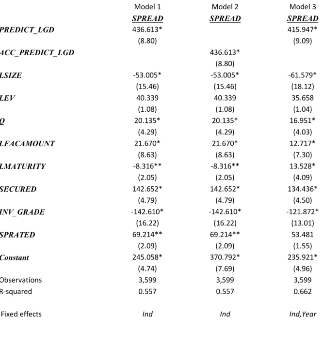
Results from estimating equation (3) on the bond sample are presented in table 3. Model 1 presents the estimation of equation (3) with industry fixed effects and excludes year fixed effects. Model 2 constrains the industry estimators in the construction of PREDICT_LGD to be zero, which effectively uses only the accounting measures to create the ACC_PREDICT_LGD measure. By construction, all the coefficients in Model 2, except for the intercept, should be identical to the coefficients in Model 1. Model 2 is included to show that constraining the industry coefficients to be zero is identical to using industry fixed effects. Model 3 presents the estimation of equation (3) with industry and year fixed effects. For the sake of brevity, I discuss only the implication of the results of model 3 and highlight the differences from other models.
The estimation results in model 3 show that PREDICT_LGD is positively and significantly associated with SPREAD (coefficient of 415.9 with a t-statistic of 9.09). This result is consistent with the explanation that lenders use information about LGD available to them in the financial statements to price debt. The accounting information as reflected in PREDICT_LGD explains the cross-sectional variation in SPREAD incremental to any industry effect, as is clear from the industry fixed effects estimation and from model 2.25 The effect is economically significant where
24
Although they are generally not included in debt contracting research design, in untabulated results, I add to all estimated models described in this paper the equity characteristics annual returns and standard deviation of monthly returns. The addition of these variables does not change any of the inferences described in this paper.
25
24
a one standard deviation change (14%) in PREDICT_LGD translates to a 58 basis point change in SPREAD which is 29.1% of the SPREAD mean. This result suggests that LGD expectations have a
significant economic effect on the pricing of debt contracts.26,27
4.3.2 The effect of PREDICT_LGD and SPREAD over and above default likelihood
A concern is that PREDICT_LGD, or more generally loss given default, is correlated with default likelihood. A positive correlation between PREDICT_LGD and default likelihood is likely since in distressed periods, firms may be forced into fire sales of their assets and liquidation values at these unfavorable times (Shleifer and Vishny, 1992; Acharya et al. 2008).28 Thus, an important feature of the research design is to distinguish between PREDICT_LGD and default likelihood. I use three different measures of default likelihood to isolate the effect of PREDICT_LGD. I use the Vassalou and Xing (2004) default likelihood indicator (DLI), Altman’s (1968) Z score multiplied by negative one (Z), and a numeric conversion of S&P long term rating (SPRATING). All measures are constructed in a way that their respective higher values are proxies for higher likelihood of default. Although all three measures are proxies for likelihood of default, they are all constructed very differently, which allows me to better identify the unique effect of expected LGD on the contract. DLI is based on the Merton (1974) model and is constructed using information in stock prices, debt and assets. Z score is constructed using accounting ratios that were shown to have predictive ability about future defaults. SPRATING is based on debt analysts’ forecasts about the quality of the firm’s long term debt.
26
For the sake of brevity, I do not discuss the results of the control variables estimates for any of the estimations in this study except in cases where these results are important to the purposes of this paper. However, I note that these estimates are generally consistent with prior literature.
27
When I include the five accounting measures in these tests instead of the constructed measure of predicted LGD, I find that some the accounting measures are insignificant in explaining spread. In addition, the five accounting measures do not add to the explanatory power of the model compared to models that include the predicted LGD measure. 28
25
To assess whether the effect of PREDICT_LGD is over and above the default likelihood, I estimate a variation of equation (3) by adding each of the default likelihood controls one by one and then adding all of the three measures to the regression at the same time.29 If PREDICT_LGD indeed captures the construct of expected loss given default it should have a distinct effect on SPREAD that is over and above the probability of default. This feature of LGD is also a clear
prediction from the model described in Appendix B.
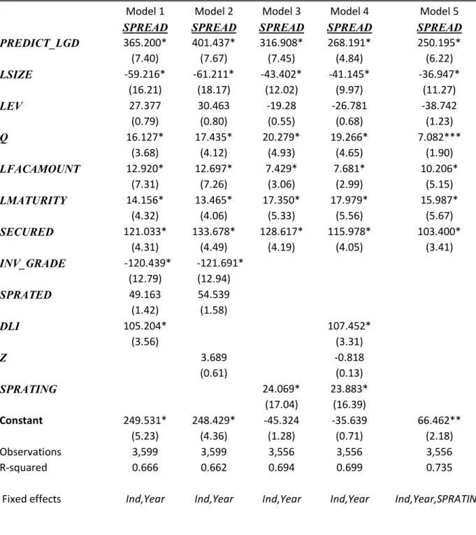
Table 4 presents results from these tests. Model 1 includes DLI as a control variable, Model 2 includes Z, and Model 3 includes the S&P credit rating. Model 4 includes all three additional control variables in the regression. Model 5 uses the S&P ratings as fixed effects to estimate the effects of LGD on SPREAD within a rating group, i.e., the coefficient on PREDICT_LGD in this estimation comes from the variation that is not related to credit risk as represented by S&P credit ratings. In all models, the coefficient on PREDICT_LGD is still statistically and economically significant. Model 5 is where the coefficient on PREDICT_LGD is the lowest (250.1) and has with a t-statistic of 6.22.30 Model 4 is where the t-statistic of the PREDICT_LGD coefficient is the lowest (4.84) with a coefficient value of 268.19. Taken together the results in table 4 suggest that PREDICT_LGD has an incremental, significant effect on debt pricing over and above the
probability of default.
4.3.3 The effect of default likelihood on the relation between PREDICT_LGD and SPREAD
Since losses to debt holders occur only when a default event occurs, I expect SPREAD to be more sensitive to PREDICT_LGD when the likelihood of default is higher. In the extreme case when the probability of default is zero, loss given default means very little to debt investors. However, when the probability of default is close to one, debt investors should put higher weights
29
This assumes the relation between probability of default and LGD is linear. In the next section I relax this assumption.
30
26
on how much they would be able to recover. To examine this effect I partition my sample into two groups of high and low default likelihood. I partition the sample based on each of the default likelihood proxies, i.e., one partition that is based on below and above the median of DLI, a second partition that is based on below and above the median of Z, and a third partition that is based on below and above INV_GRADE. I then estimate equation (3) for each of the groups for every partition variable. For the reasons suggested above, I expect the coefficient on PREDICT_LGD, 1, to be greater in the high likelihood of default group than it is in the group where the likelihood of default is lower.31 The comparison of the coefficients across partitions is done using a Monte-Carlo non-parametric simulation technique where I randomly assign observations into the partitions and take the difference between the coefficients 1,000 times.32
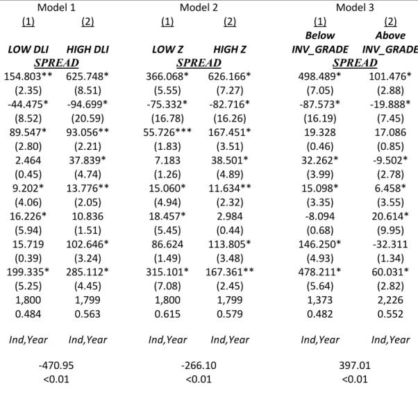
The results of this analysis are presented in table 5. Model 1 presents estimations based on the partition of over and above the median DLI. Model 2 presents estimations based on the
partition of over and above the median Z. Model 3 presents estimations based on the partition of below and above investment grade. As predicted, in Model 1, the coefficient on PREDICT_LGD in the high DLI bonds (625.7) is larger than the coefficient on PREDICT_LGD in the low DLI bonds (154.8) where the difference (470.95) is significant at the 1% level. In Model 2, the coefficient on PREDICT_LGD in the high Z bonds (626.2) is larger than the coefficient on PREDICT_LGD in the
low Z bonds (366.1) where the difference (260.1) is significant at the 1% level. In Model 3, the coefficient on PREDICT_LGD in the below investment grade bonds (498.5) is larger than the coefficient on PREDICT_LGD in the above investment grade bonds (101.5) where the difference
31
This design is conceptually similar to the use of a design that includes in the regression an indicator variable for high probability of default, PREDICT_LGD and their interaction, including the interaction of all control variables with the indicator variable.
32
27
(397.0) is significant at the 1% level. All three models are consistent with the prediction that when the probability of default is higher, lenders are more sensitive to expected LGD.
4.3.4 The effect of managerial entrenchment on the relation between PREDICT_LGD and
SPREAD
Theory predicts that lenders will rely more on liquidation values and LGD when agency conflicts between lenders and borrowers are greater. To assess whether lenders require higher interest rate compensation for LGD risk when agency conflicts are greater, I merge my sample with the entrenchment index (EINDEX) from Bebchuk et al. (2008) at the year of the bond issuance. This index captures insiders’ ability to extract private benefits from the corporation. I partition my sample into high entrenchment and low entrenchment issuers based on the sample median of EINDEX, reestimate a variation of equation (3) for each partition, and test for the difference in the
coefficients between groups. As above, the test of the difference between the coefficients across partitions is based on Monte-Carlo simulation.
The results of this analysis are presented in table 6. As predicted, the coefficient on PREDICT_LGD in the high EINDEX corporations (378.5) is larger than the coefficient on
PREDICT_LGD in the low EINDEX (178.6) where the difference (199.9) is significant at the 5%
level. This result is consistent with lenders putting more emphasis on liquidation values when the potential for private benefits extraction is greater.
4.3.5 The relation between PREDICT_LGD and the probability of secured debt borrowing
28
where SECURED and PREDICT_LGD are as defined above. As discussed earlier, the coefficient on PREDICT_LGD, 1, is expected to be positive. C is a vector of the control variables. and are industry and year fixed effects, respectively.
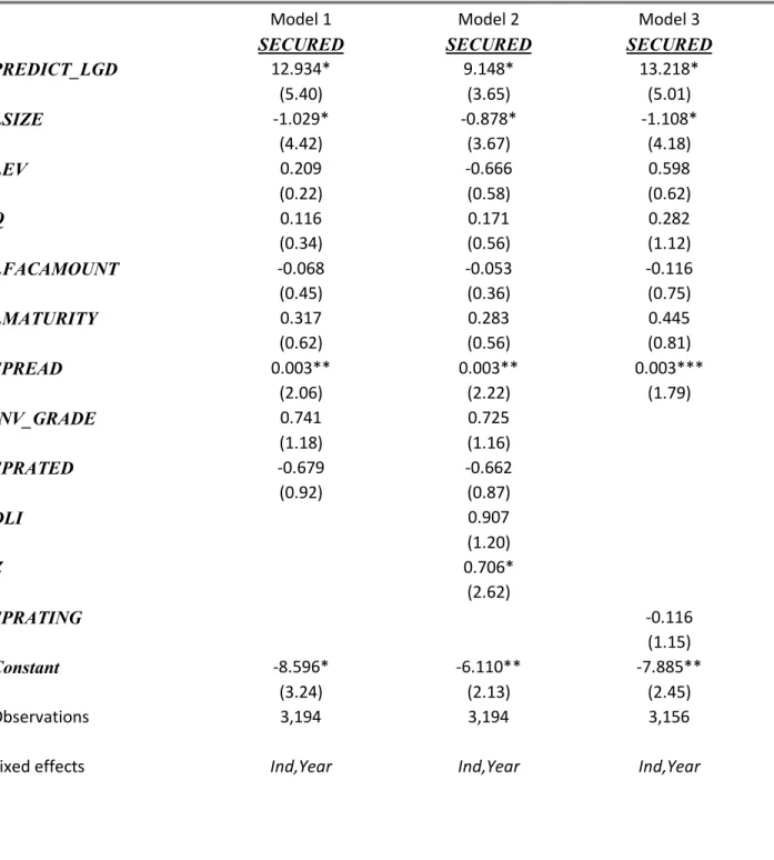
Table 7 presents results from estimating equation (4). Model 1 includes only a binary variable for above investment grade firms as a control variable for probability of default. Model 2 includes two additional variables, DLI and Z, as controls for probability of default and model 3 includes SPRATING as a control. In all three models PREDICT_LGD is positively and
significantly associated with the probability a bond will be secured (coefficients of 12.9, 9.1, and 13.2 with z-statistics of 5.4, 3.6 and 5.0 in Models 1, 2 and 3 respectively). This finding is consistent with lenders demanding a specific security against their investments when expected losses are larger. Such security may reduce lenders’ exposure to LGD.
4.3.6 The relation between PREDICT_LGD and debt maturity
Another measure that lenders can take to reduce their exposure to LGD is to provide funds with shorter maturity. The reason shorter maturity reduces lenders’ exposure to LGD is that it enables them to assess the likelihood of default with greater frequency. If the borrower has high expected LGD, the lender will want to monitor the borrower’s probability of default more often so if an increase in default likelihood occurs, the lender is able to refuse renewal of the contract. To assess this possibility, I estimate the following OLS regression.
where LMATURITY and PREDICT_LGD are as defined above. As discussed earlier, the coefficient on PREDICT_LGD, 1, is expected to be negative. P is a vector of control variables and and are industry and year fixed effects, respectively.
(4)
LMATURITYit = 0 + 1* PREDICT_LGDi,t-1+ 2* Pi,t-1+++, (5)
29
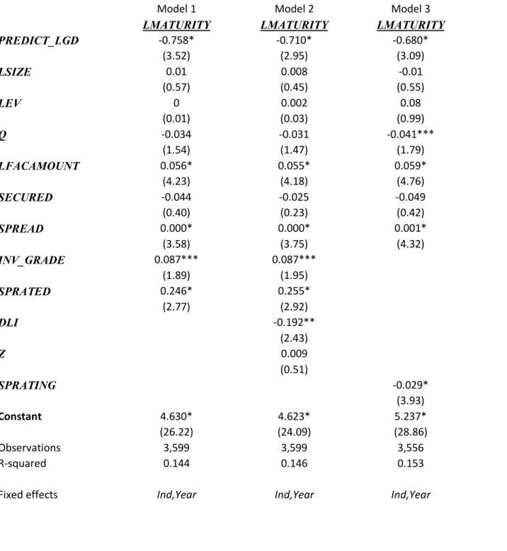
I present the results from these tests in table 8. Model 1 includes only a binary variable for above investment grade firms as a control variable for probability of default. Model 2 includes two additional variables, DLI and Z, as controls for probability of default and model 3 includes
SPRATING as a control. In all three models PREDICT_LGD is negatively and significantly
associated with the length of the debt contract (coefficients of -0.758, -0.710, -0.680 with t-statistics of -3.5, -2.9 and -3.1 in Models 1, 2 and 3 respectively). This finding is consistent with lenders being willing to lend funds for shorter time periods when the expected losses in case of default are higher. This may occur because lenders want to monitor the debt for higher
PREDICT_LGD firms more closely and frequently.
4.3.7 The relation between PREDICT_LGD and debt size
The liquidation value literature has suggested that lenders may place limits on loan amounts for firms with low liquidation value. Lenders may want to limit their exposure to LGD risk and thus provide fewer funds to high LGD firms. To examine this possibility I estimate the following OLS regression.
where SDEBTSIZE is the face value of the debt divided by the borrower’s total assets. PREDICT_LGD is as defined above. For the reason discussed above, the coefficient on
PREDICT_LGD, 1, is expected to be negative. E is a vector of the various variables used in the literature to control for other determinants of debt size. and are industry and year fixed effects, respectively.
I present the results from these estimations in table 9. Model 1 includes only a binary variable for above investment grade firms as a control variable for probability of default. Model 2 includes two additional variables, DLI and Z, as controls for probability of default and model 3 includes SPRATING as a control. PREDICT_LGD is negatively and significantly associated with
30
the size of the debt in all models (coefficients of 0.202, 0.246 and 0.214 with tstatistics of 2.5, -2.8 and -2.5 in Models 1, 2 and 3 respectively). This finding is consistent with lenders supplying fewer funds to lenders with high expected LGD in order to limit their exposure.
4.3.8 The effect of the precision of the accounting signal on the relation between PREDICT_LGD and SPREAD
If accounting provides an informative signal about LGD to debt investors, then, investors should put more weight on accounting predictors of LGD from accounting systems that provide more precise information about it.33 The qualities of an accounting system that generates more precise signals on LGD is an empirical question. I use measures for three accounting system qualities, RELEVANCE, TIMELINESS and CONSERVATISM, to address this question.34 These qualities are commonly used in the accounting literature with some variation in the way the measures are constructed. I follow Francis et al. (2004) in the construction of the measures. Although all three measures have compelling justification for why they should provide more precise information on LGD, they capture inherently different characteristics. RELEVANCE is the explanatory power from a regression of concurrent stock returns on earnings and changes in earnings. More formally, RELEVANCE is the R-squared from the following regression, estimated for a firm-specific time series for firms with a maximum of 10 years and a minimum of 4 years of available data before the debt issuance.
where RET is the cumulative return for the 15 months ended 3 months after the fiscal year end. NIBEX is net income before extraordinary items and ΔNIBEX is the change in net income before
extraordinary items. The construct RELEVANCE attempts to capture how well an accounting system captures changes in the value of the firm.
33
In this paper I use the terms signal precision and signal quality interchangeably.
34
See a discussion on the construction of these measures below.
31
TIMELINESS is the explanatory power from a regression of earnings on concurrent returns,
an indicator variable for negative returns and the interaction between the two. More formally, TIMELINESS is the R-squared from the following regression, estimated for a firm-specific time
series for firms with a maximum of 10 years and a minimum of 5 years of available data before the debt issuance.
where RET and NIBEX are defined above and D is an indicator variable that takes the value of 1 when RET is negative. This measure is aimed to capture how timely earnings are, or how earnings capture the information in concurrent news.
CONSERVATISM is the coefficient on bad news from equation (5) relative to the
coefficient on good news from equation (5). More formally CONSERVATISM is defined as (λ 3 + λ
2)/λ 2. CONSERVATISM attempts to capture how timely a firm recognizes bad news.
I partition my sample based on high and low values, based on the median, of each of the three accounting system characteristics, RELEVANCE, TIMELINESS and CONSERVATISM. I then estimate equation (3) separately for each of the high and low groups. If an accounting system characteristic provides more precise information on LGD then the coefficient on PREDICT_LGD, 1, should be greater in the high group than in the low group and vice versa.35 As in section 4.3.3, the comparison of the coefficients across partitions is preformed using a Monte-Carlo
non-parametric simulation technique.
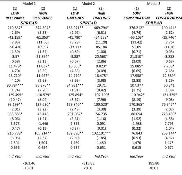
Table 10 provides results from the estimation of equation (3) based on partitions on the three proxies for information precision. Model 1 partitions the sample for high and low
RELEVANCE firms. The results of the estimation of Model 1 suggest that the coefficient on
35
A better strategy empirically to assess this question is to examine first the predictive ability of the LGD prediction model under each partition and then to test whether models with better predictive ability are weighted more heavily by investors. However, sample size limitations at the prediction model stage preclude using this strategy.
32
PREDICT_LGD in the high RELEVANCE firms (374.3) is larger than the coefficient on
PREDICT_LGD in the low RELEVANCE firms (210.8) where the difference (163.5) is significant
at the 1% level. This result is consistent with firms that have accounting systems that provide more relevant information about changes in firms’ market values, also provide more precise information to lenders about LGD.
Model 2 partitions the sample for high and low TIMELINESS firms. The results of the estimation of Model 2 suggest that the coefficient on PREDICT_LGD in the high TIMELINESS firms (469.8) is larger than the coefficient on PREDICT_LGD in the low TIMELINESS firms (154.0) where the difference (315.8) is significant at the 1% level. This result is consistent with the claim that firms that have accounting systems that provide information that better maps news (as represented by returns) into earnings, also provide more precise information to lenders about LGD.
On the contrary, Model 3 partitions the sample for high and low CONSERVATISM firms. The results of the estimation of Model 3 suggest that the coefficient on PREDICT_LGD in the high CONSERVATISM firms (190.4) is lower than the coefficient on PREDICT_LGD in the low
CONSERVATISM firms (376.2) where the difference (185.8) is significant at the 1% level.36 This result suggests that relevant, not conservative, accounting provides valuable information to lenders about liquidation values at the contracting date.
An interesting finding from table 10 is that firms with more conservative accounting systems provide more precise information to lenders about the probability of default. This can be seen from comparing the coefficients on DLI in model 3 between the high (coefficient of 222.5 with t-statistics of 4.58) and low conservatism (coefficient of 86.1 with t-statistics of 1.52) groups. However I leave the exploration of this channel to future research.
36
33 4.3.9 Bank Loans and PREDICT_LGD
Thus far, I have used a sample of bond issuances to assess the relation between LGD and debt contract characteristics. I next apply equation (2) to construct PREDICT_LGD for the bank loan sample described in section 3 above. Since the coefficients that comprise PREDICT_LGD are based on defaulted bonds, the measurement error of PREDICT_LGD in the bank loan sample is greater. However, this fact will tend to bias against finding results in this sample. I repeat the analysis on the relation between PREDICT_LGD and debt contract characteristics in the bank loan sample in an attempt to extend the external validity of my findings and to test whether the contract adjustment mechanisms for LGD work in loans and bonds similarly.
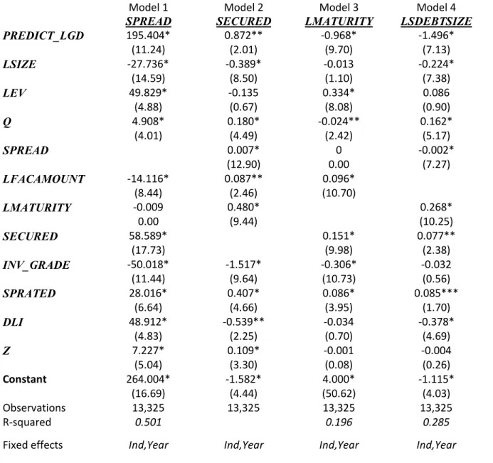
I present the results of these tests in table 11-Panel A. The results show that the main findings in the bond sample can be extended to the bank loan sample. Model 1 shows that PREDICT_LGD is positively associated with the spread over the Libor benchmark with a
coefficient of 195.4 and t-statistic of 11.24. Model 2 shows that PREDICT_LGD is positively associated with the probability a loan will be secured (a coefficient of 0.87 and t-statistic of 2.0). I also show, in Model 3, that the maturity of bank loans is negatively associated with
PREDICT_LGD (a coefficient of -0.97 and t-statistic of -9.70). Lastly, I show, in Model 4, that the
size of bank loans is negatively associated with PREDICT_LGD (a coefficient of -1.496 and t-statistic of -7.13).37 These results suggest that the mechanism through which LGD affects bond terms is similar to the mechanism through which it affects loan contracts.
Using to the bank loan sample also allows me to examine how financial covenants affect the results presented in this paper and to evaluate the relation between the strictness of the financial covenants and PREDICT_LGD. To do this, I use a measure of covenant strictness
(COV_STRICTNESS) which is based on Murfin (2010). This measure captures the ex-ante
37
34
probability of covenants violation based on how far the financial ratios are from the covenants and the standard deviation of the ratios. Table 11-Panel B presents the results of this exercise. Model 1 to Model 4 show that all the results that were documented in Table 11-Panel A hold after
35 5. Sensitivity tests
5.1 Does PREDICT_LGD capture the direct effect of the underlying accounting measures that comprise it on contracts, and how unique is the linear combination that comprises it?
One concern about the findings above is that any linear combination of the elements that comprise PREDICT_LGD will yield similar results. In other words, the question arises as to how unique is the linear combination the estimation of equation (1) provides. It may be that
PREDICT_LGD captures the direct effect of the accounting measures it is comprised of on the debt
contract (e.g., the direct relation between ROA and SPREAD or the direct relation between NETWORTH and SPREAD that is not operating through LGD). Since there are potentially an
infinite number of linear combinations for the coefficients, in an attempt to address these questions, I use a simulation technique.
The simulation proceeds as follows. I randomly choose a number from a uniform
distribution between zero and one for each of the five coefficients of the accounting measures that make PREDICT_LGD. To each random coefficient I attach the sign I obtained from equation (1). For example, the new random coefficient on ROA will be a number between negative one and zero and the new random coefficient on LTA will be a number between zero and one. I restrict the coefficients to be between zero and one because this is the range of the “true” coefficients obtained originally from equation (1). After obtaining the new five random coefficients, I recalculate
PREDICT_LGD for the bond sample using the new random coefficients. I estimate equation (3)
using the new PREDICT_LGD and check the significance level on its coefficient. I repeat this procedure 1,000 times.
Untabulated findings indicate that out of the 1,000 estimations, the coefficient on the new PREDICT_LGD is only significant 66 times at the 5 percent level and 0 times at the 1 percent
36
information about their range and sign. Out of 1,000 guesses, in only 66 attempts do I obtain a linear combination that significantly explains SPREAD.38
This finding is consistent with the claim that the information about the linear combination obtained from equation (1) is important and not just any linear combination of the coefficients will work. This also means that PREDICT_LGD does not capture by construction the effects of the underlying accounting measures on SPREAD.
5.2 Additional robustness and sensitivity tests.
I conduct numerous sensitivity tests. Among them are: adding each of the variables that comprise LGD to the regression as a control variable to test that none of them by itself significantly affects the inferences described above;39 adding the industry LGD means and the accounting
predicted LGD separately to the regressions; removing different subsets of control variables, including observations with PREDICT_LGD that are below zero and above one; adding DLI, yearly returns and standard deviation of monthly returns to the prediction model; and including yearly returns and the standard deviation of monthly returns as control variables to all tests. None of these additional tests change the inferences from the results presented above.
38
In an additional test I use a similar technique and choose four coefficients randomly and let the fifth coefficient, (ROA), be the one that allows PREDICT_LGD of the median firm in the sample and PREDICT_LGD of the median firm using the original “true” coefficients to be identical. I find that only in 16 cases the coefficient on PREDICT_LGD is statistically significant in explaining SPREAD.
39
37 6. Conclusions
This study addresses the effects of information available to lenders in the financial reports about loss given default at the contracting date on price and non-price terms of debt contracts. First, using a sample of defaulted senior unsecured bonds, I show that the information contained in five accounting measures that are available to lenders in the financial statements at the contracting date, is significantly associated with future LGD in a predictable manner. I use the estimation of the relation between these accounting measures and LGD to construct a measure of expected loss given default at the contracting date for non-defaulted debt instruments which I name
PREDICT_LGD. I predict, using a simple analytical model, and find that PREDICT_LGD is
positively associated with bond credit spread over the treasury benchmark. This relation is incremental to the effect of the probability of default on spreads. Moreover, as expected, the relation between PREDICT_LGD and credit spread is stronger when the probability of default and managerial entrenchment are greater. PREDICT_LGD is also strongly associated with non-price contract terms. Bonds of firms with higher expected LGD have a greater probability of being secured and having shorter maturity. In addition, bonds of firms with higher PREDICT_LGD are smaller relative to the borrower’s assets. I also use a sample of bank loan issuances to show that these findings hold after controlling for covenant strictness and that covenants strictness is higher when expected LGD is higher.