EFFECTS OF SPATIOTEMPORAL TEMPERATURE VARIATION ON BENTHIC COMMUNITY DYNAMICS IN THE GALAPAGOS ISLANDS
Lindsey Anne Carr
A dissertation submitted to the faculty at the University of North Carolina at Chapel Hill in partial fulfillment of the requirements for the degree of Doctor of Philosophy in the Department
of Biology.
Chapel Hill 2016
Approved by: John F Bruno
James Umbanhowar Robert Peet
ABSTRACT
Lindsey Anne Carr: Effects of spatiotemporal variation on benthic community dynamics in the Galapagos Islands
(Under the direction of John F Bruno)
Temperature can affect population and community level processes, via strong and predictable effects on individual metabolism. Metabolic Scaling Theory (MST) 1) describes how individual metabolic rates scale with temperature, and 2) generates mechanistic predictions based on how this response to temperature variation will drive ecological pattern and process. For example, temperature can influence trophic interactions via differential metabolic scaling of predator and prey metabolic rates. More specifically, metabolic theory and experiments indicate warmer temperatures can increase the top-down effects of herbivores on plant biomass, resulting in depleted standing plant biomass. Yet there are few studies that have tested metabolic scaling theory in the ocean across natural, in situ, environmental gradients.
For my doctoral dissertation research, I quantified benthic community patterns across the Islands and related community composition and biomass to temperature. I also tested metabolic scaling theory in the Galapagos Islands via lab experiments, in situ grazing assays, and a long-term exclusion experiment. Further, to examine the generality of temperature variation in
ACKNOWLEDGEMENTS
This work would not have been possible without the support and mentorship of John Bruno. He has inspired me and pushed me to be a better scientist. I would also like to thank my doctoral committee members, F Joel Fodrie, Jon Witman, Robert Peet and James Umbanhowar for their guidance. I am especially grateful for F Joel Fodrie and Jon Witman for their support in the field.
I am incredibly thankful for the many people at the Galapagos Science Center,
Universidad de San Francisco de Quito and the Galapagos National Park. In particular (and in no particular order) Steve Walsh, Courtney Butnor, Carlos Mena, Phil Page, Leandro Vaca, Diana Amoguimba, Luis Vinueza, Maryuri Yepez, Galo Quezada and Carlos Valle. The crews of the Pirata and the Oberlus II provided reliable access to my study sites; and I especially thank Captain Lenin Cruz Bedon and the Escarabay brothers. I am grateful for the field support from Pablo Mejia and Simon Villamar.
This dissertation would not have been finished without the support of my labmates, Courtney Cox, Abel Validivia and Rachel Gittman. You all have been a constant source of support, love and entertainment. A very special thanks to Rachel Gittman for traveling with me to the Galapagos multiple times for weeks on end, and putting out one fire after another. I also thank Emily Darling for reading drafts and discussing ideas with me. And I am very grateful to Ivana Vu, Pamela Reynolds and Courtney Cox for their tremendous support during my first few summers in the Galapagos.
Fund, UNC the Department of Biology and the Graduate School at UNC, the Phycological Society of America and the Center for Galapagos Studies.
TABLE OF CONTENTS
LIST OF TABLES...ix
LIST OF FIGURES...x
CHAPTER 1: Warming increases the top-down effects and metabolism of a subtidal herbivore...12
Introduction...12
Methods...14
Results...19
Discussion...20
Tables...24
Figures...25
CHAPTER 2: Temperature influences herbivory across a regional-scale temperature gradient in the Galapagos Islands, Ecuador...29
Introduction...29
Methods...31
Results...36
Discussion...37
Tables...45
CHAPTER 3: Spatiotemporal variation in thermal regimes and consumer assemblages infuences subtidal benthic communities across the Galapagos
Islands...51
Introduction...51
Methods...54
Results...58
Discussion...60
Tables...65
Figures...68
CHAPTER 4: Variation in thermal regimes and herbivore-algal interactions across upwelling systems...74
Introduction...74
Methods...77
Results...82
Discussion...87
Figures...92
LIST OF TABLES
Table 1.1 Natural variation in algal cover, temperature and urchin
density in shallow subtial habitats in the Galapagos Islands…...24
Table 2.1. Natural variation in site attributes. ...45
Table 2.2 Two-factor ANOVA and ANCOVA on control-corrected grazing rates...46
Table 2.3. One-factor ANOVA on final algal biomass...47
Table 3.1 Ranking of the 10 best generalized linear mixed models (GLMM) plus the null model for each response variable...65
Table 3.2 Model results for best-fit GLMM model based on AICc rankings...66
LIST OF FIGURES
Figure 1.1 Map of Galapagos Archipelago and the surrounding currents...25
Figure 1.2 Daily water temperature (mean) measured in the shallow subtidal (< 5m) at Santiago, Isabela and San Cristobal...26
Figure 1.3 Mesocosm temperature values during both experiments...27
Figure 1.4 Temperature effects on urchin grazing rates, metabolism and algal photosynthesis…...28
Figure 2.1. Map of the Galápagos Islands and the surrounding currents...48
Figure 2.2. Temperature effects on A) urchin and B) mobile and benthic herbivore consumption of Ulva...49
Figure 2.3. Herbivore effects on algal biomass...50
Figure 3.1 Map of the Galápagos Islands and the surrounding currents...68
Figure 3.2 Benthic community composition at cold and warm sampling periods...69
Figure 3.3 Relationship between temperature (°C) and macroalgal percent cover...70
Figure 3.4 Relationship between green urchin density and macroalgal percent cover...71
Figure 3.5 Results of nonmetric multidimensional scaling (NMS) ordination...72
Figure 3.6 Relationship between temperature (°C) and environmental parameters...73
Figure 4.1 Map of study regions and sites...92
Figure 4.2 Variation in ocean temperature across the regions ...93
Figure 4.3 Boxplot of weekly averaged mean temperature for 1999 – 2010...94
Figure 4.4Boxplot of weekly averaged mean temperature between years between 1999-2010...95
Figure 4.5Variation in spatial mean ocean temperature across the regions...96
CHAPTER 1: WARMING INCREASES THE TOP-DOWN EFECTS AND METABOLISM OF A SUBTIDAL HERBIVORE
Introduction
The strength of herbivore-plant interactions determines the composition and distribution of primary producers in many marine communities (Lubchenco & Gaines 1981, Hawkins & Hartnoll 1983, Paine 1992, Duffy & Hay 2000, Burkepile & Hay 2006). Several studies have found that this interaction is influenced by sublethal changes in environmental temperature, via alterations to metabolic rates (O'Connor 2009, Kratina et al. 2012). For example, higher
temperatures often cause increases in both primary production and consumption rates; however, due to differential temperature scaling of photosynthesis and respiration, consumption is
predicted to increase relative to production at warmer temperatures (Allen et al. 2005, O'Connor 2009, O'Connor et al. 2009). In some circumstances, this could lead to lower standing plant biomass due to stronger top-down effects.
A growing body of literature demonstrates that in a warming world the relative strength of top-down effects increases (within a non-lethal or non-stressful thermal environment), in freshwater, marine and terrestrial systems (O'Connor 2009, Barton et al. 2009, O'Connor et al. 2009, Yvon-Durocher et al. 2010, Hoekman 2010, Kratina et al. 2012). To date, these
change (i.e., plasticity). Hoekman (2010) used the wide range of temperatures (10°C - 35°C) experienced by the inquiline community in pitcher plants to determine how temperature influences the top-down effects of mosquito larvae on protozoa. He found mosquito larvae developed faster at the warmer temperatures, and consequently, had higher energy demands and fed on protozoa at a faster rate relative to slowly developing mosquito larvae. Yet there are few other studies that quantified the effect temperature has on top-down control in environments with highly dynamic temperature regimes.
I used the nearshore system in the Galápagos Islands to determine how temperature affects the metabolism and the strength of top-down effects of a common subtidal grazer, the green sea urchin (Lytechinus semituberculatus). Ocean temperature in the Galápagos is highly variable in space and time, ranging from 11°C - 31°C due to upwelling and downwelling of internal waves, El Niño-Southern Oscillation (ENSO) events and seasonality. Sea urchins are a key grazer on macroalgae in marine systems and can regulate the benthic algal community productivity and structure (Paine 1980, Witman 1985, Hereu et al. 2005, Brandt et al. 2012). They are the most significant invertebrate grazer guild in the Galápagos Islands (Irving & Witman 2009, Brandt et al. 2012), and at high densities can convert macroalgal assemblages to urchin barrens or pavements of encrusting algae (Ruttenberg 2001, Edgar et al. 2009).
Therefore, if urchins exert strong top-down control in a system with large spatial and temporal variation in environmental temperature, warmer temperatures should strengthen the top-down effect of urchins on macroalgal assemblages and possibly result in increased urchin barrens.
Methods
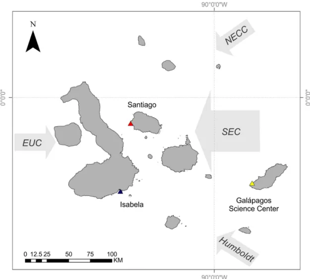
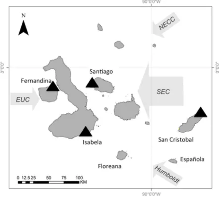
The Galápagos Islands are located 965 km off the coast of Ecuador and are centered at the confluence of several oceanographic currents leading to a high degree of variability in ocean temperature and phytoplankton biomass. The Equatorial Undercurrent runs from west to east across the Pacific Basin and drives major upwelling as it collides with the western islands, resulting in cold and nutrient-rich waters around these islands (Houvenaghel 1978, 1984). The cool Humbolt Current delivers nutrient-rich water to the southern edge of the archipelago (Kessler 2006). The northeast region of the archipelago is strongly influenced by the warm, nutrient-poor waters of the North Equatorial Countercurrent (NECC, or the Panama current) (Kessler 2006). Both of these currents contribute to the South Equatorial Current (SEC), a westward flowing current that strongly influences the central region of the archipelago (Houvenaghel 1984) (Fig. 1.1).
The dominant influence of the SEC changes seasonally, depending on the location of the Intertropical Convergence Zone (ITCZ) (Houvenaghel 1984). The ITCZ is north of the equator during the Garùa (fine mist) season (May to December), and the Humbolt Current is the major contributor to the SEC. During the wet season (December to May) the ITCZ shifts towards the south and the dominant influence to the SEC is the NECC. This results in fluctuating gradients of temperature and resource availability throughout the central archipelago.
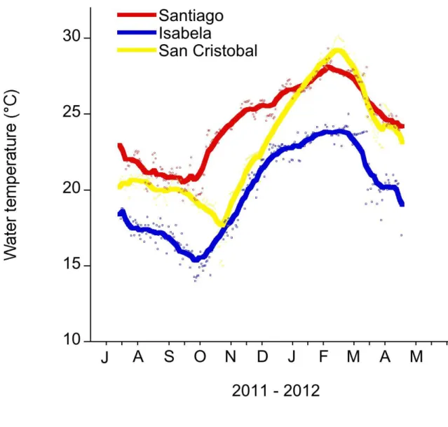
30°C in February 2012 and a low of 20°C in May 2012 (Fig. 1.2). This annual cycle is interrupted during ENSO events (Barber & Chavez 1983, Chavez et al. 1999).
During the warm ENSO phase (El Niño), the easterly trade winds weaken resulting in a deeper EUC thermocline, warmer waters and decreased upwelling. This results in low standing stock of primary producers in the euphotic zone (Pennington et al. 2006); and, ultimately marine consumer populations, such as seabirds, marine iguanas, and sea lions, decrease in abundance (Valle et al. 1987, Laurie & Brown 1990). In contrast, the cold ENSO phase (La Niña) occurs as the easterly trade winds strengthen, sea surface temperatures decrease, and upwelling intensifies resulting in higher standing stock of primary producers (Izumo et al. 2002). During La Niña, ocean temperature in the western islands can be as low as 11°C (Wellington et al. 2001).
In addition to regional-scale spatiotemporal variability in temperature and resource availability, the upwelling and downwelling of internal waves result in extreme and rapid temperature changes over smaller spatial and temporal scales (Witman & Smith 2003). For example, over a 53-week period on a rocky subtidal wall in the central archipelago at depths between 3-12m, 20 cold water events were recorded where temperature dropped by 3-9ºC over a 25 hr period (Witman & Smith 2003).
I tested the effect of temperature on the common subtidal herbivore Lytechinus
capable of converting algal turfs (brown filamentous turf, order Ectocarpales: Giffordia sp., Ectocarpus sp.) to urchin barrens in relatively short time periods, while Eucidaris does not have any detectable effect on the abundance of algal turfs (Irving & Witman 2009).
Ulva sp. was chosen as a food item for Lytechinus for several reasons: 1) Ulva sp. are one of the most abundant macroalgal species, along with turf, crustose coralline algae, and
Sargassum, in the Galápagos nearshore habitats (Vinueza et al. 2006, Vinueza 2009); 2) ephemeral species, like Ulva, are highly palatable for herbivores (Carpenter 1986); and 3) sea urchin fronts in the Galápagos appear to consume all macroalgal species except for brown species (e.g., Padina) (L. Carr personal observation) and damselfish turfs (Irving & Witman 2009).
Urchins and Ulva were haphazardly collected from the southern part of San Cristobal Island (89°36’41.85”W, 0°55’39.36”S), and were immediately transported to the laboratory in buckets filled with seawater. All urchins were collected from a depth of ~1.5 m. Study
organisms were maintained in culture tanks indoors at 23ºC (ambient sea water temperature) for two days prior to beginning water temperature adjustments. Assays were conducted in a shaded, outdoor facility at the joint UNC/USFQ Galápagos Science Center (San Cristobal Island,
Galápagos).
I conducted feeding rate assays in July 2012 to test the effect of two different
Ulva and urchins were placed in 4-L plastic container mesocosms and received a fresh supply of temperature-conditioned seawater every 12 hours. Temperature treatments were maintained with either Visi-Therm submersible individual heaters (Marineland, Blacksburg, Virginia, USA) or ice baths. Feeding assays were replicated twice (n = 5 replicates for each trial). Herbivore presence and absence treatments were randomly assigned in water tables. Each mesocosm was equipped with an iButton Thermochron datalogger (Dallas semiconductor, Dallas, Texas, USA) and water temperature was recorded every 5 minutes. Eight mesocosms were equipped with a HOBO Pendant temperature/light sensor (HOBO, Bourne, Massachusetts, USA) and relative light intensity was measured every 5 minutes.
Starting conditions for each mesocosm were 2.50 ± 0.004 g of wet mass Ulva tissue and either three urchins or no urchins (control to test for autogenic loss). The average test size for the urchins in the mesocosms was 3.55 ± 0.08 cm, which is representative of the green sea urchin populations in southern San Cristobal (n = 120 from two sites measured in May and June 2011: minimum 2.75 cm, maximum 5.8 cm. Mean ± 1 SE of 3.79 ± 0.61 cm).
Assays were terminated and final algal biomass was measured after 48 hrs (when ~ 50% of algal tissue was consumed (Tomas et al. 2011)). Biomass consumption was estimated as ([Hi
× Cf /Ci] – Hf), where Hi and Hf were the initial and final wet weights of algal tissue in the
presence of herbivores, and Ci and Cf were initial and final wet weights of the controls. Relative
light intensity levels did not vary between mesocosms and was 326.06 ± 19.7 lumens/ft2. These light levels are less than the average relative light levels at 1.5 m depth in the field (886.86 ± 74.07 lumens/ ft2), but are within the range of light conditions experienced throughout the tidal
Feeding rate assays were initially analyzed using a mixed model ANCOVA with one level of nesting. The analysis tested for one fixed effect (temperature treatment), covariate (urchin test size), and one random effect (temporal block). Consumption data were log transformed to meet the assumption of homogeneity of variances. The random effect was not significant (p = 0.183). Therefore, results were pooled and the random effect was dropped, for final analysis of treatment effects. All statistical analyses were performed in R (v. 2.15.2).
To estimate the temperature response of metabolic pathways (net photosynthesis and respiration), I measured oxygen production and consumption rates for Ulva and green urchins in 0.6L containers under conditions identical to the feeding rate assays. Initial and final oxygen concentrations were measured for Ulva (5 ± 0.08 g of leaf tissue) and paired blanks (seawater only) (n = 20 replicates) using a YSI-200 oxygen sensor (Yellow Springs Instruments, Yellow Springs, Ohio, USA). Samples of Ulva tissue (5 ± 0.08 g) were obtained by using three Ulva “rosettes” plucked from the substrate by the holdfast. Rosettes used were similar sizes and no cutting or tearing was necessary. After the initial measurement, aquaria were covered with plastic to minimize oxygen exchange with the air and left for 2 hrs. Net photosynthesis rates were estimated by subtracting measurements of dark oxygen consumption from light oxygen production.
development of strong oxygen and temperature gradients. The chamber was placed into a water bath to maintain temperature treatments. An individual urchin was then placed into the chamber and oxygen concentrations were measured every five minutes for one hour at each temperature treatment (14°C and 28°C). Trials were repeated for 11 urchins. The mean weight specific oxygen consumption rate (Q, mg O2 kg-1 h-1) was calculated with the equation of Karamushko
and Christiansen (2002):
Q = (C0 – Ct)V/WT
C0 and Ct are the initial and final oxygen concentration (mg O2 l-1), respectively. V is the volume
(l) of the chamber minus the test urchin volume (test urchin volume was estimated from their biomass). W is the biomass of the urchin in kg. T is the measurement time in hours.
Oxygen consumption and production test were analyzed with a t test on change in O2. All
statistical analyses were conducted using R (version 2.15.2).
Results
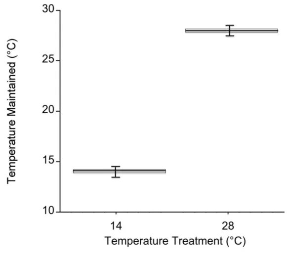
Temperatures in the cold mesocosms were maintained at 14.01 ± 0.08ºC and 14.03 ± 0.07ºC for trials 1 and 2, respectively. Warm mesocosms for trials 1 and 2 were 28.06 ± 0.09ºC and 28.00 ± 0.04ºC, respectively. The range of temperatures maintained across both trials was 13.54 – 14.47ºC for the cold treatment and 27.56 – 28.5ºC for the warm treatment (Fig. 1.3). Green urchin consumption was 46% higher at the warmer temperature (p < 0.0001) (Fig. 1.4A). Urchin test size was not a significant covariate (p = 0.87).
at 28ºC, 3.24 ± 0.13 g O2•g tissue-1•hr-1; p = 0.004). Oxygen production was also greater at 28ºC
(at 14ºC, 3.88 ± 0.09 g O2•g tissue-1•hr-1; at 28ºC, 4.74 ± 0.15 g O2•g tissue-1•hr-1; p = 0.01).
However, net photosynthesis rates did not vary with temperature (p = 0.45, Fig 4C).
Discussion
Consistent with the predictions based on metabolic theory and a growing body of
literature, my results indicated that sublethal warming significantly increases the strength of top-down effects. Specifically, I found a 14°C increase in temperature resulted in a 46% increase in grazing rate and lower standing plant biomass. Similar results have been found in other marine systems (O’Connor 2009: with herbivores there was a nearly 100% decrease in algal net growth at high temperatures compared to growth at low temperatures with or without herbivores) and grasslands (Barton et al. 2009: warming of 1°C increased the strength of top-down indirect effects on grasses and forbs by 30-40%).
One limitation of my study was that the urchins and algae might have acclimated to the ~5°C temperature change had I warmed the treatment tanks more slowly or maintained the experiment for longer. Thus, it is difficult to extrapolate to how slower or longer-term changes in temperature will affect urchin-algal interactions and, consequently, larger spatial scale
While there was a significant temperature effect on consumer metabolism and feeding rates, there was not a significant temperature effect on algal photosynthesis rates following the 4-day acclimation period in this study. It is possible that this was because light, nutrients, carbon dioxide, or some other resource was limiting and thus warming could not stimulate
photosynthesis. Further, the positive effect of increased temperature on algal photosynthetic rate can be reduced or reversed at sub-saturating light levels because warming can increase the light level needed to reach the compensation point (Davison 1991). Light conditions in the
experiment were within the range of light levels in the nearshore habitats in the Galápagos (Table 1) and further, most populations of subtidal algae are subject to subsaturating light
conditions (Davison 1991); therefore the experimental conditions likely reflect algal performance in the field. My results are consistent with O’Connor (2009) which found no temperature effect for Sargassum with a 4°C temperature change.
At the upper range of species’ thermal tolerances metabolism and consumption are predicted to scale differently and metabolic demands should outpace increased grazing intensity (Rall et al. 2010). Lemoine and Burkepile (2012) found Lytechinus variegatus consumption and metabolism scaled differently at temperatures beyond 29°C, a 9°C increase from the starting temperature treatment (20°C). Ultimately, urchin ingestion efficiency was decreased at the higher temperature, resulting in possible reduced consumer fitness. Because shallow subtidal temperatures around San Cristobal reach 30°C, future work should focus on understanding Lytechinus metabolism/consumption ratios at the highest temperatures in the Galápagos and the implications for species interactions and the strength of top-down effects under these conditions.
spatial scales, and various environmental conditions (i.e., different seasons, ENSO cycles, varying light intensities, etc.) and with different algal species.
The absence of macroalgae in intertidal and shallow subtidal habitats during warm periods (e.g., El Niño) in the Galápagos Islands is generally attributed to the decreased strength of bottom-up forcing (i.e., upwelling) and subsequent lack of nutrients (Vinueza et al. 2006). However, temperature stress (i.e., desiccation) does play a minor role in regulating intertidal algal biomass in the Galápagos (Vinueza 2009). Therefore, future work should focus on understanding the constraints of physical stress on macroalgal growth in the Galápagos Islands, as stress is known to alter the relative importance of bottom-up and top-down effects (Thompson et al. 2004).
Low macroalgal biomass in warm seasons and years could also be due in part to increased grazing intensity due to higher temperature (e.g., O’Connor et al. 2009). Both
mechanisms could be operating (i.e., changes in top-down and bottom-up control), although the relative strength of these mechanisms in influencing large-scale ecological patterns in upwelling systems is unknown. In freshwater pond systems, Kratina et al. (2012) found a negative
Table 1.1 Natural variation in algal cover, temperature and urchin density in shallow subtial habitats in the Galapagos Islands.
Sites were surveyed in June 2010 and July 2012. Site codes: LL = La Loberia (San Cristobal, SC), LT = Las Tijeretas (SC), PP = Punta Pitt (SC), CD = Cabo Douglas (Fernandina, FE), PE = Punta Espinosa (FE). Values represent means ± SE (n = 25 quadrats for urchin density and algal cover). Any other urchin species (e.g., Tripneustes) were present at densities less than 0.3m-2 in
all quadrats. Temperature was estimated with both in situ temperature loggers and satellite data (AQUA Modis) for the 30-day period prior to sampling, SE < 0.07 for all sampling points. Light intensity was measured using HOBO Light/Temperature Pendants before and during the
experimental duration.
2010 2012
Site LL LT PP CD LL LT PE
Ulva cover (%) 9.7 ± 3.3 58.4 ± 3.5 2.9 ± 0.4 36.3 ± 5.1 7.8 ± 2.1 28.9 ± 2.7 23.4 ± 1.5 Eucidaris density (m-2) 4.8 ± 1.3 1.6 ± 0.7 1.6 ± 0.2 8.4 ± 2.4 6 ± 1.9 2.1 ± 0.4 3.2 ± 1.3 Lytechinus density (m-2) 10.2 ± 2.6 11.8 ± 1.8 11.2 ± 1.9 1.2 ± 0.7 14.9 ± 2 13.2 ± 1.6 17.6 ± 4.5 Temperature (°C) 24.8 23.7 20.8 11.4 25.3 23.2 17.8
Light Intensity Range
Figure 1.1 Map of Galapagos Archipelago and the surrounding currents.
Figure 1.2Daily water temperature (mean) measured in the shallow subtidal (< 5m) at Santiago, Isabela and San Cristobal
The Galapagos Science Center is on San Cristobal. Water temperature measurements were recorded every 30 mins with a HOBO temp logger. The smoothing curve was done in
Figure 1.3 Mesocosm temperature values during both experiments.
Temperature in each mesocosm (n = 20 per temperature) was recorded every 5 mins. with an iButton Thermochron datalogger (Dallas semiconductor, Dallas, Texas, USA). The box
Figure 1.4 Temperature effects on urchin grazing rates, metabolism and algal photosynthesis.
CHAPTER 2: TEMPERATURE INFLUENCES HERBIVORY ACROSS A REGIONAL-SCALE TEMPERATURE GRADIENT IN THE GALAPAGOS ISLANDS, ECUADOR
Introduction
Understanding how the abiotic environment influences species interactions has long been a fundamental goal of ecological research (e.g., Park 1954, Dunson & Travis 1991, Brown et al. 2004). For example, environmental temperature can influence the direction and magnitude of species interactions (Davison 1987, O'Connor 2009). Stressful temperatures can modify the physiological ecology of organisms, resulting in changes to the outcomes of species interactions and initiating changes that propagate to community-level patterns (Menge & Sutherland 1987). Recently, ecological theory and empirical studies have examined how non-stressful (non-lethal) temperatures influence species interactions via predictable effects on individual metabolic function (Davison 1987, Brown et al. 2004).
relative to photosynthesis and thus, consumption might be stronger at warmer (sublethal) temperature compared to production (Allen et al. 2005).
A growing body of empirical work does demonstrate consumption increases relative to production with (non-stressful) warmer temperatures (e.g., O’Connor 2009, O’Connor et al. 2009, Hoekman 2010, Kratina et al. 2012, Shurin et al. 2012, Carr & Bruno 2013). A wide range of lab-based experiments (i.e., environmental chambers) and mesocosm studies conducted in freshwater, marine and terrestrial systems found sublethal warming can increase per capita grazing rate and the effect of herbivores on plant biomass, ultimately, resulting in less standing plant biomass at higher temperatures (e.g., O'Connor 2009, Hoekman 2010, Kratina et al. 2012, Sentis et al. 2012, Carr & Bruno 2013). As the strength of herbivore-plant interactions can determine primary producer abundance in a community (Lubchenco & Gaines 1981, Paine 1992, Burkepile & Hay 2006), the temperature dependence of herbivore-plant interactions could translate to alterations in larger-scale ecological patterns, such as primary producer biomass, composition, and distribution.
latitude (e.g., phenotypic variation, physical oceanographic features, species composition, etc.) and could influence in situ feeding rates.
We employed a comparative-experimental design (Menge 1991) along the same latitude across a natural gradient in temperature (via upwelling and oceanographic currents) to quantify its influence on the effects of subtidal benthic and mobile herbivores on algal biomass in the Galápagos Islands. Specifically, we utilized two aspects of thermal variability across the
Archipelago: inter-annual (warm and cold season) and spatial (warm and cold areas). Further, to examine whether the temperature-dependence of grazing rates could affect community-level patterns (i.e., standing algal biomass in this system), we also conducted a longer-term field exclusion experiment at one upwelling region.
This system is ideal for examining the effects of temperature on species interactions because the Archipelago is centered at the convergence of several different oceanographic currents (tropical, subtropical and upwelled water), resulting in enormous spatiotemporal
variation in water temperature (11°C - 31°C) (Houvenaghel 1984, Schaeffer et al. 2008, Witman et al. 2010). Further, while community composition differs across the Archipelago due to upwelling intensity, there is a suite of organisms that are present at all the sites throughout the year. Thus, this system is a subtidal analogue of the rocky intertidal zone; a continental scale thermal gradient compressed into tens of kilometers and relatively short time scales.
Methods
Archipelago. The Equatorial Undercurrent (EUC) drives major upwelling as it collides with the western islands, resulting in cold and nutrient-rich waters around Fernandina (Houvenaghel 1984). The study site was located at Punta Espinosa, on the northeastern point of the island (Fig. 2.1), (0°16’06.88”S, 91°26’50.49”W). Isabela is also located in the western region; and assays were conducted on the southern edge of the island, at Túnel del Estero (0°57’39.46”S,
90°59’26.28”W). This region is influenced by the EUC and the cool (and nutrient-rich) Humboldt Current from the south, therefore, this region is also considered an upwelling zone (Houvenaghel 1984, Schaeffer et al. 2008) (Fig. 2.1). Santiago is a northern island, located in the central region of the Archipelago. The study site, Puerto Egas (0°15’13.58”S,
90°52’05.18”W), is located on the northwest side of the island. And influenced by the South Equatorial Current (SEC; a westward flowing current that strongly influences the central region of the Archipelago), the North Equatorial Countercurrent (NECC, a warm and nutrient-poor current) and EUC meanderings, resulting in high productivity, yet warmer waters (Houvenaghel 1984, Schaeffer et al. 2008) (Fig. 2.1). San Cristobal is the easternmost island in the
Archipelago. Grazing assays were conducted at Punta Pitt (0°42’38.93”S, 89°15’02.87”W), located on the northeastern point of the island, and influenced by the SEC, Humboldt Current, and the NECC (Houvenaghel 1984, Wellington et al. 2001, Schaeffer et al. 2008). In general, this site has depressed nutrient loads and warmer waters relative to the other sites, as it is north of the upwelling region off San Cristobal (Schaeffer et al. 2008).
average SST usually occurring in August or September. The maximum average SST usually occurs in February and March, when the dominant influence to the SEC is the NECC.
In the Galápagos shallow subtidal, macroalgae are generally the dominant sessile group
and sea urchins are the most significant invertebrate grazer guild (Irving & Witman 2009, Brandt, Witman & Chiriboga 2012). At high densities, sea urchins can convert macroalgal assemblages to urchin barrens or pavements of encrusting algae (Edgar et al. 2010). The two most common sea urchins in rocky subtidal habitats at depths between 1 and 5 m are Lytechinus
semituberculatus (green sea urchin)and Eucidaris galapagensis (slate pencil sea urchin).
Lytechinus is capable of converting algal turfs to urchin barrens in relatively short time periods,
while Eucidaris does not have any detectable effect on algal turf abundance (Irving & Witman 2009). Other important grazers include fishes (razor surgeonfishes; Prionurus laticlavius, blue chin parrotfish; Scarus ghobban), sea turtles and marine iguanas.
Natural herbivore densities and benthic community composition were assessed at each
site and during both time periods (Table 2.1). We quantified benthic community composition,
fish community composition, biomass and density, and urchin identity and abundance along five
30m transects placed parallel to shore at ~3-4m depth.
Along each transect,five photoquadrats were placed adjacent to the transect line at fixed
intervals, totaling 25 photquadrats per site. Each photograph captured an area of 0.42 m2. One
hundred points were placed over each photograph in a stratified random design. Image analysis
Divers conducted visual fish censuses along 30 x 2m belt transects by recording the
species-level identity and length of each fish. Fish length estimates were converted to fish
biomass estimates using published length-biomass relationships (Froese & Pauly 2013). Urchin
identity and abundance was determined by counting all urchins along 30 x 1m belt transects.
To examine the effect of temperature on grazing rates of Ulva (chosen as a food item because it is one of the most abundant macroalgal species in nearshore habitats (Vinueza et al. 2006, Table 2.1) and is highly palatable (Carpenter 1986), we repeated the same grazing rate assay in situ at four sites and two time periods (warm and cold season) in 2013. The total temperature range was 19.7 – 29.5°C, with the warm (Feb/Mar 2013) and cold season (Sept/Oct 2013) temperatures ranging from 24.4 – 29.5°C and 19.7 – 24.7°C, respectively.
Three different cage types were deployed: closed cages with Lytechinus absent (control), closed cages with Lytechinus present, and open cages (no sides or top) (n = 10 for each cage type). Open cages were used to assess the temperature effect on natural grazing conditions at each site and time period. Lytechinus and Ulva were haphazardly collected at each site from a depth of ~2m. The average test size for the urchins placed in cages across all sites and both time periods was 3.82 ± 0.09 cm, which is representative of the green sea urchin populations across the Archipelago (see Table 1 for urchin test sizes in cages for each site and time period).
Urchins were then placed in cylindrical vexar cages at a depth of ~3 – 5m and starved for ~ 30 h. Cages were constructed using plastic vexar looped in cylinders with a diameter of 30cm, 15cm height, and a mesh size of 2.5cm. Chain was placed on the substrate at ~3 – 5m depth and cages were attached to the chain via metal fasteners. Treatments were randomly assigned along the chain. Water temperature was measured and recorded every 5 minutes with a HOBO
Initially, each cage contained 5.00 ± 0.06 g of wet mass Ulva tissue and either three urchins or no urchins (control to test for autogenic loss). Ulva was strung onto bead wire and then was attached to the vexar. The urchin densities used in the cages are representative of natural urchin densities at these sites (Table 2.1). Scaled for comparison, we used 21 green urchins per 0.5m2, andthe range of green urchin densities found at the sites was between 11 and 39 per 0.5m2. Assays were terminated and final algal biomass was measured after 24 h, as over
~50% of algal tissue was consumed (Tomas et al. 2011). Biomass consumption was estimated as ([Hi × Cf /Ci] – Hf) = FB, where Hi and Hf were the initial and final wet weights of algal tissue in
the presence of herbivores, and Ci and Cf were initial and final wet weights of the controls.
Percent consumed (or grazing rate) was determined from FB/Cf.
25cm, 12cm height, and a mesh size of 2.5cm. After construction, boulders were haphazardly placed at a depth of ~5m. Boulders were sampled 12 weeks later, and all macroalgae was collected from the cages/plots. Macroalgae collected from each cage was recorded to genus, spun in a salad spinner for 60 revolutions, and then weighed.
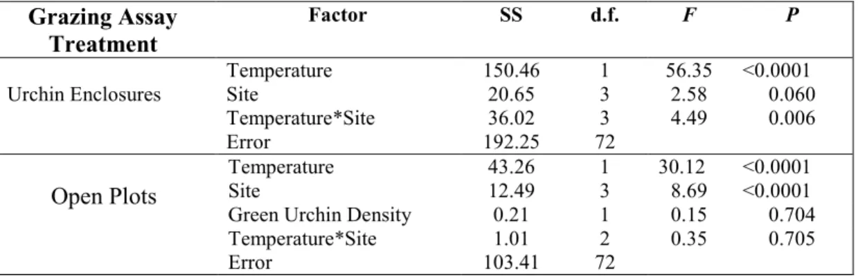
For the grazing assays, we conducted 1) a two-factor analysis of variance (ANOVA) on urchin grazing rate, with site and temperature as fixed factors, and 2) a two-factor analysis (ANCOVA) on the open plot grazing rate, with site and temperature as fixed factors, and green urchin density as a covariate. A logistic (logit) transformation was applied to the grazing rates (Lesaffre et al. 2006). For the field exclusion experiment, we compared treatment effects on final algal biomass using a one-way analysis of variance (ANOVA). The field exclusion analysis was followed with Tukey’s HSD post-hoc tests. All analyses were run in R v. 3.0.3 (R Development Core Team 2014).
Results
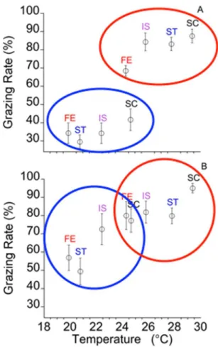
In the urchin-only treatment, urchins consumed 40% more Ulva at warmer temperatures than cooler temperatures (Table 2.2, Fig. 2.2A). There was not a significant site effect on grazing rates. However, there was a significant site x temperature interaction (Table 2.2, Fig. 2.2A), as grazing rates at San Cristobal and Fernandina were different at the same temperature (Fig. 2.2A).
In the open plots, temperature and site were significant factors influencing grazing rates (Table 2.2, Fig. 2.2B). Green urchin density was not a significant covariate (Table 2.2). And there was not a significant site x temperature interaction. In the open plots, grazers (including urchins and fishes) consumed 21% more Ulva at in the warm season relative to the cold season.
Final algal biomass differed significantly between treatments (Table 2.3, Fig. 2.3, post-hoc Tukey HSD tests). Overall, there was 90% more algal biomass in the full exclusion plots relative to the open plots. There was 48% and 54% less algal biomass in the mobile and benthic herbivore treatments, respectively, relative to the full exclusion plots (Fig. 2.3). Although, the final algal biomass in the mobile herbivore treatments compared to the benthic herbivore treatments were not different from each other (post-hoc Tukey HSD tests). The dominant algal functional group present in the treatments was green sheet-like algae (Ulva spp.), and the percent composition of Ulva spp. were similar across treatments: 83.3%, 81.7%, 77.1%, and 79.2%, open plots, benthic herbivores, mobile herbivores, and full exclusions respectively. Red filamentous algae (Ceramium spp., Centroceras spp. and Polysiphonia spp.) were present with the following percent composition: 16.9%, 13.5%, 22.9%, and 18.3%, open plots, benthic herbivores, mobile herbivores, and full exclusions respectively. The least common algal functional group present was red corticated algae (Hypnea spp.): 0%, 4.8%, 0%, and 2.5%, open plots, benthic herbivores, mobile herbivores, and full exclusions respectively.
Consistent with predictions based on metabolic theory and a growing body of evidence from empirical studies conducted in environmental chambers, our results indicated that sublethal warming significantly increases the strength of herbivory across a natural, in situ, mesoscale temperature gradient. Overall, we found that a ~10°C change in temperature resulted in 40% and 21% increases in grazing rate for urchin-only and open plots in our grazing assays, respectively. These results are consistent with a similar study conducted in mesocosms on San Cristobal Island that found a 14°C temperature increase resulted in a 46% increase in L. semituberculatus grazing rates (Carr & Bruno 2013). Further, results from our field exclusion experiment found in the absence of herbivores, algal biomass increased by almost 90%. Also, a recent meta-analysis on herbivore grazing rates found increasing ambient temperature resulted in higher per capita and community level grazing rates. Therefore, our results coupled with findings from meta-analyses, such as Hillebrand et al. (2009), suggest herbivores could have a strong effect on algal biomass even in nearshore upwelling systems.
Further, in support of several recent studies (Shurin et al. 2012; Sentis et al. 2012; Dell et al. 2013), we found the temperature effect on grazers was context-dependent. Specifically, our results are consistent with local acclimatization, in the urchin-only treatment; urchins consumed different amounts of Ulva at the same temperature at different sites (significant site x
temperature during the warm season at Fernandina was low relative to the rest of the
Archipelago, it was warm relative to the average water temperature in this region (21.6°C from Feb – Dec 2013, Carr unpublished data; and 22.1°C from Jan 2006 – Jan 2009, Vinueza et al. 2014).
That thermal history influences acclimatization is well documented (Roberts 1957, Hutchison 1976, Helmuth 2002). For example, a recent study (Marshall & McQuaid 2010) found that the relationship between metabolic rate and temperature depends on the temperature range experienced by the organism. However, less is known about other biological responses of organisms in response to thermal history, and our findings suggest this mechanism may be important for consumption rates. However, there could be other alternative explanations for the discrepancy in grazing rates at different sites at the same temperature due to site-specific
differences. For example, current characteristics, wave exposure, and other physical attributes could vary among sites and influence plant growth, biomass, and even grazing (Dayton 1985, Irving & Witman 2009). Therefore, future studies should focus on isolating the direct
mechanism of variation in biological responses (such as consumption rates) at similar temperatures at regional scales.
density did differ between sites and time periods (Table 2.1), this was not a significant factor influencing grazing rates. Therefore, an increase in grazing rates with temperature was not a function of changes in green urchin density. These open plots tested the generality of
temperature effects on herbivore-algal interactions under more natural conditions. We expected to see higher variance in these assay plots, given the among-plot and -site variance in grazer communities (composition and density, Table 2.1). Nonetheless, more Ulva was consumed in the open plots at warmer temperatures even when we did not control for variance in the grazer community (Fig. 2.2B), suggesting the observed effects are general and relatively strong.
At the upper range of species’ thermal tolerances, metabolism and consumption are predicted to scale differently and metabolic demands should outpace increased grazing intensity (Rall et al. 2009), leading to decreased strength of top-down effects (Lemoine & Burkepile 2012). However, at the sites with the two warmest temperatures (28°C and 29.5°C), the shallow subtidal temperatures often reach 30°C during the warm season (Carr & Bruno 2013); therefore, the temperatures in these assays were representative of the natural temperature regime.
The utilization of a macroecological approach, such as a comparative-experimental design, to examine the tempesrature dependence of herbivore-algal interactions across relatively large spatial and temporal scales, can provide insight into the possible effects on larger-scale ecological patterns (i.e., primary producer composition and biomass). For example,
Lytechinus is locally abundant, the higher grazing rates at warm sites and during warmer seasons and years (e.g., El Niño) may increase the prevalence of urchin barrens or alter algal community composition due to the increased relative strength of herbivory, despite an increase in primary productivity.
Because this study focused on Ulva spp., we cannot extrapolate to how temperature would affect other algal-urchin interactions. Nonetheless, Ulva spp. is by far the most abundant macroalgal species in intertidal and shallow subtidal habitats (Vinueza et al. 2006, Carr & Bruno 2013, Vinueza et al. 2014, Table 2.1). And further, Ulva spp. was the most abundant algal species present in the field exclusion experiment (Fig. 2.3). Notably, this experiment lasted for 12 weeks, however; herbivore exclusion experiments in the Galápagos intertidal conducted over months and years have found ephemeral species (e.g., Ulva spp.) are one of the dominant macroalgal species, along with competitively dominant species, like coralline algae (Vinueza et al. 2006, 2014). Therefore, results from both our (and others) field exclusion experiment(s) and field surveys are consistent: Ulva spp. is a dominant benthic space occupier in the Galápagos shallow subtidal and thus, changes in herbivore-Ulva interactions could strongly influence algal community biomass and composition across the Archipelago.
Our results are also consistent with other studies conducted in the intertidal across varying upwelling conditions that suggest herbivore effects on algal community structure can also be driven by changes in the responses of less palatable, corticated algae (Nielsen &
between the intertidal and subtidal. For example, some species of parrotfish exhibit a strong preference for Hypnea spp. and Gracilaria spp. (Mantyka & Bellwood 2007). Our results support this finding as Hypnea spp. were absent from the plots most likely to be visited by parrotfishes, (i.e., open plots and mobile herbivore treatments).
Although Vinueza et al. (2006, 2014), working in intertidal habitats in the Galápagos (our study was conducted in the shallow subtidal) attributed greater algal biomass among sites to local nutrient concentration via spatiotemporal variation upwelling intensity, nutrient concentration was not quantified or manipulated. And further, Schaeffer et al. (2008) measured nitrate availability and temperature across the Archipelago at four different times and at 70 stations, generating 280 sampling points, and did not find the expected negative relationship between nutrient availability and temperature (R2 = 0.002), unlike other studies in temperate upwelling systems (e.g., Nielsen & Navarrete 2004). Therefore, it is unlikely that the relationship between temperature and standing algal biomass and growth in the Galápagos can be solely attributed to nitrate availability.
Moreover, the results from Vinueza et al. (2006, 2014) were also consistent with temperature-dependent grazing as temperature was positively related to grazing rate (and generally declined during upwelling). However, the potential role of temperature was not
explicitly tested. Favoring a bottom-up explanation over the possibility of temperature-mediated top-down effects is a nearly universal phenomenon in studies of the role of algal-herbivore interactions in upwelling systems (e.g., Menge & Branch 2001, Nielsen & Navarette 2004). Furthermore, like Vinueza et al. (2006, 2014), the norm is to not measure or even manipulate nutrient availability, but rather to use upwelling (and chlorophyll a) as a natural (nutrient
These mensurative studies have led to the paradigm that upwelling systems are largely bottom-up controlled. Yet our field exclusion experiment clearly demonstrates the very large role of grazers in controlling standing algal biomass during the upwelling season in an upwelling region, suggesting top-down effects are also important in this system, even with temperature induced changes in herbivory (i.e., upwelling and cold periods can dampen the strength of grazing).
Recent evidence from microcosms and ecological theory suggests herbivore-plant interactions in upwelling systems could be disproportionately affected with warming
temperatures (Smith 2008, O'Connor et al. 2009). For example, O’Connor et al. (2009) found that in nutrient-limited regions, food webs may be more resilient to warming because consumer production and biomass is limited by resource availability. In contrast, in upwelling or well-mixed systems, where nutrient availability is high, small levels of warming can lead to stronger consumer control of primary producer biomass and ultimately, alter food web structure
(O'Connor et al. 2009). In further support, results from a global meta-analysis found that even with the expectation of more intense grazing in the tropics and a positive relationship between herbivore feeding rates and temperature, the exclusion of herbivores did not result in higher standing algal biomass relative to temperate regions (Poore et al. 2012). Thus, these results suggest stratification of the water column in tropical waters maintains lower nutrient availability (Poore et al. 2012) and therefore, tropical systems are more constrained by limited nutrient availability relative to temperate regions, where nutrient availability is high, and thus,
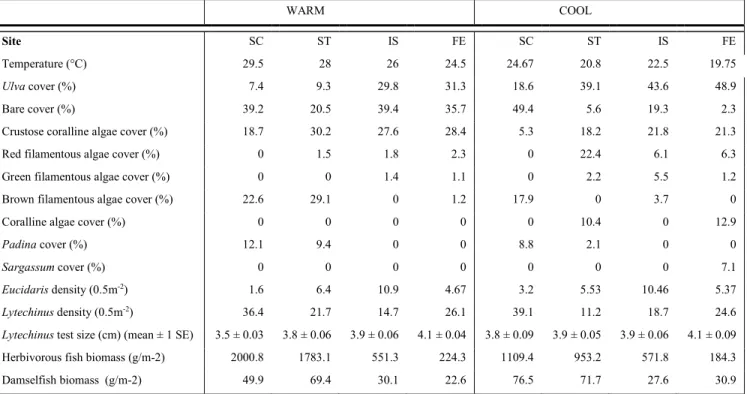
Table 2.1. Natural variation in site attributes.
Site codes: SC = San Cristobal, ST = Santiago, IS = Isabela, FE = Fernandina. Values represent means (n = 25 quadrats for algal cover). Urchin density and fish biomass was determined as described in Methods section.
WARM COOL
Site SC ST IS FE SC ST IS FE
Temperature (°C) 29.5 28 26 24.5 24.67 20.8 22.5 19.75
Ulva cover (%) 7.4 9.3 29.8 31.3 18.6 39.1 43.6 48.9
Bare cover (%) 39.2 20.5 39.4 35.7 49.4 5.6 19.3 2.3
Crustose coralline algae cover (%) 18.7 30.2 27.6 28.4 5.3 18.2 21.8 21.3
Red filamentous algae cover (%) 0 1.5 1.8 2.3 0 22.4 6.1 6.3
Green filamentous algae cover (%) 0 0 1.4 1.1 0 2.2 5.5 1.2
Brown filamentous algae cover (%) 22.6 29.1 0 1.2 17.9 0 3.7 0
Coralline algae cover (%) 0 0 0 0 0 10.4 0 12.9
Padina cover (%) 12.1 9.4 0 0 8.8 2.1 0 0
Sargassum cover (%) 0 0 0 0 0 0 0 7.1
Eucidaris density (0.5m-2) 1.6 6.4 10.9 4.67 3.2 5.53 10.46 5.37
Lytechinus density (0.5m-2) 36.4 21.7 14.7 26.1 39.1 11.2 18.7 24.6
Lytechinus test size (cm) (mean ± 1 SE) 3.5 ± 0.03 3.8 ± 0.06 3.9 ± 0.06 4.1 ± 0.04 3.8 ± 0.09 3.9 ± 0.05 3.9 ± 0.06 4.1 ± 0.09 Herbivorous fish biomass (g/m-2) 2000.8 1783.1 551.3 224.3 1109.4 953.2 571.8 184.3
Table 2.2 Two-factor ANOVA and ANCOVA on control-corrected grazing rates.
Grazing Assay Treatment
Factor SS d.f. F P
Urchin Enclosures
Temperature 150.46 1 56.35 <0.0001
Site 20.65 3 2.58 0.060
Temperature*Site 36.02 3 4.49 0.006
Error 192.25 72
Open Plots
Temperature 43.26 1 30.12 <0.0001
Site 12.49 3 8.69 <0.0001
Green Urchin Density 0.21 1 0.15 0.704 Temperature*Site 1.01 2 0.35 0.705
Table 2.3. One-factor ANOVA on final algal biomass.
Factor SS d.f. F P
Treatment 723.5 3 32.1 <0.0001
Figure 2.1.Map of the Galápagos Islands and the surrounding currents.
Figure 2.2. Temperature effects on A) urchin and B) mobile and benthic herbivore consumption of Ulva.
Biomass consumption was estimated as ([Hi × Cf /Ci] – Hf) = FB, where Hi and Hf were the initial
and final wet weights of algal tissue in the presence of herbivores, and Ci and Cf were initial and
final wet weights of the controls, FB = amount consumed. Percent consumed was determined
from FB/Cf. Letters above error bars correspond to island (site) name. FE = Fernandina, ST =
Figure 2.3. Herbivore effects on algal biomass.
CHAPTER 3: SPATIOTEMPORAL VARIATION IN THERMAL REGIMES AND CONSUMER ASSEMBLAGES INFLUENCES SUBTIDAL BENTHIC COMMUNITIES
ACROSS THE GALAPAGOS ISLANDS
Introduction
At the interface of marine ecology and oceanography, a substantial body of work has identified some of the main physical oceanographic processes that can regulate nearshore benthic communities (e.g., Menge 1976, Menge and Lubchenco 1981, Bustamante et al. 1995, Connolly and Roughgarden 1998, Dayton et al. 1999, Roughgarden 2006). There are three major benthic-pelagic pathways, nutrient transport and deposition, larval recruitment and temperature mediated metabolism (Witman and Dayton 2001). These processes can drive benthic-pelagic coupling via physical linkages between these two environments. All three pathways can be modulated by changes in the frequency, duration, and magnitude of upwelling, or the wind-driven
oceanographic process of cool, nutrient-rich subsurface currents replacing warmer, nutrient-poor surface currents.
such as growth, reproduction, and consumption, in predictable ways. Specifically, warmer (cooler) water increases (decreases) metabolic rates (Brown et al. 2004). And while upwelled water is nutrient rich, it is also cooler. Metabolic theory coupled with a growing number of empirical studies suggest temperature can decrease metabolic rates in upwelling systems with consequent effects on community dynamics (Smith 2008, O’Connor et al. 2009, Carr and Bruno 2013).
In upwelling systems, macroalgal assemblages are an important part of the subtidal benthic community. Macroalgae-associated consumers (fishes and other grazers) can drive changes in macroalgal biomass and community composition and distribution (Schiel and Foster 1986, Chapman and Johnson 1990, Sala and Boudouresque 1997). For example, exclusion of an herbivorous fish in a temperate rocky reef system in Chile was consistent with changes in
macroalgal community composition (increased abundance of green versus red foliose
macroalgae) (Ojeda et al. 1999). At high densities, invertebrate grazers, such as sea urchins, can convert macroalgal assemblages to urchin barrens or pavements with bare space and encrusting algae (Chapman and Johnson 1990, Ruttenberg 2001, Edgar et al. 2010).
Numerous studies have examined the relative strength of physical forcing and plant-herbivore interactions on intertidal benthic community structure across varying oceanographic patterns in upwelling systems (e.g., Bustamante et al. 1995, Bustamante and Branch 1996, Menge et al. 1999, Broitman et al. 2001, Menge et al. 2003, Nielsen and Navarrete 2004,
Although the Galápagos Islands are situated on the equator, due to the strong upwelling signal across the Archipelago, the biological community is in many ways more temperate than tropical (Edgar et al. 2004, Vinueza et al. 2006, Witman et al. 2010, Brandt et al. 2012, Carr and Bruno 2013, Vinueza et al. 2014). Recent studies of benthic-pelagic coupling in the Galápagos have focused on how upwelling influences 1) propagule transfers within and among subtidal rock-wall habitats (Witman et al. 2010) and 2) how bottom-up forcing of nutrients influences intertidal benthic communities (Vinueza et al. 2006, 2014).
Due to spatial, daily, seasonal, and annual changes in oceanographic currents, the nearshore systems of the Galápagos Islands experience tremendous variation in ocean
temperature (11 – 31°C) (Houvenaghel 1984, Schaeffer et al. 2008, Witman et al. 2010). The main foundation species in the shallow nearshore (< 3m) benthic community is macroalgae (e.g., Ulva spp., Sargassum spp.) (Vinueza et al. 2006, Carr and Bruno 2013, Carr et al. in review). And similar to many other temperate systems, sea urchins are the most important invertebrate grazer guild in the Galápagos (Irving and Witman 2009, Brandt et al. 2012), although other important grazers include fishes (razor surgeonfish, blue chin parrotfish), sea turtles and marine iguanas.
Previous work in the Galápagos on spatial and temporal variation in macroalgal
assemblages has focused on intertidal sites (e.g., Vinueza et al. 2006, 2014). And specifically, how macroalgal communities vary at a couple of sites over time across gradients in
oceanographic conditions and grazing pressure. In the shallow subtidal, past experimental work demonstrated that identity (and not diversity) of sea urchins drives changes in benthic
higher at warmer relative to cooler temperatures (Carr & Bruno 2013, Carr et al. in review). However, little is known about the spatiotemporal dynamics of macroalgal communities of the shallow subtidal habitats across the Galápagos Archipelago. Such information is important because it lays the foundation for exploring the relationship between benthic community
structure and biotic and abiotic processes that generate these patterns (Underwood et al. 2000). Our objectives were 1) to provide a comprehensive description of the shallow subtidal benthic community patterns across sites, seasons and years in the Galápagos Archipelago, 2) to examine how large-scale physical forcing, via natural temperature gradients, changes benthic community dynamics, and 3) to investigate the relative effects of local scale interactions and large-scale processes on benthic community organization.
Methods
The Galápagos Islands straddle the equator 965 km off the coast of Ecuador in the
Eastern Pacific Ocean at the center of several different oceanographic currents. The Equatorial
Undercurrent (EUC) is an eastward flowing subsurface current that drives major upwelling as it
collides with underwater seamounts near the western islands resulting in cold and nutrient-rich
water around these islands (Houvenaghel 1978, 1984). The southern region of the archipelago is strongly influenced by the cool, and nutrient-rich waters of the Humboldt (or Peru) Current
(Kessler 2006). The North Equatorial Countercurrent (NECC, or the Panama current) delivers warm, and nutrient-poor water to the northeast region (Kessler 2006). Both the Humboldt Current and the NECC contribute to the westward flowing South Equatorial Current (SEC),
maximum average sea surface temperature (SST) usually occurs in February and March. In
contrast, the minimum average SST usually occurs in August or September, when the dominant
influence to the SEC is the Humboldt Current. However, ENSO events can disrupt the seasonal
cycle (Barber and Chavez 1983, Chavez et al. 1999).
The easterly trade winds weaken during El Niño events (or the warm ENSO phase
defined by the NOAA Climate Prediction Center as a SST anomaly of +0.5°C on the Oceanic
Niño index for a minimum of five consecutive seasons), resulting in a deeper EUC thermocline,
warmer waters, and ultimately, decreased upwelling throughout the Archipelago. Generally, this
results in low primary producer standing stock in the euphotic zone (Pennington et al. 2006). In contrast, during La Niña, (the cold ENSO phase, a SST anomaly of -0.5°C for a minimum of five
consecutive seasons), the easterly trade winds strengthen, upwelling intensifies, resulting in
higher primary producer standing stock and sea surface temperature decreases (Izumo 2002).
Between 2010-14, nine sites, that are semi-protected from wave action, were surveyed on six islands that differ in nutrient availability and temperature due to variation in upwelling intensity and other oceanographic factors (Carr et al. in review, Schaeffer et al. 2008, Vinueza et al. 2006, 2014, Fig. 3.1). All sites were surveyed at least once, and most sites were surveyed multiple times. At each site, five 30m transects were placed parallel to shore at ~2-3m depth.
Along each transect,five photoquadrats were placed adjacent to the transect line at fixed
intervals, totaling 25 photquadrats per site. Each photograph captured an area of 625 cm2 (25 x
25 cm). One hundred points were placed over each photograph in a stratified random design.
Image analysis was conducted with ImageJ v1.48.
by Vinueza et al. (2006, 2014). Algal groups included crustose coralline algae (CCA), other crustose algae (Hildenbrandia spp., Gymnogongrus spp.), foliose or sheet-like algae (mainly Ulva spp.), articulated corallines (Corallina spp., Jania spp., Amphiroa spp.), corticated algae (Padina spp., Sargassum spp., Spatoglossum spp., Gelidium spp., Hypnea spp.), and filamentous algae distinguished as red (Centroceras spp., Ceramium spp., Polysiphonia spp.), green
(Bryposis spp., Chaetomorpha antennina, Cladophora spp.) or brown (Ectocarpus spp.). Consumer identity and abundance
Urchin identity and abundance was determined by counting and identifying all urchins
along five 30 x 1m belt transects per site.
Divers conducted visual fish censuses along five 30 x 2m belt transects by identifying,
counting and estimating total length of each fish species to the nearest 1 cm. Fish length
estimates were converted to fish biomass using published length-biomass relationships (Froese
and Pauly 2013). Fish biomass per unit area was calculated using the allometric conversion
relationship W=aLb (Froese and Pauly 2013), where W is the weight of each fish in grams, L is
the total length in cm, and a and b are species-specific parameters. When the allometric
parameters (a and b) were not available we used values from congeneric species of similar size
and in the same geographic range (Froese and Pauly 2013).
We used generalized linear mixed-effects models to examine the relationship between environmental parameters and 1) total macroalgal and 2) Ulva spp. biomass across the
archipelago. Fixed factors included: herbivorous fish biomass, green and pencil urchin densities, temperature (measured for 30 days prior to sampling date, with either HOBO temperature
Multivariate ENSO Index, maintained by NOAA, and based on the Oceanic Niño Index, ONI, or the running 3-month mean SST anomaly), and distance to and area of closest upwelling region to each site measured from Schaeffer et al. (2008). Because of repeated measurements at the same sites over multiple years (2010-2014), we nested sites within years. This random effect of the model structure accounts for the statistical non-independence of these observations. The best model that explained the observed data was determined through an Information Theoretic approach (Anderson and Burnham 2002). We calculated differences between the Akaike Information Criterion (AICc, for small sample sizes) of each model and the minimum AICc (Bolker 2008).
All numerical explanatory covariates were standardized (divided by two standard
deviations) and centered to compare relative effect sizes (Zuur et al. 2009). We evaluated multi-collinearity between all explanatory covariates with a Spearman rank (rs) correlation matrix and
pairs plot based on the mean values. Spearman rank correlation coefficient was used because this technique does not make assumptions about linearity in the relationship between the two variables (Zar 1996). A logistic (logit) transformation was applied to the percent cover data (Lesaffre et al. 2006). Normality was determined by plotting the theoretical quantiles versus the standardized residuals (Q-Q plots). Homogeneity of variance was evaluated by plotting the residuals versus the fitted values for the final model and for each of the covariates.
composition) and variables in a second matrix (environmental gradient matrix) composed of the same variables described above. The dissimilarity matrix was constructed on a Bray-Curtis distance index.
All analyses were performed in the statistical software R v.3.1.2 (R Core Team 2014). Generalized linear mixed-effects models were performed with the nlme package (Pinheiro et al. 2015). NMS analysis was created with the vegan package (Oksanen et al. 2015).
Results
We sampled a total of nine sites across the Galápagos Archipelago multiple times between 2010-2014, and generated 37 sampling points. Across all sites and time periods, mean foliose (Ulva spp.) algal cover was 23%, crustose coralline algae (CCA) was 17%, other
encrusting macroalgae was 2%, red filamentous algae was 12%, brown filamentous algae was 11%, coralline macroalgae was 7%, green filamentous algae was 5%, corticated algae was 5%, and bare space was 17%.
compared to 15% ± 0.8%) (Fig. 3.2). Corticated algae percent cover was similar between sampling periods (4% ± 1.0% during the warm relative to 6% ± 1.0% during the cold) (Fig. 3.2).
Ulva spp. biomass was negatively related to herbivorous fish biomass, green urchin density, and temperature (Tables 3.1 and 3.2, Fig. 3.3A, Fig. 3.4A and 3.4C). However, spatial and temporal variability for macroalgal biomass (not including Ulva spp.) was only negatively related to temperature (Tables 3.1 and 3.2, Fig. 3.3B, Fig. 3.4B and 3.4D). Or in other words, at higher temperatures, macroalgal biomass decreased, independent of grazing biomass and density (Tables 3.1 and 3.2, Fig. 3.3B, Fig. 3.4B and 3.4D).
The non-metric multidimensional scaling (NMS) ordination converged on a stable, 2-dimensional solution (final stress = 0.10, iterations = 14) (Fig. 3.5). Colder sampling periods were characterized by foliose and corticated algae (upper left) and coralline algae (lower left) (Fig. 3.5), while warmer sampling periods were characterized by bare space and filamentous algae (Fig. 3.5). Bare space was ordinated along a gradient of green urchin density (Fig. 3.5). Crustose coralline algae, along with other crustose algal species, were ordinated along a gradient of herbivorous fish biomass (Fig. 3.5).
Temperature, green urchin density, and herbivorous fish biomass were significantly correlated with the ordination axes (Table 3.3). Temperature and green urchin density were positively correlated with axis one (Table 3.3). Upwelling area, ENSO, and pencil urchin
Discussion
Foliose macroalgae (mainly Ulva) and filamentous (or turf) algae are the dominant components in shallow subtidal benthic communities across the Galápagos Archipelago (Fig. 2). These results are consistent with manipulative studies conducted in the Galápagos in the low intertidal (Vinueza et al. 2006, 2014) and shallow subtidal zones (Carr and Bruno 2013, Carr et al. in review) where foliose and coralline macroalgae and filamentous algae were the main benthic space occupiers, particularly after consumer exclusion.
Consistent with observations from other studies conducted in the Galápagos (Vinueza et al. 2006, 2014, Carr et al. in review), these results demonstrate macroalgal biomass is higher during cold (<24°C) than warm (>24°C) periods (Fig. 3.2). Temperature was negatively
associated with spatial and temporal variation in both Ulva and macroalgal biomass. Macroalgal biomass refers to all other species except for Ulva, those include corticated species, such as Padina, Sargassum, and Spatoglossum and coralline species, such as Corallina, Jania, and Amphiroa. Percent cover of Ulva was 32% during the cold compared to 10% during the warm sampling periods. All other macroalgal cover abundance was 30% higher at cold relative to warm temperatures (Fig. 3.2).
While grazer biomass and density (herbivorous fish biomass and green urchin density) were negatively associated with variation in Ulva biomass (Fig. 3.4A and 3.4C), there was no relationship between grazers and all other macroalgal biomass (Fig. 3.4B and 3.4D).
other studies that found evidence for strong top-down control in the Galápagos subtidal (Irving and Witman 2009, Witman et al. 2010, Brandt et al. 2012, Carr et al. in review). Specifically, Irving and Witman (2009) and Carr et al. (in review) demonstrated green sea urchins to be voracious consumers of algae relative to other sea urchin species in the Galápagos.
Consistent with the results from the GLMM, temperature, herbivorous fish biomass and green urchin density were significant predictor variables describing the spatial and temporal variation in benthic community composition and abundance. Warmer temperatures were negatively associated with foliose and corticated macroalgae, and positively associated with filamentous algae and crustose coralline algae. Herbivorous fish biomass was positively correlated with crustose coralline algae, and negatively correlated with foliose and corticated macroalgae. Green urchin density was positively correlated with bare space and green filamentous algae, and negatively correlated with coralline algae.
In contrast with other studies (Vinueza et al. 2006, 2014), ENSO cycle was not
correlated with benthic community dynamics. This result is likely due to the absence of a strong El Niño/La Niña during our sampling period. The exception was a fairly strong La Niña in August 2010, but only two sites were sampled during this period. Also, neither of the upwelling variables (distance to and area of closest upwelling region) were correlated with benthic
community composition and abundance. Schaeffer et al. (2008) reported that these upwelling or productive regions are highly ephemeral in space and time.
In upwelling systems, temperature and nitrate concentrations are assumed to co-vary, with lower temperatures an indicator of higher nitrate concentration and availability. Often lower temperatures are used as a proxy for nitrate/nutrient availability. However, the