Wu_unc_0153D_17257.pdf

Gongting Wu

A dissertation submitted to the faculty of the University of North Carolina at Chapel Hill in partial fulfillment of the requirements for the degree of Doctor of Philosophy in the Department

of Physics and Astronomy.

Chapel Hill 2017

Approved by: Jianping Lu Otto Z. Zhou

©2017 Gongting Wu

ABSTRACT

GONGTING WU: Image reconstruction and processing for stationary digital tomosynthesis systems

(Under the direction of Jianping Lu and Otto Zhou)

Digital tomosynthesis (DTS) is an emerging x-ray imaging technique for disease and cancer screening. DTS takes a small number of x-ray projections to generate pseudo-3D images,

it has a lower radiation and a lower cost compared to the Computed Tomography (CT) and an improved diagnostic accuracy compared to the 2D radiography. Our research group has developed a carbon nanotube (CNT) based x-ray source. This technology enables packing multiple x-ray

sources into one single x-ray source array. Based on this technology, our group built several stationary digital tomosynthesis (s-DTS) systems, which have a faster scanning time and no source

motion blur.

One critical step in both tomosynthesis and CT is image reconstruction, which generates a

3D image from the 2D measurement. For tomosynthesis, the conventional reconstruction method runs fast but fails in image quality. A better iterative method exists, however, it is too time-consuming to be used in clinics. The goal of this work is to develop fast iterative image

reconstruction algorithm and other image processing techniques for the stationary digital tomosynthesis system, improving the image quality affected by the hardware limitation.

projection (FBP) method. AFVR was implemented for the stationary digital breast tomosynthesis system (s-DBT), the stationary digital chest tomosynthesis system (s-DCT) and the stationary

intraoral dental tomosynthesis system (s-IOT). Next, scatter correction technique for stationary digital tomosynthesis was investigated. A new algorithm for estimating scatter profile was

ACKNOWLEDGMENTS

This thesis would not be possible without the help and support from many people. First and foremost, I would like to thank my advisor Dr. Jianping Lu and Dr. Otto Zhou for giving me the

opportunity to explore the interesting research area of medical imaging. I am deeply grateful for their guidance and encouragement throughout my graduate study. Their enthusiasm and dedication

to the research have truly inspired me. Dr.Lu and Dr.Zhou are always happy to discuss research with me and provide helpful insights and guidance. It is a great fortune to have advisors with open doors all the time.

I also greatly appreciate all members of my committee, Dr. Charles Evans, Dr. David Lalush, and Dr. Yueh Z. Lee for their guidance and advice. I would like to give special thanks to Dr. Lee

for his insightful and practical guidance and advice to my research. In addition, I would like to thank Dr. Christopher Clemens for his help and encouragement during my research. Many thanks

to each member of our research group who has helped me in my projects, including Christina Inscoe, Jing Shan, Jabari Calliste, Allison Hartman, Jiong Wang, Marci Potuzko, Pavel Chtcheprov, Emily Gidcumb, Andrew Tucker, Lei Zhang and Soha Bazyar.

To my collaborators at UNC dental school, XinRay Systems Inc. and XinVivo Inc., including Jing Shan, Brian Gonzales, Andrew Tucker, Laurence Gaalaas, Andre Mol and Enrique Platin, I

Medicine Translational Team Science Award, UNC Graduate School Dissertation Completion Fellowship, and UNC Horizon Award for the funding and support for the research projects.

Finally, I want to thank all my friends and family for their support and encouragement throughout my time in graduate school. Most of all, I am grateful for my parents, Zhongyue Wu

TABLE OF CONTENTS

LIST OF TABLES ... x

LIST OF FIGURES ... xi

LIST OF ABBREVIATIONS ... xvii

Chapter 1: Introduction ... 1

1.1 Dissertation Overview ... 1

1.2 Research Objective ... 3

1.3 Outlines of Dissertation ... 4

1.4 Publications ... 4

Chapter 2: X-ray Imaging ... 7

2.1 X-ray Interactions with Matters ... 7

2.2 X-ray Attenuation and the Beer–Lambert law ... 10

2.3 X-ray Imaging Modalities ... 12

2.4 Stationary Digital Tomosynthesis ... 22

Chapter 3: Image Reconstruction... 30

3.1 System Modelling ... 30

3.2 Analytical Image Reconstruction ... 35

3.3 Algebraic Reconstruction Methods ... 44

Chapter 4: Linear Tomosynthesis Image Reconstruction and Processing ... 59

4.1 Introduction ... 59

4.2 Adapted Fan Volume Reconstruction ... 61

4.3 Projection Model ... 67

4.4 Evaluation... 75

4.5 s-DCT Reconstruction ... 80

4.6 s-IOT Reconstruction ... 86

4.7 Discussion and Conclusion ... 89

4.8 Image Artifacts Reduction ... 93

4.9 Synthetic Mammography ... 102

Chapter 5: Scatter Correction for Digital Tomosynthesis... 112

5.1 Introduction ... 112

5.2 Method ... 114

5.3 Results ... 124

5.4 Discussion ... 131

5.5 Conclusion ... 137

Chapter 6: Assessing Heart Calcium Score Using Stationary Digital Chest Tomosynthesis ... 139

6.1 Introduction ... 139

6.2 Methods ... 141

6.3 Results ... 145

6.4 Discussion and Conclusion ... 150

Chapter 7: Summary and Future Direction ... 153

7.2 Future Direction ... 154

APPENDIX ... 157

A.1 Overview of the Reconstruction Software ... 157

A.2 Key Modules ... 158

A.3 How to Use the Reconstruction Software ... 159

A.4 Common Problems and Solutions ... 159

LIST OF TABLES

Table 3-1: Examples of potential functions and the corresponding weighting function.[83] ... 52

Table 4-1: Reconstruction time ... 76

Table 4-2: Frequency at 10% MTF ... 78

Table 6-1: Grading table for evaluating the extent of CAD based on the calcium score ... 141

Table 6-2: Calcification density factor in Agatston score ... 144

LIST OF FIGURES

Figure 2-1: the X-ray picture of Röntgen’s wife’s hand. [24] ... 7

Figure 2-2: Interactions of x-ray. (A) X-ray beam does not interact with the material, (B) Photoelectric absorption and characteristic x-ray, (C) Rayleigh scattering, (D) Compton scattering where recoiled electron is generated. [25] ... 9

Figure 2-3: Mass attenuation of tissues at different photon energy.[27] ... 11

Figure 2-4: Schematic diagram of x-ray chest radiography.[29] ... 13

Figure 2-5: Illustration of the mammogram.[32] ... 15

Figure 2-6: Digital mammography in (a) CC view and (b) MLO view.[33] ... 16

Figure 2-7: Third generation axial fan-beam CT geometry.[34] ... 18

Figure 2-8: Schematic diagram of tomosynthesis. (a) Three projection images with different source projection were acquired. Each projection image is a unique function of the source position and the imaged object or patient. (b) A shift-and-add reconstruction for tomosynthesis. The in-focus plane is obtained by shift each projection image and add together. Features start to show up in the in-focus plane. [5] ... 20

Figure 2-9: Illustration of DCT.[41] ... 21

Figure 2-10: Illustration of the field emission. [46] ... 23

Figure 2-11: Illustration of the CNT nanostructure.[48] ... 24

Figure 2-12: A schematic diagram of the triode-type field emission x-ray source. Electron emission controlled by the voltage applied to the SWNTs. Electrons accelerate inside the vacuum chamber and x-rays are generated when accelerated electrons hit the copper target.[49] ... 25

Figure 2-13: (a) A micro-CT system using a CNT-based x-ray source. (b) a desktop microbeam radiation therapy system with CNT-based x-ray sources... 26

Figure 2-14: Schematic of stationary digital tomosynthesis using CNT-based x-ray source array. ... 27

Figure 3-1: (a) Line profile of the rectangle function used in pixel basis with the pixel size of 1. (b) a smooth signal that is represented with pixel basis.

[57] ... 33

Figure 3-2: (a) Profile of a blob function. (b) Signal represented with blobs.

[57] ... 33 Figure 3-3: Pixel-driven forward and back projector. [57] ... 35 Figure 3-4: Schematic illustration of Radon transform.[60] ... 36

Figure 3-5: (a) Logan phantom. (b) The sinogram of the

Shepp-Logan phantom. ... 37

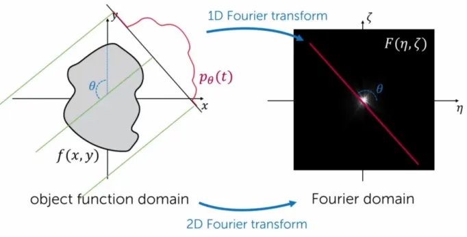
Figure 3-6: Schematic illustration of the Fourier slice theorem. The radon transform 𝑝𝜃𝑡 of a function 𝑓𝑥, 𝑦 is equaled to the line profile of the Fourier

transform of the same function at the angle 𝜃.[60] ... 38 Figure 3-7: Schematic illustration of (a) Pseodopolar fast Fourier transform,

(b) iterative reconstruction with constraints based on the Fourier slice

theorem.[64] ... 40 Figure 3-8: A collection of filters used in FBP. [65] ... 43 Figure 3-9: Principle of the ART method.[73] ... 47

Figure 3-10: (a) Reference image. Reconstruction images using simultaneous iterative reconstruction technique with 20 iterations (b) at 8 deg angular coverage, (c) at 15 deg angular coverage, (d) at 30 deg angular

coverage, (e) at 60 deg angular coverage, (f) at 120 deg angular coverage. ... 57

Figure 3-11: Patient with pulmonary nodules imaged by (A) chest

radiography, (B)-(C) digital chest tomosynthesis, (D) CT.[41]... 58

Figure 4-1: (a) Schematic diagram of the s-DBT system. The dots on the linear source array indicates multiple equal-spaced x-ray sources. (b) A

picture of the stationary digital breast tomosynthesis system. ... 62

Figure 4-2: (a) Schematics of the AFVR. The linear source array and each detector row cut the image space into a series of thin slabs. (b) A side view of image space, three fan volumes corresponding to three detector rows are

marked in the diagram. ... 63 Figure 4-3: A flow chart of the AFVR... 66

Figure 4-5: Schematic diagram of (a) 2D distance-driven method, and (b)

3D distance-driven method.[93] ... 69

Figure 4-6: FBP reconstruction of a head section: reference image,

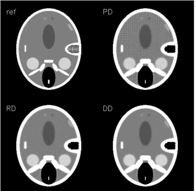
pixel-driven FBP, normalized ray-pixel-driven FBP, and distance-pixel-driven FBP.[115] ... 70

Figure 4-7: Iterative reconstruction of a head section using maximum likelihood (ML) algorithm: reference image, pixel-driven ML reconstruction, ray-driven ML reconstruction, and distance-driven ML

reconstruction.[115] ... 71

Figure 4-8: Enlarged view of (a) a Shepp-Logan phantom, AFVR-SIRT reconstruction of the Shepp-Logan phantom (b) using ray-driven projection

model, and (c) using the distance-driven projection model. ... 73

Figure 4-9: Reconstruction slice using (Left) ray-driven projection model,

and (Right) distance-driven projection model. ... 74

Figure 4-10: Line profile of the reconstruction slice using the ray-driven

projector and the distance-driven projector ... 75 Figure 4-11: Normalized MTF curves ... 77

Figure 4-12: Image of a fatty breast reconstructed by AFVR-SIRT and RTT.

... 79 Figure 4-13: Reconstructed breast image with carcinoma. ... 80 Figure 4-14: s-DCT system. ... 81

Figure 4-15: Reconstruction slices of an anthropomorphic chest phantom using two reconstruction methods. Left: AFVR reconstruction. Right: RTT

reconstruction. ... 83

Figure 4-16: Reconstruction slices of an anthropomorphic chest phantom using two reconstruction methods. Left: AFVR reconstruction. Right: RTT

reconstruction. ... 83

Figure 4-17: Reconstruction slices at 4 different positions of a chest

phantom reconstructed by AFVR. ... 84

Figure 4-18: A reconstruction slice of a patient imaged by s-DCT (a) before

Figure 4-21: Tooth phantom imaged by four imaging modalities: standard

2D digital bitewing, standard PSP bitewing, s-IOT, and micro-CT. [118] ... 89 Figure 4-22: Skin line artifacts in the breast tomosynthesis image. ... 94 Figure 4-23: Schematic of the skin line artifact reduction method.[119] ... 95

Figure 4-24: Reconstruction of one 2D fan volume (Top) without the skin

line artifact reduction, (Bottom) with the skin line artifact reduction. ... 96 Figure 4-25: Breast reconstruction slices after the correction. ... 97

Figure 4-26: A schematic of the truncation artifact reduction method. [119]

... 98

Figure 4-27: Cross-sectional reconstruction images of a patient’s breast (Top) without any correction, (Bottom) with the data truncation correction.

... 100

Figure 4-28: Reconstruction slices of a patient’s breast (a) without any

correction, (b) with the data truncation correction. ... 101

Figure 4-29: Reconstruction slices of a patient’s breast (a) without any

correction, (b) with the data truncation correction. ... 102

Figure 4-30: Breast segmentation using (a) Otsu’s threshold method (b)

iterative Otsu’s method. ... 105

Figure 4-31: 2D projection images with and without the density correction.

... 107

Figure 4-32: (a) Digital mammography image, (b) Synthetic mammography

with density correction and contrast enhancement ... 109 Figure 5-1: Flow chart of the f-SPR scatter estimation method. ... 119

Figure 5-2: (a) Stationary digital breast tomosynthesis (s-DBT) system with PSD installed. (b) The primary sampling device (PSD) designed for the s-DBT system is placed on the compression paddle. (c) Breast biopsy

phantom. (d) BR3D breast imaging phantom. ... 122

smooth and does not contain any noise. The ISPR estimated scatter though over/under estimates the scatter in the region with object features. The f-SPR estimation captures both the large scale smooth variation and the local

fluctuation of the scatter profile. ... 126

Figure 5-4: (a) Central projection view of the breast biopsy phantom. The index marks seven regions that are used in CR and SDNR analysis. (b) Enlarged views of region 1 and region 2 (from left-to-right: without scatter correction, SI corrected, ISPR corrected, and f-SPR corrected images). (c) The contrast ratio and SDNR for the seven ROIs. Both SI and f-SPR corrected images show a significant improvement in contrast ratio, but only f-SPR shows significant enhancement in SNDR. On average, a 58% increase in CR and 51% increase in SDNR are observed with f-SPR scatter

correction method. ... 127

Figure 5-5: In-focus reconstruction slice of the BR3D feature slab: (a) without scatter correction, (b) with ISPR, (c) with SI, and (d) with f-SPR scatter correction. All images are displayed at the same window width. The window level is set to be the average of the image intensity. Reconstruction with f-SPR correction has a significantly better SDNR compared to reconstruction with other scatter correction methods, and a CR comparable

to that in the reconstruction with SI correction. ... 128

Figure 5-6: Top left: in-focus reconstruction slice of two spheroid masses in the BR3D phantom (a) without scatter correction, (b) with ISPR, (c) with SI and (d) with f-SPR scatter correction. Top right: in-focus reconstruction slice of micro-calcifications in the BR3D phantom (a) without scatter correction, (b) with ISPR, (c) with SI and (d) with f-SPR scatter correction. All images are displayed at the same window width. Bottom: CR and SDNR

of three spheroid masses. ... 129

Figure 5-7: Human cadaver imaged by s-DCT. Projection image of the central view (a) without scatter correction, (b) with f-SPR scatter correction. Reconstruction image (c) without scatter correction, (d) with scatter correction. Images before and after f-SPR scatter correction are displayed at the same window width, but different window level, which is set to be

the mean gray value of the image. ... 131

Figure 5-8: Correlation of the scatter profile between the f-SPR estimation and the SI/ISPR estimation. The white line on the scatter map indicates the

area that is used to compute the correlation. ... 133

scatter-corrected reconstruction are the same as those of the f-SPR with no

filtering. The x axis is the standard deviation of the Gaussian filter. ... 134

Figure 5-10: Left: enlarged view of micro-calcifications in the in-focus reconstruction slice of the BR3D phantom: (a) without scatter correction, (b) with f-SPR scatter correction and (c) with direct Gaussian filtering on the SI corrected projection data (f-SI). Right: system MTF curve using different processing methods. It is clear that the f-SPR method has a negligible impact on the spatial resolution, while direct filtration of the SI corrected image with the same filter size dramatically reduces the spatial

resolution... 135

Figure 6-1: (a) Anatomy of a heart and the coronary artery. (b) A cross-section image of the coronary artery with plaque buildup and a blood clot,

which blocks the blood flow inside the heart... 140 Figure 6-2: An image of the coronary calcification imaged by CTA.[162] ... 141

Figure 6-3: (a) CT images, and (b) CT numbers of mimic coronary

calcifications with different calcium concentrations. ... 142

Figure 6-4: (a) Stationary digital chest tomosynthesis system developed by our team. (b) Explant heart model with injected calcium simulants. (c) The porcine heart inside an anthropomorphic chest phantom with inflated porcine lung. Unfortunately, the lung was damaged by the butcher and did

not stay inflated during the scan. ... 143

Figure 6-5: Mimic CAC in explant heart model imaged by both s-DCT and

CT. Red and yellow circles mark the locations of the CAC. ... 146 Figure 6-6: Calcium score derived from CT and tomosynthesis images. ... 147

Figure 6-7: Reconstruction slices of heart samples with the anthropomorphic chest phantom. Mimic CACs are shown in (a), (c)

tomosynthesis reconstruction slices, and (b), (d) CT reconstruction slices. ... 148

Figure 6-8: Calcium scores of the heart samples inside chest phantom

LIST OF ABBREVIATIONS

2D Two Dimensional

3D Three Dimensional

AVFR Adapted Fan Volume Reconstruction BLOBS Kaiser-Bessel Basis Functions

BP Back Projection

CAC Coronary Artery Calcification CACS Coronary Artery Calcium Scores

CC Cranial Caudal

CG Conjugate Gradient

CNT Carbon Nanotube

CR Contrast Ratio

CPU Central Processing Unit

CT Computed Tomography

CTA Computed Tomography Angiography

CXR Chest X-ray Radiography

DBT Digital Breast Tomosynthesis DCT Digital Chest Tomosynthesis

DD Distance-driven

DE Dual Energy

DICOM Digital Imaging and Communications in Medicine

EM Expectation Maximization FBP Filtered Back Projection FDA Food and Drug Administration GPU Graphics Processing Units

f-SPR Filtered Scatter-to-primary Ratio

ICD Iterative Coordinate Descent

ISPR Interpolated Scatter-to-primary Ratio LAD Left Anterior Descending Artery

LCX Left Circumflex Artery

LM Left Main Artery

MLO Mediolateral oblique

MTF Modulation Transfer Function

OS Ordered Subs et

PCG Preconditioned Conjugate Gradient

PD Pixel-driven

PDA Posterior Descending Artery

PSD Primary Sampling Device

RCA Right Coronary Artery

RD Ray-driven

ROI Region of Interest

RTT Real Time Tomography

SDNR Signal difference to noise ratio SI Direct Scatter Interpolation

s-IOT Stationary Intraoral Tomosynthesis SIR Statistical Iterative Reconstruction

SIRT Simultaneous Iterative Reconstruction Technique SNR Signal to noise ratio

SPR Scatter to primary ratio

TV Total Variation

UNC University of North Carolina

CHAPTER 1: Introduction

1.1 Dissertation Overview

Lung cancer and breast cancer are the two leading causes of cancer death in the United

States. Based on a recent study by American Cancer Society, an estimated of 220,000 new cases of lung cancer and 250,000 new cases of breast cancer are diagnosed in 2016, and about 200,000

deaths from breast and lung cancers.[1] For both cancers, early detection is extremely important as it can dramatically reduce the mortality rate.

Currently, two dimensional (2D) x-ray imaging modalities, such as chest radiography and

digital mammography, are widely used for non-invasive cancer and disease screening. The 2D x-ray imaging techniques have the advantages of low cost and low radiation dose, therefore they are

well suitable for large population disease screening. However, in 2D images, the depth information of the three dimensional (3D) object is missing; structures at different depths overlap on each other,

severely degrading the image contrast and cause image artifacts. As a result, the 2D imaging techniques suffer from low diagnostic sensitivity and specificity.

Computed Tomography (CT) was invented to address the drawbacks of 2D x-ray imaging.

In CT, hundreds of 2D x-ray measurements are acquired at various imaging angles and are used to compute the 3D image of the object. This completely removes the structure overlapping artifact

Digital tomosynthesis (DTS) is another tomographic technique which produces pseudo-3D images at a radiographic dose level. Unlike CT which acquires hundreds of x-ray images, DTS

only take a few x-ray projections to compute the 3D image, this results in a much lower radiation dose and a lower-cost system compared to CT. It has been shown that DTS has an improved

diagnostic accuracy over the 2D radiography in many clinical applications, including abdominal, breast, chest, dental, musculoskeletal and sinonasal imaging.[2]–[7] Most DTS systems use a single x-ray source and a mechanical moving gantry to shoot X-ray at different imaging positions.

This mechanical translating design leads to image blur and slows down the scanning speed which potentially causes more patient motion blur.

Stationary digital tomosynthesis (s-DTS) system eliminates the source motion in the conventional DTS system with a source array consisted of multiple fixed carbon nanotube (CNT) based x-ray sources.[2], [8]–[10] Each CNT source in s-DTS is switched electronically, thus the

s-DTS is capable of performing cardiac gated imaging which can significantly reduce the patient motion blur in the cardiac imaging and the pediatric imaging.[11] Previous studies have shown

that the s-DTS has improved image resolution as well as faster scanning time compared to the conventional DTS.[8], [10], [12]

Image reconstruction is the process to reconstruct 3D images of the scanned object from

2D x-ray measurement. It is a crucial component in tomosynthesis imaging as the reconstruction algorithm would directly affect the final image quality. Compared to regular CT, DTS suffers from

shown that SIR produces better reconstruction images over the classical filtered back projection (FBP) algorithm.[13], [20]–[22] However, SIR is computationally expensive. The reconstruction

could take several hours, and it is not practical in a clinical setting.

In this dissertation, a fast iterative image reconstruction algorithm, named adapted fan

volume reconstruction, for linear tomosynthesis systems will be proposed. The image artifact reduction methods and the synthetic mammography technique will be discussed. Next, a measurement-based scatter correction algorithm will be introduced. The feasibility of assessing

heart calcium score using stationary digital chest tomosynthesis (s-DCT) will be investigated.

1.2 Research Objective

1.2.1 Iterative Reconstruction for s-DTS

In this aim, a fast iterative reconstruction algorithm, named adapted fan volume

reconstruction (AFVR), was developed to reconstruct s-DTS images with linear source array. A comparison study was performed to investigate the reconstruction image quality of the proposed AFVR and the classical FBP algorithm. In addition, two different forward projectors were

investigated and image processing techniques for image artifacts reduction were implemented. Furthermore, the AFVR was implemented on three s-DTS system: the s-DBT, the s-DCT, and the

stationary intraoral dental tomosynthesis (s-IOT) system. Finally, the method for generating synthetic mammography was investigated.

1.2.2 Scatter Correction

scatter correction algorithm development for scatter estimation and compensation. The scatter correction method was evaluated on the s-DBT system using breast phantom, and it was also

implemented on the s-DCT system to remove scatter in human cadaver images.

1.2.3 Quantitative Tomosynthesis Imaging

In this phase, the feasibility of assessing heart calcium score using the s-DCT system was studied. A heart model was developed, and imaged by both CT and s-DCT ex vivo. The calcium

score metric for chest tomosynthesis was then developed, and the correlation between CT-derived calcium score and the tomosynthesis-derived calcium score was studied.

1.3 Outlines of Dissertation

This dissertation is organized in the following order: (1) background of tomosynthesis

imaging, (2) iterative reconstruction for tomosynthesis, (3) measurement-based scatter correction algorithm, (4) quantitative tomosynthesis imaging. Chapter 2 introduces the underlying principles of x-ray imaging, the DTS and s-DTS. Chapter 3 provides the mathematical foundation of image

reconstruction. In Chapter 4, a fast iterative reconstruction algorithm for s-DTS is reported. Chapter 5 investigates the scatter correction methods for s-DTS and reports the filtered

scatter-to-primary ratio (f-SPR) scatter estimation. Chapter 6 studies the feasibility of assessing calcium score using s-DCT. Finally, in Chapter 7, the dissertation is summarized and the future direction

of the research is discussed.

 C. R. Inscoe, G. Wu, at el (2017)

Stationary intraoral tomosynthesis for dental imaging.

 C. Puett, J. Calliste, G. Wu, at el (2017)

Contrast enhanced imaging with a stationary digital breast tomosynthesis system.

 J. Calliste, G. Wu, at el (2016)

A new generation of stationary digital breast tomosynthesis system with wider angular

span and faster scanning time.

 J. L. Goralski, A. Hartman, G. Wu, at el (2016)

Digital chest tomosynthesis as a novel method for 3d lung imaging.

 Y. Z. Lee, J. L. Goralski, A. Hartman, G. Wu, at el (2016)

Stationary digital chest tomosynthesis of cystic fibrosis.

 A. E. Hartman, J. Shan, G. Wu, at el (2016)

Initial clinical evaluation of stationary digital chest tomosynthesis.  G. Wu, at el (2016)

Stationary digital chest tomosynthesis for coronary artery calcium scoring.

 C. R. Inscoe, G. Wu, at el (2015)

Low dose scatter correction for digital chest tomosynthesis.

 J. Shan, A. Tucker, L. R. Gaalaas, G. Wu, at el (2015)

Stationary intraoral digital tomosynthesis using a carbon nanotube X-ray source

array.

 J. Shan, L. Burk, G. Wu, at el (2015)

Adapted fan-beam volume reconstruction for stationary digital breast tomosynthesis.

Parts of the work presented in the thesis has resulted in the following patent applications:  Digital tomosynthesis systems, methods, and computer readable media for intraoral

dental tomosynthesis imaging”

U.S. Patent: 15/205,787. Filing on Jul 8, 2016.

 Intraoral tomosynthesis systems, methods, and computer readable media for dental

imaging

CHAPTER 2: X-ray Imaging

2.1 X-ray Interactions with Matters

X-ray is discovered by German physicist Wilhelm Röntgen, who studied the Crooks tubes

and noticed a green glow on a nearby fluorescent screen even though the tube was wrapped by black cardboards. Röntgen realized that it must be due to some invisible rays generated from the

Crooks tube, and he referred the rays as “X-rays” to indicate the unknown type of this radiation. Röntgen also took a picture of his wife’s hand on a photographic plate using x-ray (Figure 2-1), which became the first medical use of x-ray. [23]

light. The difference between x-ray and visible light is that x-ray has a much smaller wavelength that ranges from 0.1 pm to 10 nm, corresponding to an energy level from 100 eV to 10 MeV. The

smaller wavelength and higher energy of x-rays give it the ability to penetrate through most materials. This ability, however, does not come without any cost. The x-ray interacts with the

matters while it penetrates through, and these interactions weaken the x-ray intensity until finally, it reaches zero. In medical imaging, the three major types of interactions between x-ray and matters are (1) Photoelectric absorption, (2) Compton scattering, and (3) Rayleigh scattering. These

interactions are illustrated in Figure 2-2.[25] Here, we briefly introduce the three major x-ray interactions as they directly contribute to the contrast in x-ray imaging.

2.1.1 Photoelectric Absorption

In Photoelectric absorption, an electron of the atom is freed by the incident x-ray photon,

and be emitted from the atom. (Figure 2-2B) The difference between the incident photon energy and the binding energy of the electron becomes the kinetic energy of the emitted electron, which is also called photoelectron. When the emitted electron is at a low state, electrons at high energy

state will jump to this lower state, resulting the characteristic x-ray with energy equals to the energy difference between the two states.

Approximately, the occurrence rate of photoelectric absorption is proportional to 𝑍3⁄𝐸3, where Z is the atomic number of the material and E is the energy of the incident x-ray photon.[26]

harmful to the human body, as it ironizes the atoms and could potentially breaks the molecular bonds of DNA and proteins.

Figure 2-2: Interactions of x-ray. (A) X-ray beam does not interact with the material, (B) Photoelectric absorption and characteristic x-ray, (C) Rayleigh scattering, (D) Compton scattering where recoiled electron is generated. [25]

2.1.2 Compton Scattering

Compton scattering is the predominant interaction in the diagnostic energy range with soft

tissue, it is illustrated in Figure 2-2. In Compton scattering, the incident photon transfers a portion of its energy to the electron, which causes a recoil and removal of the electron, the incident photon will change direction after the interaction. However, the total energy and momentum are conserved

(> 100 keV), the probability is approximately proportional to 𝑍 𝐸⁄ .[25] As shown in Figure 2-3, Compton scattering consists the majority of scatter radiation, which is an important issue for diagnostic imaging as it reduces the image contrast and causes artifacts.

2.1.3 Rayleigh Scattering

In Rayleigh scattering, the incident photon temporarily excites an electron without freeing it from the atom. When the electron returns to its original state, it emits an x-ray photon with the

same energy but a different direction of the incident photon. This process is also known as coherent or elastic scattering, where the photon energy does not change. Rayleigh scattering does not transfer the energy of x-ray photon to the material, therefore, it does not contribute to patient

radiation dose. However, Rayleigh scattering is an important issue for x-ray imaging as it can be up to 20% of the scattering. The probability of the Rayleigh scattering is approximately

proportional to 𝑍2⁄𝐸2, therefore, it is more likely to occur with low energy x-ray photons and high

Z materials.[25]

2.2 X-ray Attenuation and the Beer–Lambert law

The interactions of x-ray with matters have a combined effect of attenuating the x-ray intensity, this relationship is experimentally determined and it can be approximated as:

∆𝐼 𝐼⁄ = −𝜇∆𝑥, (2-1)

time, it is considered to only depends on the material composition. Figure 2-3 illustrates the relationship between the mass attenuation and the x-ray photon energy, and the contributions on

the attenuation from different x-ray interactions.[27] For the x-ray used in medical imaging (30 keV – 120 keV), the major mass attenuation comes from the Compton scatter.

Figure 2-3: Mass attenuation of tissues at different photon energy.[27]

The relationship described by Equation 2-1 is often written in an integral format:

𝑰 = 𝑰𝟎𝒆− ∑ 𝝁𝒊 𝒊𝒙𝒊, (2-2)

where 𝐼 is the x-ray intensity after it leaves the medium, 𝐼0 is the ray intensity before the x-ray enters the medium and interacts with the matters, 𝜇_𝑖is the mass attenuation within the mediumi,

and 𝑥𝑖 is the distance the ray travels within medium i. This exponential decay relationship is also referred as Beer–Lambert law, and will be used to model the image reconstruction problem. The

linear attenuation coefficient 𝜇 is a function of the interacted material and the x-ray energy spectrum, this forms the physics foundation of many x-ray imaging modalities.

2.3 X-ray Imaging Modalities

An ray image measures the interactions of ray and matters. The most widely used

x-ray image is the attenuation image, where the x-x-ray photons that leave the materials after being attenuated are recorded. As the x-ray attenuation depends on the atomic number of the material,

the attenuation value can differentiate/visualize materials with different densities. Besides attenuation, other physical effects, such as characteristic x-ray emission and scatter interactions, are also utilized to develop imaging techniques, such as x-ray spectroscopy, x-ray crystallography

and x-ray scatter imaging. In this study, we will only focus on the x-ray attenuation imaging techniques used in medical applications.

2.3.1 Radiography

Radiography is probably the oldest x-ray imaging technique, which is discovered along

with x-ray. In x-ray radiography, the patient is illuminated by a short x-ray pulse, and the x-ray photons exit patient are recorded in a 2D image. Due to the simplicity of the imaging system and the low cost, radiography is widely used in many medical applications, such as screening lung and

heart diseases in chest imaging, diagnosing abdominal diseases, detecting gallstones or kidney stones, detecting bone fractures as well as tooth cavities. Radiography image is originally recorded

on photographic films.

Based on the image receptor, radiography can be classified into three types: conventional

those benefits, the digital detector also has a high radiation dose efficiency and it lowers the radiation dose delivered to the patients.[28] The image post-processing and computer aided

diagnosis also become much easier on digital images.

One of the most common uses of x-ray radiography is in chest imaging for patients with

known or suspected lung diseases. The chest x-ray radiography (CXR) often acquire multiple views images with each view obtained at different orientations of the chest and the x-ray beam directions. Common CXR views include posteroanterior view, anteroposterior view, and lateral

view. As CXR only produces 2D images, multi-view radiographic images can help to visualize features at various positions inside the patient’s body. A schematic diagram of the CXR is shown

in Figure 2-4. [28]

Based on the characteristics of x-ray attenuation, the higher energy of the x-ray, the fewer interactions the x-ray would have with materials. Thus, high energy x-ray photons are much easier

to penetrate through the human body, however, they would have a lower sensitivity on differentiating different organs due to fewer interactions. CXR typical uses an x-ray source

operated at 120 kVp, which is optimized to balance body penetration as well as tissue contrast.

Although digital radiography works well on high contrast organs, it has poor contrast on soft tissues. The main reason lies in the imaging mechanism, in which radiography projects the 3D

object onto a 2D detector and the depth information of that object is lost in the radiographic image. As a result, features, such as different organs, overlap each other on the radiographic images, which

blurs the images and reduces the contrast, making it harder to identify diseases and extract useful diagnostic information.

2.3.2 Mammography

Mammography is another 2D radiographic imaging technique. Unlike radiography which is used in various different applications, mammography is only used for breast imaging and it has

a unique system design optimized for this specific goal. Originally, like radiography, mammography is recorded on the photographic film. Currently, the conventional film is replaced

by the digital detector. Equipped with a digital detector, the name of the imaging technology changes digital mammography (DM). A mammography exam, often called a mammogram, aids in the early detection and diagnosis of breast diseases in women. It has been shown that

mammogram is effective in screening breast cancer and reducing the mortality rate of the breast cancer.[29], [30] In fact, the American College of Radiology recommend screening mammography

every year for women, beginning at age 40.

As breast consists mostly of the soft tissue, the x-ray source used in digital mammography

customized x-rays for different patients. For example, for patients with thick breast, a longer pulse of higher energy x-rays would be generated to image breast. In DM, there is compression paddle

that compresses and fixes the breast on the detector during the scan. The compression paddle not only reduce the motion artifact, but it also measures the thickness of the breast which is used by

AEC to determine the source energy and exposure time for the specific patient. An illustration of the mammogram is shown in Figure 2-5.[31]

Figure 2-5: Illustration of the mammogram.[31]

DM uses a high-resolution detector with a pixel size around or smaller than 100 µm, to

right above the patient. CC view clearly depicts the entire breast including the nipple, the fat and the fibro-glandular tissue. MLO view images breast from the center of chest outward to the side,

it gives the best lateral view of the breast where pathological changes are most likely to occur. Examples of CC view and MLO view mammography images are shown in Figure 2-6.[32]

Figure 2-6: Digital mammography in (a) CC view and (b) MLO view.[32]

2.3.3 Computed Tomography

Computed tomography (CT) was invented in the 1970s by Godfrey Hounsfield and Allan Cormack. The basic idea of CT is using multiple 2D radiography images acquired at different

parallel beam design, it is soon being replaced by fan beam x-ray radiation for faster scanning speed. The initial axial imaging scheme is replaced by a helical or spiral scan for the purpose of

scan the entire organs in a single breath hold. Later, the cone beam CT is developed to achieve isotropic spatial resolution and an even faster scanning speed. Despite different system designs, a

typical CT system has one x-ray source tube mounted on a mechanical moving gantry and a digital detector that measures the x-ray radiation. The x-ray source rotates and fires x-rays at different spatial positions, the detector moves together with the source and measures the x-ray radiation for

each shoot. Each x-ray shoot forms a projection image in the CT exam, the x-ray source typically moves between 180 to 360 deg around the object and it generates hundreds of projection images

during one scan. The projection images are then transferred to a computer, and a specific computer software computes the 3D attenuation images of the object based on the projection images as well as the imaging geometry for each projection. This process is also called image reconstruction,

which will be intensively discussed in Chapter 3 and Chapter 4. A schematic diagram for a fan-beam axial CT is shown in Figure 2-7.[33]

In CT images, the image brightness, or image intensity, represents the linear attenuation, and the difference in the x-ray attenuation creates the contrast between different materials. The linear attenuation has a physical unit of cm-1_{. It is normally not necessary to record the exact value}

of the attenuation which would cost extra storage space, and it is also not convenient to interpret diagnostic information using a float number. Thus, in CT, the linear attenuation is truncated and

converted to an integer with a special unit called Hounsfield unit (HU), or CT number. The conversion from cm-1 to HU is:

𝜇(𝑖𝑛 𝐻𝑈) = 1000 ∙ 𝜇 − 𝜇𝑤𝑎𝑡𝑒𝑟 𝜇_{𝑤𝑎𝑡𝑒𝑟}− 𝜇_𝑎𝑖𝑟,

where 𝜇_{𝑤𝑎𝑡𝑒𝑟} and 𝜇_𝑎𝑖𝑟 are the linear attenuation of water and air, respectively. The CT images are typically

stored as a 16 bit image in the Digital Imaging and Communications in Medicine (DICOM) format. The

HU is converted to non-negative integer for storage and transfer, the conversion parameters are stored in

the image header, or DICOM header.

Figure 2-7: Third generation axial fan-beam CT geometry.[33]

CT produces 3D images of the patient anatomy with no tissue overlapping artifact, this

dramatically improves the image contrast and consequently the diagnostic accuracy over the conventional radiography. However, due to the large numbers of projection images acquired, CT delivers a significant amount of radiation dose to the patient, which is about 100 times the

studies on advanced image reconstruction algorithms showed promising results in reducing the radiation dose of CT, however, the diagnostic accuracy of those techniques are still the subject of

debate and more investigations need to be performed before the dose can be reduced clinically.[18], [34]–[36] In summary, although CT has many successful medical applications, it

is not a good choice for disease screening in the general public, and low dose 3D imaging modalities are still needed.

2.3.4 Digital Tomosynthesis

Digital tomosynthesis (DTS) is another tomographic imaging technique. Similar to CT, DTS also produces 3D images from multiple projections acquired during one scan. However, DTS

only acquires a few projection images, which is only a fraction of the projection images in CT, within a much smaller angular coverage. This imaging mechanism simplifies the system design,

as a result, DTS has lower cost over CT and it delivers a radiographic dose level radiation dose to the patient. A schematic diagram of tomosynthesis is illustrated in Figure 2-8(a), where three projection images are acquired at different source position. Figure 2-8(b) demonstrate the principle

of the 3D tomosynthesis. In single x-ray projection image, features in various depths of the imaged object overlap each other. By shift-and-add multiple projection images with different imaging

geometries, in-focus planes with different features will be obtained and the overlapping artifact is substantially reduced.

other normal tissues in the 2D mammography, its contrast further reduces. As a result, the call back rate is quite high for digital mammography as doctors cannot tell whether the suspected lesion

truly exist. DBT has been demonstrated to significantly improve the contrast of the lesion by reducing the overlapping artifact with the 3D images.[3], [32], [37], [38] For microcalcifications,

however, the digital mammography performs better than DBT as the source motion in DBT blurs the small calcifications.[4], [39] As a result, DBT is FDA-approved to be used together with DM for breast cancer screening, where DBT is used for confirming lesions and DM is used for

visualizing micro-calcifications. Some DBT systems, such as the SenoClaire 3D Breast Tomosynthesis manufactured by GE Healthcare, use step-and-shoot imaging to reduce the source

motion artifact. However, this also increases the scanning time, which potentially introduces more patient motion, as well as the patient discomfort.

Figure 2-9: Illustration of DCT.[40]

Another important application for DTS is chest imaging, in which the DTS is called digital chest tomosynthesis (DCT). The basic principle of DCT is similar to DBT. As illustrated in Figure

2-9,[40] DCT consists an x-ray source mounted on the moving gantry, a digital detector and the control electronics. The gantry moves the source to various projections and multiple projection images are acquired. The difference between DCT and DBT are in the system design, where harder

x-rays, larger angular span, and more projection images are used in DCT. For chest imaging, the most challenging task is the detection of pulmonary nodules, which are strongly related to the lung

the diagnostic accuracy of lung nodules over CXR with a comparable sensitivity as CT for large lung nodules.[41]–[43]

The 3D tomosynthesis images reduce the overlapping artifact and lead to higher diagnostic accuracy over the 2D radiography in many applications. However, DTS has many challenges as

well. First, the limited angular coverage and the small projection images in DTS are mathematically not sufficient to restore the full 3D information of the imaged object. As a result, tomosynthesis images have a poor depth resolution, lower contrast and move artifacts over CT.

Secondly, the mechanical moving gantry slows down the scanning speed and introduces two types of motion artifact. First, the rotating source introduces motion blur to the projection image, which

in terms adversely affect the image resolution and the diagnostic accuracy for small features. For example, DBT suffers from the source motion blur and performs worse than 2D mammography in detecting microcalcifications. Another type of motion artifact is the indirect patient motion artifact

caused by long scanning time. In fact, the patient motion blur, including heart beats and respiration, is the most destructive image artifact for chest imaging.

2.4 Stationary Digital Tomosynthesis 2.2.1 Field Emission Effect

Field emission, also known as field electron emission, is the emission of electron induced by an external electric field. Field emission is first observed in eighteen centuries, but not until

𝐼 = 𝑎𝑉2exp (−𝑏𝜙 3

𝛽𝑉 ), (2-4)

where a, b are two constants, and I, V, 𝜙, 𝛽 are the emission current, voltage of the applied field, work function, and field enhancement factor, respectively.

An important application of field emission is making field electron emitters or electron gun

source. Traditionally, electrons are generated based on thermal electron emission, where electrons are emitted when the metallic emitter is heated up to a high temperature. However, the field

emission only requires external electric field and it has no requirement of the temperature. Hence, field emission is often called “cold emission” or “cold cathode emission”, and the electron

generated from field emission is often all “cold electrons”.

Figure 2-10: Illustration of the field emission. [45]

2.2.2 CNT Field Emitter

unprecedented interest in the CNT and opened a new era of nanotechnology.[46] Figure 2-11 illustrates the nanostructure of a single wall CNT.[47] Based on the number of layers, CNT can be

categorized as single-walled nanotubes (SWNTs) or multi-walled nanotubes (MWNTs). The diameter varies between SWNTs and MWNTs. The diameter for SWNTs ranges from 0.4 nm to

10 nm, while those of MWNTs are much larger, which ranges from 2 nm to over 100 nm. Depends on the nanostructure or the ways that CNT is created, CNT can have a variety of mechanical, optical and electrical properties, leading to wide applications including medical implant,

semiconductors, batteries and more.[47]

Figure 2-11: Illustration of the CNT nanostructure.[47]

CNT has been extensively studied as a field emitter. The main reason is that CNT has a high aspect ratio, which allows the electron tunneling the energy barrier more easily and makes the field emission to be naturally enhanced. CNT field emitter presents many advantages over

thermionic emission. First, CNT field emitters do not require heating to generate electron, which is more energy efficient and produces more stable electron focusing. The cold nature of field

emission also simplifies the cooling system design. Secondly, CNT field emitter could be electronically switched on and off, which is faster than the thermionic emitter and eliminates the need of a mechanical shutter. Finally, the CNT field emitter has more compact design over the

Figure 2-12: A schematic diagram of the triode-type field emission x-ray source. Electron emission controlled by the voltage applied to the SWNTs. Electrons accelerate inside the vacuum chamber and x-rays are generated when accelerated electrons hit the copper target.[48]

Our lab developed the first CNT-based x-ray source using a cold cathode made of SWNTs.[48] A systematic diagram of the first CNT-based radiography system is shown in Figure

2-12. The source target was made of copper, and the anode voltage was set to be 14 kV. The whole assembling was sealed inside a vacuum chamber. Over the past decade, our lab has developed several CNT-based x-ray source and source array with various source voltage, focal spot size, and

tube output for different applications, including micro-CT system,[49]–[51] microbeam radiotherapy system,[52], [53] stationary CT system,[54] stationary digital breast tomosynthesis

system,[9], [10], [55] stationary digital chest tomosynthesis system and the stationary intraoral tomosynthesis system.[2], [8] Figure 2-13(a) shows a micro-CT system using a CNT-based x-ray

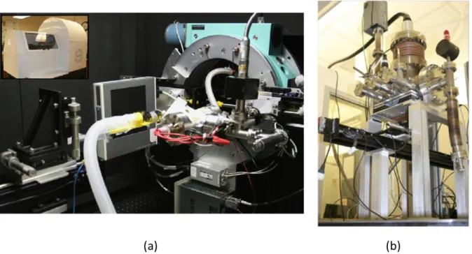
Figure 2-13: (a) A micro-CT system using a CNT-based x-ray source. (b) a desktop microbeam radiation therapy system with CNT-based x-ray sources.

2.2.3 Stationary Digital Tomosynthesis

As mentioned previously, the mechanical translating gantry used in DTS has several drawbacks, it slows down the scanning speed and introduces source motion blur. Based on the

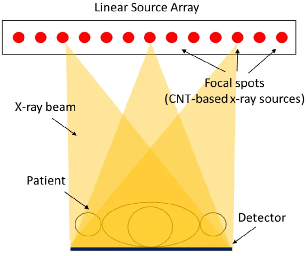
field emission technique, our lab developed a stationary digital tomosynthesis (s-DTS) technology, where the sources stay stationary during the scan. As shown in Figure 2-14, in s-DTS, the moving gantry and the “hot” x-ray source are replaced by a “cold” source module made with multiple

CNT-based x-ray sources. All CNT-based x-ray sources are fixed on the source ensemble, each CNT-based x-ray source or focal spot has its unique spatial position on the source ensemble and it

with the translating gantry. For instance, we have developed a source ensemble with crossing lines geometry where two linear arrays of sources crossed at the middle, and a square-shaped source

array where sources are distributed along the edge of the square.

Figure 2-15: (a) A picture of the stationary digital breast tomosynthesis system. The linear source array with CNT-based x-ray sources is retrofitted onto a Hologic Selenia Dimensions tomosynthesis system.

Based on the clinical applications, three s-DTS systems have been developed in our lab:

the stationary digital breast tomosynthesis, the stationary chest tomosynthesis, and the stationary intraoral tomosynthesis. Pictures of s-DBT and s-DCT are shown in Figure 2-15. Each

tomosynthesis system targets a unique clinical application. As a result, the x-ray sources used in each system are designed to have different tube voltage, tube current, and focal spot size. For

array much easier, and also, as we will discuss later, allows a unique way to reconstruct images which turns out to be significantly faster than the conventional reconstruction algorithms.

s-DTS has a couple advantages over conventional DTS: first, the source motion, as well as the induced image blur are eliminated in s-DTS, resulting in an improved image resolution at the

same detector and source focal spot; second, by eliminating the gantry motion in DTS, the total scanning time reduces in s-DCT. Consequently, the patient motion blur is also reduced; thirdly, each CNT-based x-ray source is electronically switched on and off, this enables precise control of

CHAPTER 3:Image Reconstruction

Image reconstruction is a crucial part for 3D imaging modalities, including CT and DTS, as it converts the 2D raw data to nice 3D images and directly affects the quality of the images used for disease diagnosis. In this chapter, we will briefly introduce the fundamentals of image reconstruction, the system modeling including basis function, forward and back projection. We will then walk through different reconstruction methods, from the analytical filtered back projection method to the algebraic iterative reconstruction method, and finally, the statistical iterative reconstruction method which works extremely well for low dose and under-sampling image reconstruction problems. Since most reconstruction algorithms are originally developed with the assumption of complete sampling, we will introduce the concept of each reconstruction method in the context of CT reconstruction.

3.1 System Modelling 3.1.1 Linearization

As Beer’s law suggests, the ray imaging is a non-linear process since the number of

x-ray photons decreases exponentially as the x-x-rays pass through materials. Solving this non-linear problem is typically much harder than solving a linear problem. Therefore, many reconstruction

algorithms, including the famous FBP algorithm, first convert the imaging process to a linear system and then solve the linear problem. Note that the Beer’s law (Equation 2-2) states an exponential decay of the x-ray beam intensity, thus, the linearization can be achieved by applying

a logarithmic transformation to both the blank data 𝑰0, a measurement of x-ray beam intensity

ln(𝑰) = ln(𝑰𝟎𝒆− ∑ 𝝁𝒊𝒙𝒊𝒊 )

ln 𝑰 = ln 𝑰₀∙ (− ∑ 𝝁_𝒊𝒙_𝒊 𝒊

)

ln (𝑰0

𝑰) = ∑ 𝝁𝒊 𝒊𝒙𝒊 .

(3-1)

The result of the linearization is often called a line integral image, where the photon counts in the

raw data are converted to a summation of the linear attenuation coefficients for each source detector pair.

It should be noted that some reconstruction algorithms, e.g. the Maximum Likelihood Expectation Maximization algorithm, do not require the linearization step and uses photon counts during the reconstruction.[56], [57] Although these methods model the system more accurately,

they generally run slower than those algorithms require linearization. In this thesis, I will focus on the group of reconstruction methods that requires linearization, and the measurement or the

measured data mentioned shown later in the thesis refers to the projection data after the logarithmic transformation.

3.1.2 Basis Function

Inside the computer, all data is stored and processed in discretized digits. A continuous

attenuation image 𝜇(𝒓), therefore, is discretized in both space and intensity. While the intensity of the linear attenuation is discretized into a fixed precision (i.e. single precision or double precision),

the space is discretized using a set of basis functions {𝑏_𝑖(𝒓) ∶ 𝑖 = 1, … , 𝑛_𝑣}:

𝜇(𝑟) ≈ ∑ 𝜇𝑖𝑏𝑖(𝑟) 𝑛𝑣

𝑖=1

where 𝑛𝑣 is the number of basis functions. The more basis functions used, the more accurate will

be the discretization. Substituting the above expression for 𝜇(𝒓) to Equation 3-3, we will have:

∫ 𝜇(𝑟)𝑑𝑟 𝑙

≈ ∫ ∑ 𝜇𝑖𝑏𝑖(𝑟)𝑑𝑟 𝑛𝑣

𝑖=1 𝑙

= ∑ 𝜇𝑖∫ 𝑏𝑖(𝑟)𝑑𝑟 𝑙

𝑛𝑣

𝑖=1

= ∑ 𝐴_𝑖𝑗𝜇_𝑖 𝑛𝑣

𝑖=1

≡ 𝐀𝝁,

(3-3)

and

A_𝑖𝑗 = ∫ b_𝑖(r)dr l

. (3-4)

The matrix𝐀 in Equation 3-3 is called the system matrix or the system model, as it describes the imaging process. Applying the system matrix 𝐀 on the image 𝝁 is called a forward projection, as it projects 𝜇(𝒓) to the measured data. On the other hand, applying the transpose of the system matrix 𝐀𝑇 on a data vector is called a back projection and it is often used to update the current

estimation of 𝜇. Forward projection and back projection are two key elements in the image reconstruction, they consume the most of the computation time in iterative reconstruction methods.

Basis function determines the accuracy of the discrete representation of the continuous object. In addition, basis function affects the implementation of the system model and the

convergence rate of the iterative reconstruction algorithms. It is preferred to use basis function that is computationally efficient without scarifying the representation accuracy. Pixel (or voxel for 3D images) is a widely used basis which represents a continuous image with a rectangle function as

shown in Figure 3-1(a):

𝑏(𝑟) = {1, |𝑟 − 𝑟0| < 𝑝/2

where p is the pixel size. Pixel basis is simple and computationally inexpensive. With pixel basis, several computationally efficient projection models have been developed, including pixel-driven

model, ray-driven model, distance driven model, separate footprint model, and Fourier space model. Pixel basis is not smooth, as shown in Figure 3-1(b). Furthermore, as the Fourier transform

of a rectangle function has a large side-lobe amplitude, pixel basis could amplify errors.

Figure 3-1: (a) Line profile of the rectangle function used in pixel basis with the pixel size of 1. (b) a smooth signal that is represented with pixel basis. [58]

Smooth basis functions, such as blobs and B-splines, have been proposed as attractive alternatives. Introduced by Lewitt,[59] the Kaiser-Bessel basis functions (blobs) are spherically symmetric function as shown in Figure 3-2(a):

𝑏(𝑟) = {

𝐼_𝑚(𝛼√1 − (𝑟 𝑎⁄ )2₎

𝐼_𝑚(𝛼) (√1 − (𝑟 𝑎⁄ )2) 𝑚

, 0 < 𝑟 < 𝑎 0, 𝑜𝑡ℎ𝑒𝑟𝑤𝑖𝑠𝑒

. (3-6)

where 𝐼_𝑚 is a modified Kaiser-Bessel function of order m, r is the radial distance. 𝛼 is a parameter that controls the shape of the blob, a smaller 𝛼 will result a fatter shape of the blob. a is the radius of the blob. A blob with larger radius would lead to more overlaps with neighboring blobs and

consequently more expensive computation.

3.1.3 Pixel-driven Method

The pixel-driven (PD) model is the first proposed projection method for CT

reconstruction.[60] As shown in Figure 3-3, in PD projection model, both the image voxel and the

detector pixel are modeled as points. Each image voxel, shown as 𝑃12 in Figure 3-3, is projected onto the detector, which is indicated as a red dot in Figure 3-3. The contribution of the attenuation

from this pixel to the detector pixels, 𝐷₂₃ and 𝐷₃₄, is inverse proportional to the distance between the intersection point and the detector pixels. A linear (1D case) or bi-linear (2D case) interpolation is typically used to compute the weighting. Similarly, for back projection, a detector pixel is back

projected, based on the imaging angle, onto the image space. Based on the distance between the intersection point and its surrounding voxels, an interpolation is perform and the weightings are calculated. PD forward and back projector will introduce high-frequency artifact to the

PD model, such as reducing the size of the voxel, have been investigated, which were shown to reduce the aliasing artifact but with a more expensive computation.

Figure 3-3: Pixel-driven forward and back projector. [58]

3.2 Analytical Image Reconstruction 3.2.1 Radon Transform

The x-ray project a high dimensional object to a lower dimensional detector measurement, this process is mathematically described by the Radon transform, which was introduced in 1917

by Johan Radon. More strictly, the Radon transform is the integral transform which takes a high

the detector function 𝑝𝜃(𝑡) is obtained. We say the detector function 𝑝𝜃(𝑡) is the Radon transform

of the function 𝑓(𝑥, 𝑦):

ℛ𝑓(𝜃, 𝑡) = ∫ 𝑓(𝑥, 𝑦)𝑑𝑠 𝐿(𝜃,𝑡)

= 𝑝_𝜃(𝑡). (3-7)

The 𝑥-𝑦 and the 𝜃-𝑡 follows the relationship:

𝑥 cos 𝜃 + 𝑦 sin 𝜃 = 𝑡. (3-8)

Figure 3-4: Schematic illustration of Radon transform.[61]

An example of sinogram from a Shepp-Logan phantom is shown in Figure 3-5.

In practice, only limited number of projection images are acquired during one CT scan,

which varies from one hundred to three hundred projections, and there is a small gap between two

projections. In addition, the detector function 𝑝_𝜃(𝑡) will be discretized to pixels, which have a finite size. Therefore, the continuous Radon transform becomes a discretized format, shown as:

𝑝_𝑖 = 1

∆𝑡∫ ℛ𝑓(𝜃, 𝑡 + 𝑡 ′_)𝑑𝑡′ ∆𝑡 2⁄

−∆𝑡 2⁄

. (3-9)

Figure 3-5: (a) Shepp-Logan phantom. (b) The sinogram of the Shepp-Logan phantom.

3.2.2 Fourier Slice Theorem

From the Radon transform, we can derive an important theorem, called Fourier slice

theorem or projection slice theorem, which is the fundamental of all analytical reconstruction

as the line profile of the Fourier transform of the same object function 𝑓(𝑥, 𝑦), as illustrated in Figure 3-6.[61] Fourier slice theorem indicates a connection between the low dimension detector function and the high dimension object function through Fourier transform, thus it provides a way

to restore the object function from the measurements.

Figure 3-6: Schematic illustration of the Fourier slice theorem. The radon transform 𝑝𝜃(𝑡) of a function 𝑓(𝑥, 𝑦) is equaled to the line profile of the Fourier transform of the same function at the angle 𝜃.[61]

The Fourier slice theorem can be proved as the following. Consider the Fourier transform

of the object function 𝑓(𝑥, 𝑦):

ℱ(𝜁, 𝜂) = ∫ ∫ 𝑓(𝑥, 𝑦)𝑒−𝑖2𝜋(𝜁𝑥 + 𝜂𝑦)𝑑𝑥𝑑𝑦 ∞

−∞ ∞

−∞

, (3-10)

where ℱ(𝜁, 𝜂) is the Fourier transform of the object function 𝑓(𝑥, 𝑦), and 𝜁, 𝜂 is the coordinate of

the Fourier space. Remember the Fourier transform of the detector function 𝑝𝜃(𝑡) is:

Ρ(𝜔) = ∫ 𝑝𝜃(𝑡)𝑒−𝑖2𝜋𝜔𝑡𝑑𝑡 ∞

3-8 into Equation 3-11, we obtain:

Ρ(𝜔) = ∫ ∫ 𝑓(𝑥, 𝑦)𝑒−𝑖2𝜋𝜔(𝑥 cos 𝜃+𝑦 sin 𝜃)𝑑𝑥𝑑𝑦 ∞

−∞ ∞

−∞

= ℱ(𝜔 cos 𝜃 , 𝜔 sin 𝜃).

(3-12)

Since ℱ(𝜔 cos 𝜃 , 𝜔 sin 𝜃) is the line profile of the ℱ(𝜁, 𝜂) at the angle 𝜃, the Fourier slice theorem is proved.

3.2.3 Reconstruction Based on Fourier Slice Theorem

Based on the Fourier slice theorem, one can Fourier transform each projection in the sinogram, map the results to the Fourier space in the polar coordinate, then interpolate the Fourier space to find the values of Fourier space in Cartesian coordinate, and finally perform an inverse

Fourier transform to obtain the original image. However, this approach has two main drawbacks: first, the interpolation that transforms the polar coordinate to the Cartesian coordinate is prone to

errors. Second, the Fourier space is well-sampled in the low-frequency regions but not in the high-frequency region. This would result in a loss of high-high-frequency information in the original image and introduce image blur. To fix this problem, several Fourier projectors have been investigated.

Fessler proposed a non-uniform fast Fourier transform, in which the inverse Fourier transform in the last step is performed on a non-uniform grid.[62]–[64] An iterative reconstruction algorithm is also developed based on the pseudo-polar fast Fourier transform, as shown in Figure 3-7.[65]

These algorithms produce better image quality than the original Fourier-based method, however, they are computationally more demanding or hard to adapt to complex imaging geometries such

Figure 3-7: Schematic illustration of (a) Pseodopolar fast Fourier transform, (b) iterative reconstruction with constraints based on the Fourier slice theorem.[65]

3.2.4 Filtered Back Projection

efficient and computationally faster. The filtered back projection algorithm can be derived using the Fourier slice theorem. Mathematically, BP is a summation of detector functions over all

imaging angles, and it can be expressed as:

𝑓_𝐵𝑃(𝑥, 𝑦) = ∫ 𝑝_𝜃(𝑡)𝑑𝜃 2𝜋

0

= ∫ 𝑝_𝜃(𝑥 cos 𝜃 + 𝑦 sin 𝜃)𝑑𝜃 2𝜋

0

. (3-13)

where 𝑓_𝐵𝑃(𝑥, 𝑦) is the image obtained by BP the detector function 𝑝_𝜃(𝑡). We can then substitute

the detector function 𝑝_𝜃(𝑡) with its Fourier transform 𝑝_𝜃(𝑡) = ℱ−1_{(Ρ(𝜔)) and obtained:}

𝑓_𝐵𝑃(𝑥, 𝑦) = ∫ 𝑝𝜃(𝑡)𝑑𝜃 2𝜋

0

= ∫ ℱ−1_{(Ρ(𝜔))𝑑𝜃} 2𝜋

0

= ∫ ℱ−1(ℱ(𝜔 cos 𝜃 , 𝜔 sin 𝜃))𝑑𝜃 2𝜋

0

= ∫ ∫ ℱ(𝜔 cos 𝜃 , 𝜔 sin 𝜃)𝑒𝑖2𝜋𝜔𝑡_{𝑑𝜔𝑑𝜃} ∞

−∞ 2𝜋

0

= ∫ ∫ ℱ(𝜁, 𝜂)𝑒𝑖2𝜋(𝜁𝑥 + 𝜂𝑦)𝑑𝜔𝑑𝜃 ∞ −∞ , 2𝜋 0 (3-14)

where we also used the Fourier slice theorem: Ρ(𝜔) = ℱ(𝜔 cos 𝜃 , 𝜔 sin 𝜃) and the coordinate

transformation 𝑡 = 𝑥 cos 𝜃 + 𝑦 sin 𝜃. Note that the Fourier transform of the original object function is:

𝑓(𝑥, 𝑦) = ∫ ∫ ℱ(𝜁, 𝜂)𝑒𝑖2𝜋(𝜁𝑥 + 𝜂𝑦)_{𝑑𝑥𝑑𝑦} ∞

−∞ ∞

−∞

. (3-15)

Equation 3-15 is surprisingly similar to this expression, except that Equation 3-14 is written in

polar coordinate. We then transform the Cartesian coordinate in Equation 3-15 to the polar coordinate and obtain:

𝑓(𝑥, 𝑦) = ∫ ∫ ℱ(𝜁, 𝜂)𝑒𝑖2𝜋(𝜁𝑥 + 𝜂𝑦)𝜔𝑑𝜔𝑑𝜃 ∞