Hong_unc_0153D_18177.pdf

(1)

CLASSIFICATION OF NEUROANATOMICAL STRUCTURES BASED ON

NON-EUCLIDEAN GEOMETRIC OBJECT PROPERTIES

Junpyo Hong

A dissertation submitted to the faculty at the University of North Carolina at Chapel Hill in partial fulfillment of the requirements for the degree of Doctor of Philosophy in the Department of Computer Science in the University of North

Carolina at Chapel Hill.

Chapel Hill 2018

(2)

(3)

ABSTRACT

JUNPYO HONG: Classification of Neuroanatomical Structures based on Non-Euclidean Geometric Object Properties

(Under the direction of Stephen M. Pizer)

Studying the observed morphological differences in neuroanatomical structures between individuals with neu-rodevelopmental disorders and a control group of typically developing individuals has been an important objective. Researchers study the differences with two goals: to assist an accurate diagnosis of the disease and to gain insights into underlying mechanisms of the disease that cause such changes.

Shape classification is commonly utilized in such studies. An effective classification is difficult because it requires 1) a choice of an object model that can provide rich geometric object properties (GOPs) relevant for a given classification task, and 2) a choice of a statistical classification method that accounts for the non-Euclidean nature of GOPs.

I lay out my methodological contributions to address the aforementioned challenges in the context of early diagnosis and detection of Autism Spectrum Disorder (ASD) in infants based on shapes of hippocampi and caudate nuclei; morphological deviations in these structures between individuals with ASD and typically developing individuals have been reported in the literature. These contributions respectively lead to 1) an effective modeling of shapes of objects of interest and 2) an effective classification.

As the first contribution for modeling shapes of objects, I propose a method to obtain a set of skeletal models called s-repsfrom a set of 3D objects. First, the method iteratively deforms the object surface via Mean Curvature Flow (MCF) until the deformed surface is approximately ellipsoidal. Then, an s-rep of the approximate ellipsoid is obtained analytically. Finally, the ellipsoid s-rep is deformed via a series of inverse MCF transformations. The method has two important properties: 1) it is fully automatic, and 2) it yields a set of s-reps with good correspondence across the set. The method is shown effective in generating a set of s-reps for a few neuroanatomical structures.

(4)

As the first contribution with respect to statistical methods, I propose a novel shape classification framework that uses the s-rep to capture rich localized geometric descriptions of an object, a statistical method called Principal Nested Spheres (PNS) analysis to handle the non-Euclidean s-rep GOPs, and a classification method called Distance Weighted Discrimination (DWD). I evaluate the effectiveness of the proposed method in classifying autistic and non-autistic infants based on either hippocampal shapes or caudate shapes in terms of the Area Under the ROC curve (AUC). In addition, I show that the proposed method is superior to commonly used shape classification methods in the literature.

(5)

(6)

ACKNOWLEDGEMENTS

I would like to express my sincere gratitude to everyone who has made my time at UNC memorable. I thank my dissertation advisor Prof. Stephen Pizer for his mentorship, guidance, and wisdom without which this work would not have been possible. I thank other members of my dissertation advisory committee: Prof. J.S. Marron, Martin Styner, Heather Hazlett, and Dr. Beatriz Paniagua for providing their expertise, discussion, and invaluable input to my dissertation research.

I thank Prof. Sungkyu Jung for providing help in using Principal Nested Spheres. I thank Dr. Jared Vicory for providing his input on spoke interpolation. I am grateful to IBIS network for kindly providing their data.

(7)

LIST OF TABLES

6.1 Table of an AUC of the ROC of the selected classification methods and the pure random guessing in classifying the hippocampus of the autistic infants and the non-autistic infants. The result shows that as expected, the Euclideanized s-rep-based classification performs the

best. . . 44

6.2 The parallel results to the table 6.1 in classifying the caudate nucleus. The same conclusion

observed in the table 6.1 can be drawn. . . 44

7.1 Table of AUCs of classifying HR-ASD and HR-Neg based on 1) temporal shape difference in hippocampi at 6 months and 12 months (the top row), 2) 6 months hippocampi shapes (the2nd_{row), 3) 12 months hippocampi shapes (the}₃rd _{row), and 4) the pure random}

guessing (the bottom row). . . 49

7.2 Table of AUCs of classifying HR-ASD and HR-Neg based on 1) temporal shape difference in caudate nuclei at 6 months and 12 months (the top row), 2) 6 months caudate nuclei shapes (the2ndrow), 3) 12 months caudate nuclei shapes (the3rdrow), and 4) the pure

(11)

LIST OF FIGURES

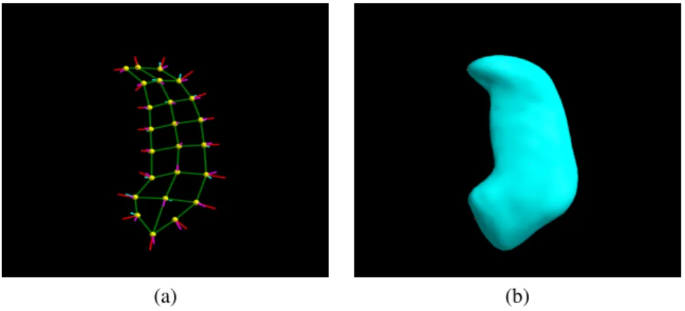
2.1 (a) Skeletal model of a hippocampus s-rep; (b) solid model implied by that s-rep. Yellow spheres are sample points along the skeletal surface. Solid lines extending from these sample points are spoke vectors, which are approximately normal to the boundary surface. Interpolation of a discrete s-rep into a continuous skeleton with a continuous field of spokes forms a continuous s-rep whose spokes completely fill the interior of the object they are

representing. . . 8

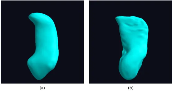
4.1 (a) The solid model of the template hippocampus s-rep; (b) The solid model of a warped

template hippocampus s-rep. . . 14

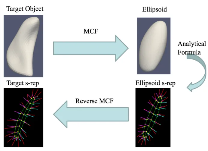
4.2 The illustration of the workflow of the method to obtain the s-rep fitted to the input boundary surface . . . 15

4.3 Skeletal ellipse of an ellipsoid whose principal radii are 23, 8, and 5. The red circles are the sampled internal skeletal points of the skeletal ellipse, and the black boundary curve is the end curve of the true skeletal ellipse. To support the legacy representation of the s-rep, the black ellipse is slightly eroded to the blue ellipse. The black points are the true end skeletal points of the true skeletal ellipse, and these are pulled toward to the eroded ellipse. These pulled points are blue points on the blue ellipse. In this case, the skeletal points are sampled to form5×7grid. After the end skeletal points are sampled along the end curve, the interior skeletal points are uniformly sampled along the blue lines until the

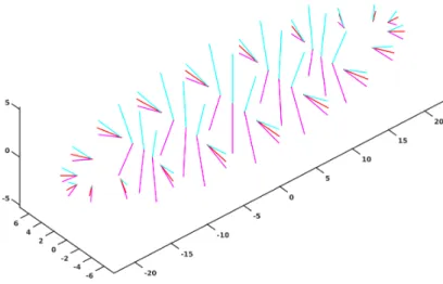
lines intersect the medial curve of the skeletal ellipse,i.e., the horizontal line aty= 0. . . 17 4.4 The computed spokes of the same ellipsoid used in the figure 4.3. The colored lines are

the spokes that are analytically computed using the equations. The cyan and magenta lines denote spokes pointing respectively to the top and bottom side of the ellipsoid. The red

lines point to the crest of the ellipsoid. . . 19

4.5 (a) Fitted s-rep of the hippocampus using the proposed approach; (b) solid model implied

by that s-rep. As can be seen in (a), the lengths of the crest spokes are longer than expected. . . 20

4.6 (a) Fitted s-rep of the hippocampus before the refinement on crest spokes; (b) fitted s-rep of

the hippocampus after the refinement on crest spokes. . . 21

4.7 The histogram of the distances from each base spoke end of the fitted s-rep to the cor-responding object boundary for a case in the population of 6-month olds’ hippocampi.

. . . 22

4.8 The histogram of the mean spoke end distance for the population of hippocampi. . . 23

4.9 The histogram of the distances from each base spoke end of the fitted s-rep to the corre-sponding object boundary for a case in the population of 6-month olds’ caudate nuclei.

. . . 24

4.10 The histogram of the mean spoke end distance for the population of caudate nuclei. . . 25

4.11 (a) Fitted s-rep of a neonate’s left lateral ventricle using the proposed approach; (b) solid

model implied by that s-rep. . . 25

4.12 The histogram of the distances from each base spoke end of the fitted s-rep to the

(12)

5.1 An interpolated skeleton of one of the CN s-reps with the new singular point primitive. The blue arrow seen at the lower left corner of the figure is the directional component of the

singular point primitive. . . 34

5.2 Densely interpolated spokes of the same CN s-rep previously seen in figure 5.1 with the singular point primitive. The magenta vectors denote up spokes, the cyan vectors denote

down spokes, and the red vectors denote crest spokes. . . 35

5.3 The histogram of the average spoke end distance of the augmented CN s-rep fitted to a

population of 6-month olds’ caudate nuclei. . . 37

6.1 Visualizations of the class likelihoods of hippocampi. The empirical histogram of the scalar projection of the non-autistic cases in the training set onto the separation direction is plotted using the blue dotted lines and with the Gaussian probability distribution as the blue solid

curve. Similarly for the autistic class in green. . . 41

6.2 Selected frames from the sequence of the s-reps while walking along the separation direction through the pooled backward mean from the autism class to the non-autism class. Viewing the sequence as a looping movie (available athttps://github.com/jphong89)

(13)

LIST OF ABBREVIATIONS

ASD Autism Spectrum Disorder

B-PDM Boundary Point Distribution Model

CPNS Composite Principal Nested Spheres Analysis

CN Caudate Nucleus

PCA Principal Component Analysis PNS Principal Nested Spheres

PPCA Polysphere Principal Component Analysis DWD Distance Weighted Discrimination GOPs Geometric Object Properties

MCF Mean Curvature Flow

MRI Magnetic Resonance Imaging TPS Thin Plate Spline

(14)

CHAPTER 1: INTRODUCTION

1.1 Overview

The driving biomedical problem of this dissertation is an early diagnosis and detection of Autism Spectrum Disorder (ASD). This work focuses on classifying the autistic from the non-autistic among infants at high familial risk (HR) of ASD based on shapes of hippocampi or caudate nuclei. Among these infants at high risk of ASD, I refer those who are later diagnosed with ASD asHR-ASDand those who are not asHR-Neg. There are two important factors to consider for this shape classification problem:

• A choice of an object model to represent the shape of the hippocampus and the caudate nucleus.

• A choice of a method to learn a classification rule based on shape descriptions of hippocampi and caudate nuclei.

An effective shape classification is difficult because of several challenges associated with each design choice. Firstly, with numerous object models having been proposed in the literature, choosing an object model capable of providing shape descriptions of the object that may be relevant for a classification task at hand is in itself challenging. Secondly, one has to consider whether an object model can be fitted to a set of object segmentation with reasonably good correspondence to obtain a sensitive classification result. Finally, after settling the choice of the object model that satisfies the two aforementioned concerns, choosing a classification method capable of yielding an effective classification rule poses yet another challenge.

In order to effectively discriminate the HR-ASD from the HR-Neg infants based on morphological traits of hippocampi and caudate nuclei, the following properties are necessary for each component of the shape classification.

• An object model needs to

– provide rich localized descriptions of those structures that are sensitive to any subtle morphological difference.

– be fitted to an object segmentation robustly and automatically with good correspondence in the target objects across the sample population.

(15)

• A classification method needs to

– robustly classify cases when the input feature dimension is larger than the sample size.

– account for the fact that GOPs abstractly live on a curved manifold.

This dissertation describes novel methodological contributions in each of these areas. In subsequent sections of this chapter, I first overview the current findings in the driving application problem. Then, I provide details on the intuition behind each of my contributions. Finally, I conclude this chapter with my thesis statement and the organization of the remaining chapters.

1.2 Current Findings on ASD from Neuroimaging Studies

ASD is a neurodevelopmental disorder characterized by a few core symptoms including repetitive behaviors and difficulties in social interaction and communication. ASD manifests very early in life. Previous behavioral studies of ASD show that clinical symptoms may appear as early as 12 months with most infants receiving a diagnosis by the age of 4. This relatively narrow window of birth to age of onset of symptoms provides opportunities to study the underlying neurodevelopmental process of infants with ASD.

Recent longitudinal infant brain imaging studies of infants have yielded many important insights about the developmental process of infants who are diagnosed with autism by the age of 2. Findings include increased cortical gray and white matter volumes, increased amygdala volumes, and atypical neurodevelopmental trajectories (Hazlett et al., 2012; Wolff et al., 2013).

However, not much is known about localized morphological differences ofsubcorticalstructures between the individuals with and without ASD during this early developmental period. In older children there have been a number of studies showing that subcortical structures including the caudate nuclei and the hippocampi are implicated in ASD. This has motivated me to develop classification methods based on local geometric properties of the hippocampus and the caudate nucleus from the perspective of shape classification.

1.3 Common Object Models used in Shape Classification

(16)

causes of the observed difference in volume,e.g., that the volume change is driven by one or more regions of the structures. The localized analysis could yield an important biological insight into the disease.

The Point Distribution Model (PDM) (Cootes et al., 1992) has been a popular object model in shape classifica-tion (Davies et al., 2003). The PDM describes a shape of the object as a tuple of enumerated points usually placed along the boundary of the object. The PDM has several desirable traits such as being easy to create from image data (Davies et al., 2003; Styner et al., 2006) and supporting a localized analysis of the shape of the objects. However, the localized analysis of the shape of the objects with PDMs is still limited due to PDMs only explicitly capturing positional geometrical properties of the objects; therefore, the PDM-based analysis is limited in accurately modeling inter-class shape variations involving a local direction and a local width.

1.4 Skeletal Representations

Skeletal representations describe the shape of an object via a collection of geometric primitives each of which has an associated skeletal position. The s-rep is a skeletal representation whose geometric primitives are vectors called spokespointing to the object boundary from each skeletal position to the object boundary. These spokes provide the rich localized shape properties of the object,i.e., orientation, width, and position. These GOPs are capable of modeling a localized nonlinear inter-class shape difference that may be a useful insight into the classification task.

However, these GOPs,e.g., a set of local directions, are non-Euclidean. Therefore, a classification method has to be chosen carefully because of non-Euclidean nature of the s-rep GOPs: without properly handling the nonlinearity of GOPs, a classification method,e.g., the Support Vector Machine, designed to classify Euclidean data fails to learn a sensible classification rule (Sen, 2008). I use an alternative approach calledEuclideanizationwhere these non-Euclidean s-rep GOPs are properly transformed into a Euclidean feature tuple before learning the classification rule.

1.5 Automatic Generation of S-reps with Good Correspondence

For each target object in the training set, a set of s-reps have been obtained by registering an implied boundary surface of the template s-rep model to each target object boundary. The template s-rep has been deformed to roughly fit each target object boundary via the Thin Plate Spline (TPS) transformation computed based on the correspondence established by Thin Shell Demons (TSD). Then, spokes of each warped template s-rep have been further refined so that the s-rep tightly fits the target object boundary. This process yields a set of fitted s-reps that have a reasonable correspondence in spokes across the set.

(17)

a reasonable correspondence in spokes by warping a single s-rep model to each target object in the set poses another challenge when the chosen template s-rep is not representative of the sample population.

However, an analytical expression of the s-rep is known for an ellipsoid. Thus, the ellipsoid s-rep can be deformed to fit each target object if a mapping between the ellipsoid and the target object is established. I use Mean Curvature Flow (MCF) to obtain the ellipsoidal mapping of the target surface. Then, I apply a deformation that is the inverse of MCF to an ellipsoid s-rep followed by refinements in spokes to the deformed ellipsoid s-rep to obtain a fitted s-rep. Reasonable correspondence in spokes is achieved because ellipsoids are related by scaling each axis of the ellipsoid.

1.6 Extensions of the Discrete S-rep to Model a Singular Point

My driving medical problem requires appropriately capturing geometric properties of the caudate nucleus (CN). The literature reports morphological deviations of the CN between individuals with and without ASD. Especially notable is the association of ASD patients’ restricted and repetitive behaviors with enlargement of the CN’s global volume. However, detailed analysis of the local shape differences of the CN between the two groups is lacking.

The input boundary surface of the CN derived from a medical image,e.g., structural Magnetic Resonance Imaging, tends to have a tapering sharp tail,i.e., a singular point. The singular point on the boundary of the caudate nucleus makes it difficult to represent the structure with an s-rep becuase it causes the skeletal surface to collapse to a point. This degeneracy of the skeletal surface causes a number of issues in modeling the surface geometry of the caudate nucleus.

To address this challenge in modeling neuroanatomical structures with a singular point,e.g., the caudate nucleus, via the s-rep I introduce an additional geometric primitive dedicated to represent the singular point to account for the degeneracy. Then, I extend the current quad-based spoke interpolation method so that the interpolated boundary surface patches areC2_{continuous up to the singular point.}

1.7 Common Classification Methods used in Shape Classification

(18)

as the Euclidean counterparts to the original GOPs; the original non-Euclidean GOPs appear now to be reasonably Euclideanizedfor the Euclidean classification methods.

The shape classification problem is often a High Dimensional Low Sample Size (HDLSS) problem in which the dimension of the input GOPs tuple is larger than the number of available data samples. In the HDLSS classification problem Marron (Marron et al., 2007) has shown that many classifiers,e.g., the Support Vector Machine and the Mean Difference Classifier, lose generalizability due to a phenomenon calleddata piling. To account for this phenomenon in my shape classification tasks, I use Distance Weighted Discrimination, which is designed to learn a generalizable classification rule in HDLSS classification problems.

1.8 Classification based on Temporal Shape Differences

A number of recent psychiatric studies have shown that the brain developmental trajectories of HR-ASD infants noticeably deviate from those of the typically developing infants (Hazlett et al., 2017). However, not much is known about the correlation between ASD and the developmental trajectories of the implicated subcortical structures. This has motivated me to investigate the problem of classifying objects based on growth information as to whether the disease is present. For the early diagnosis of ASD, I have chosen to investigate growth information of hippocampi and caudate nuclei between 6 months and 12 months.

The main task is to accurately encode the growth information as the temporal difference in GOPs of an object between the two time points into the DWD classifier’s feature tuple. This raises a statistical question whether the GOPs of each of the s-rep are analyzed together or separately for PNS. In this work I adopt the latter approach in which the Euclideanized input feature tuple is obtained by taking difference between the s-rep GOPs that are Euclideanized by a common polar system produced from a union of s-reps across the time points and across the classes.

I have evaluated the effectiveness of the temporal difference classification method in two scenarios: 1) ASD classification given the temporal pair of hippocampi of 6-month olds and 12-month olds, 2) ASD classification given the temporal pair of caudate nuclei of 6-month olds and 12-month olds.

1.9 Thesis and Contributions

Thesis: Classification of medically imaged neuroanatomical structures based on their geometric object properties benefits from the following:

1. An object model providing local object width and orientation in addition to positional information

2. An object modeling procedure that efficiently yields geometric correspondence across a population

(19)

The major methodological contributions of this dissertation are as follows:

1. A fully automatic procedure to obtain a set of s-reps fitted to each target object boundary data with reasonably good correspondence in spokes.

2. An extension to the current s-rep modeling framework for appropriately representing an object with a singular point,e.g., the caudate nucleus.

3. A non-Euclidean classification method that uses PNS to obtain the Euclideanized s-rep GOPs on which DWD classifier is trained.

4. A statistical technique to compare different shape classification methods.

5. A non-Euclidean classification method for classifying a temporal difference of s-reps in which the input feature tuple to DWD is formed by taking the difference of the Euclideanized s-rep GOPs for each time point

In addition to the above methodological contributions, I have also accomplished the following engineering contributions:

1. Redesign of the computer representation of the discrete s-rep, which allows modeling objects with different topologies including the spherical (slabular), the quasi-tubular, and the toroidal

2. Integration of Pablo, the main piece of software used to fit and visualize s-reps into 3D Slicer for easier distribution of the s-rep modules to the medical image analysis community

3. Modernization of the s-rep modules

4. Implementation of the module that converts a legacy s-rep into the new s-rep

5. Implementation of the module that visualizes a legacy s-rep in 3D Slicer

(20)

CHAPTER 2: BACKGROUND

In this chapter I lay out background information that is common for each of the subsequent chapters. I first overview object models. Then, I overview statistical methods to understand the shape of an object and then classification methods.

2.1 Object Models

At a high level there are two categories of object models that have been proposed for statistical analysis: continuous, parameterized models modulo parameterization (Kurtek et al., 2012; Jermyn et al., 2012; Bauer et al., 2010, 2012; Durrleman et al., 2014) and discrete models. Due to the discrete models’ strengths in explicitly dealing with localized features, I focus on those models. Among the discrete models are those based on deformations of an atlas (Beg et al., 2005; Miller et al., 2002; Wang et al., 2007), those based on the B-PDM (Cootes et al., 1995; Styner et al., 2006; Davies et al., 2003), and those based on skeletal models (Styner et al., 2004; Yushkevich and Zhang, 2013; Bouix et al., 2005; Schulz et al., 2016). The B-PDM-based models have been the most popular. The skeletal models were designed to add local object width features and local directional features to those provided by PDMs.

I overview the two object models that I compare in this work: the PDM and the s-rep. For each model, I provide

• a brief description of the representation

• a brief description on fitting the object model to a boundary description provided as input

• a brief description of the curved manifold on which shape features of the representation live.

2.1.1 The Point Distribution Model

The PDM is a point tuple for each object in a training set. In the boundary PDM (B-PDM) each example object in the set has a set of enumerated points along its boundary, with points with corresponding index in each object chosen so as to be in correspondence across the training set.

(21)

The PDM GOPs,i.e., a tuple of point coordinates, are often interpreted in two ways: 1) as a point on a flat Euclidean space or 2) as a point on a curved manifold (Kendall, 1984). Consider the B-PDM in the training setPwithnboundary points. By scaling the entire point tuple such that the sum of squares of all the center-of-mass-relative point features has unit value, this can be thought of projecting the point tuple onto the unit hypersphere_S3n−4_{. The dimensionality of} 3n−4comes from the fact that three degrees of freedom were used during alignment and one more degree of freedom was used to normalize the scale to unity. Therefore, as rigorously shown by Kendall in his work (Kendall, 1984), the translationally aligned B-PDM can be represented as a concatenation of this scaling factor and this normalized tuple of points: the B-PDM abstractly lives on the manifoldR+×S3n−4.

2.1.2 The S-Rep

The discrete s-rep is a skeletal discretization of the interior of the object. It consists of a set of points sampled on the skeletal surface, which is a folded surface with the object’s topology, in this dissertation spherical topology, and vectors calledspokesassociated with each of the skeletal points that are approximately normal to the object boundary surface and whose tips are approximately incident to the object’s boundary surface. These spokes explicitly capture local direction and local width information of the object. An example discrete s-rep of a hippocampus can be seen in figure. 2.1.

(a) (b)

Figure 2.1: (a) Skeletal model of a hippocampus s-rep; (b) solid model implied by that s-rep. Yellow spheres are sample points along the skeletal surface. Solid lines extending from these sample points are spoke vectors, which are approximately normal to the boundary surface. Interpolation of a discrete s-rep into a continuous skeleton with a continuous field of spokes forms a continuous s-rep whose spokes completely fill the interior of the object they are representing.

(22)

Then, the deformed reference s-rep is refined to fit tighter to the input object boundary by lengthening or shortening spokes. This process yields a set of s-reps whose spokes are in reasonable correspondence in the training set.

S-rep GOPs,i.e.a tuple of positions, local widths, local orientations, lie on a curved manifold. Consider a discrete s-repswithnspoke vectors andmskeletal points. The set of skeletal points forms a PDM that is aligned such that its center of gravity is at the origin. Additionally, this tuple of centered points is scaled by a factor making the sum of squared distances to the origin to be unity. Therefore, this PDM is described by a tuple of centered points that abstractly lives on the unit hypersphereS3m−4and an associated log-transformed scaling factor. The directional component of each spoke abstractly lives on the unit 2-sphereS2, and the log-transformed associated length component of each spoke lives on the Euclidean spaceR1. Thus, a single discrete s-rep abstractly lives onRn+1×S3m−4× S2n.

2.2 Statistical Methods

I provide brief descriptions of statistical methods commonly used to understand the input shape description of an object. I first overview PCA, the conventional approach. Then, I overview PNS analysis, a variant of PCA to analyze data that live on abstract spheres. I briefly describe CPNS, a statistical analysis technique that is appropriate for analyzing the data that live on a Cartesian product of Euclidean space and hyperspheres. Finally, I finally briefly describe Polysphere PCA (PPCA), a method designed as an extension to PNS to properly understand the correlation of variables in a Cartesian product of hyperspheres,i.e., polysphere.

2.2.1 Principal Component Analysis

Principal component analysis (PCA) is an important statistical method for analyzing Euclidean data. It provides a means of reducing the intrinsic dimension of data by capturing its major modes of variation. PCA has been widely used in the field of medical image analysis and computer vision because descriptions of objects of interest are often high dimensional whereas the important variations can be quite low dimensional. Those modes of variation are often quite illuminating and relevant to the task at hand.

PCA can be understood in terms of a forward or backward procedure. The forward method progressively builds up the dimension of the approximating subspace being fitted to the data, whereas the backward method progressively reduces the dimension of the subspace being fitted to the data. Both approaches yield the same result when the data lie on a Euclidean space. However, GOPs do not lie on a Euclidean space. The backward approach typically yields different results from the forward approach when applied to non-Euclidean data. As noted in (Damon and Marron, 2013), the backward approach is usually more appropriate to analyze those non-Euclidean features.

(23)

best fitting manifold so that the current manifold is the best fitting submanifold of the data in the original dimension. The principal component scores are found by projecting all the data onto the found submanifold.

In contrast, the backward view of PCA progressively reduces the intrinsic dimension of the manifold by removing the component of the least variance from all the data points; at the beginning of each iteration the data is projected onto the submanifold found in the previous iteration, and then the best fitting submanifold is found by minimizing the sum of squared distances of all the projected data.

2.2.2 Principal Nested Spheres Analysis

Principal Nested Spheres (PNS) analysis is a special case of backward PCA on hyperspheres. PNS progressively reduces intrinsic dimension by finding the best fitting subsphereSk−1that is nested in the current hypersphereSk. At each iteration, the data points are first projected onto the subsphere found in the previous iteration; then the fitting is done by minimizing the sum of squared geodesic distances of all the projected data points to the subsphere. Over the training cases PNS will yield a tuple of signed geodesic distances to the best fitting subsphere for each dimension-reduction iteration.

These signed geodesic distances are a Euclideanized form of their spherical counterparts; I call this process Euclideanization. The final result of PNS yields Euclideanized variables and a set of polar systems that provide a means of transformations between the original space and Euclideanized space and vice versa.The dimension 0 point in feature space produced at the end of this iteration is called the backwards mean. (Jung et al., 2012) provides more information on the method.

2.2.3 Commensuration of Spherical GOPs

Suppose the data of interest live on a Cartesian product of a Euclidean space and hyperspheres. Such an instance includes any model described by a combination of GOPs involving PDMs, lengths, directions, and scaling. In this case, PNS is applied independently to each GOP that lives on a hypersphere.

(24)

values are commensurated by multiplying each by their respective geometric mean. Finally, these commensurated log-transformed size features and commensurated spherical GOPs together form a Euclideanized feature tuple.

2.3 Classification Methods

At a high level there are two categories of classification methods: likelihood based methods and separating direction based methods. See (Duda et al., 2012) and (Friedman et al., 2001) for an overview of common existing classification methods. In this dissertation I focus on the methods based on finding an optimal separating direction that points from one class to the other in the feature space because the inter-class shape difference can easily be visualized by interpolating points in the feature space along the separation direction. Given a separation direction, the class label is decided based on scalar projection of data points onto the separation direction.

I concentrate on linear classification methods because 1) in High Dimensional Low Sample Size (HDLSS) setting (when the dimension of data is larger than the sample size), El Karoui demonstrated that there is little value added by Kernel tricks since the kernel method is asymptotically linear method in this setting (El Karoui et al., 2010); 2) I want to gain insights into the driving application problem,e.g.classfying autistic infants from non-autistic infants by directly inspecting features. I especially pay attention to the separating direction vector since large entries in the vector indicate that the corresponding feature is relevant. A good separating direction provides additional information and insight into the data by visualizing the trends between the classes by linearly interpolating and then synthesizing the data in the original feature space along the direction.

2.3.1 Support Vector Machine

The SVM (Cortes and Vapnik, 1995) is a binary classification method that yields a separation direction in the feature space by minimizing the gap between the two classes. SVM then classifies a new example by thresholding the scalar value of the projection of it’s feature tuple onto this direction.

2.3.2 Distance Weighted Discrimination

(25)

CHAPTER 3: MATERIALS

The image dataset which I analyze was acquired from an NIH-funded study of Autism referred to as theInfant Brain Imaging Study(IBIS). I focus on the subset of the participants of this study who are at high familial risk (HR) of ASD because they have an older sibling already diagnosed with ASD. There are 49 infants who were clinically diagnosed with ASD at age 24 months (HR-ASD) and 149 infants who did not meet criteria for ASD (HR-Neg). MRI scans (Siemens 3T TIM Trio scanners, T1-weighted imaging at1.0×1.0×1.0mm voxel resolution) were acquired while infants were naturally sleeping. The infants were scanned longitudinally at the age of 6 months, 12 months, and 24 months. The MRI scans were aligned to a common coordinate system. Subcortical structures were automatically segmented from the aligned MRI scans (Wang et al., 2014). Details on the original MRI dataset can be found in (Hazlett et al., 2017; Wolff et al., 2015; Lewis et al., 2014).

Bilateral hippocampi and the caudate nuclei are expected to be associated with ASD. However, I fitted the s-rep to the left hippocampus and the left caudate nucleus for method development.15records for the HR-ASD at 6-months and6records for the HR-Neg were not available to us at the time of the analysis. Thus, the dataset we use in this study consists of 34 autistic infants and 143 non-autistic infants.

(26)

CHAPTER 4: AUTOMATIC GENERATION OF CASE-SPECIFIC S-REPS

4.1 Introduction

The s-rep has been shown to be a powerful shape representation in various statistical shape analysis tasks including hypothesis testing (Schulz et al., 2016), classification (Hong et al., 2016), shape probability distribution estimation, and segmentation (Vicory, 2016). For these tasks it is important that the set of s-reps have good correspondence in spokes across the set to yield meaningful statistical insights related to the morphology of the target object in the sample population. Tu et al. (Tu et al., 2018) proposed an entropy-based method to improve the s-rep spoke correspondence. However, for a set of s-reps of even moderate size (e.g.,30cases) the method cannot be applied because of its prohibitive computational cost.

As mentioned in section 2.1.2, one approach to establish the s-rep correspondence across the set is to warp a single template s-rep to fit each target object surface. However, using a single template model as a basis of the spoke correspondence tends to cause difficulties for the s-rep fitting process. This approach often yields a set of s-reps that contain geometric artifacts,e.g., creases and folds, on the boundary surface implied by the fitted s-reps as can be seen in figure 4.1. These artifacts arise because of 1) the difficulty in finding the appropriate template s-rep that is representative of the population of interest and 2) the difficulty in estimating the deformation that respects the skeletal geometry of the target object.

I argue that the following properties are desirable for the optimal template s-rep:

1. It is case-specific.

2. It is obtained from an analytical expression.

3. The correspondence across the cases in the set can be achieved with a simple transformation.

In this chapter I present a novel method to automatically generate a set of fitted s-reps with reasonably good correspondence across the cases. The method works as follows:

1. Deform a target object surface to an ellipsoid via Mean Curvature Flow (MCF).

(27)

(a) (b)

Figure 4.1: (a) The solid model of the template hippocampus s-rep; (b) The solid model of a warped template hippocampus s-rep.

3. Deform the ellipsoid s-rep back to the original object via reverse MCF transformations.

The remainder of this chapter is organized as follows. First, I provide a brief description of MCF and the Thin Plate Splines (TPS). Then, I describe the method in detail. I demonstrate that the method is effective at generating s-reps for 6-month old infants’ hippocampi, caudate nuclei, and neonates’ lateral ventricles. Finally, I conclude this chapter with discussion.

4.2 Background

4.2.1 Mean Curvature Flow

Mean Curvature Flow (MCF) is a geometric flow method in which the input surface evolves along the surface normal proportional to the mean curvature of the surface. MCF is mathematically defined as the following:

∂

∂tS(x, t) =H(x, t)N(x, t)

S(x,0) =S0(x)

(28)

Hat each vertexx∈V is estimated as the average of dihedral angles of the triangles that share the vertexx. A more

extensive introduction of MCF is available in (Mantegazza, 2011).

4.2.2 Thin Plate Splines

Thin Plate Splines (TPS) has been commonly used in non-rigid image registration given two sets of landmarks. The method generates a full 3D deformation field by interpolating the displacement of the landmarks. TPS is not guaranteed to produce a diffeomorphic transformation; it can produce folds within the deformation field. However, this can be prevented if the displacement vectors are short enough. A more comprehensive reference on using TPS for image registration is available in (Bookstein, 1997).

4.3 Method for Automatic S-rep Fitting

Figure 4.2: The illustration of the workflow of the method to obtain the s-rep fitted to the input boundary surface

(29)

direction of the MCF so that the s-rep will roughly fit the original boundary data. I provide details of each step of the method.

4.3.1 Applying MCF to the Deforming Surface

I iteratively apply MCF to the triangle mesh of the object derived from the image data. In order to improve the numerical stability in computing the discrete mean curvature at each vertex, at each iteration of the process prior to applying MCF I apply Taubin smoothing (Taubin, 1995); as a side effect, the smoothing yields more regularly shaped triangles.

4.3.2 Determining if the Deforming Surface is Ellipsoidal

After I apply MCF to the mesh, I examine the second moment of the mesh to see if it is ellipsoidal. The second moments matrix of the mesh is computed as the following.

      P ix 2 i P ixiyi

P ixizi P

iyixi P

iy 2 i

P iyizi P

izixi Piziyi Pizi2      

wherexi, yi, ziare coordinates ofithboundary vertex relative to the center of mass of those vertices.

The eigendecomposition of the matrix yields the three principal axes and spread of the data along each principal axis. Using the result of the eigenanalysis, I derive the analytical expression of the best-fitting ellipsoid for the mesh. Then, I compute absolute value of shortest distance between each vertex of the deforming mesh and the best fitting ellipsoid. If the95%quantile of the distance is less than a threshold, I conclude that the current surface is ellipsoidal enough. I save all the intermediate deforming meshesSii = 1,2, ..., nfor later computation of the reverse MCF transformation.

4.3.3 Obtaining the S-rep of the Best-Fitting Ellipsoid

Once the surface deformed by MCF is ellipsoidal enough, the best-fitting ellipsoid’s s-rep is analytically derived as the following:

1. Sampling the skeletal surface of the ellipsoid

(30)

Given the principal radiirx, ry, rzof the ellipsoid that is aligned so that the radii are ordered asrx> ry> rz, the skeletal sheet of the ellipsoid is an ellipse that satisfies the following equation:

x2

m2 x

+ y 2

m2 y

≤1 (4.1)

wheremx=r 2

x−r

2

z

rx , my =

r2

y−r2z

ry .

Figure 4.3: Skeletal ellipse of an ellipsoid whose principal radii are 23, 8, and 5. The red circles are the sampled internal skeletal points of the skeletal ellipse, and the black boundary curve is the end curve of the true skeletal ellipse. To support the legacy representation of the s-rep, the black ellipse is slightly eroded to the blue ellipse. The black points are the true end skeletal points of the true skeletal ellipse, and these are pulled toward to the eroded ellipse. These pulled points are blue points on the blue ellipse. In this case, the skeletal points are sampled to form5×7grid. After the end skeletal points are sampled along the end curve, the interior skeletal points are uniformly sampled along the blue lines until the lines intersect the medial curve of the skeletal ellipse,i.e., the horizontal line aty= 0.

Once the analytical expression of the skeletal ellipse is obtained, I need to produce a sampled skeleton in a way that supports classification on the set of fitted s-reps. To do this, I samplen1points along the major axisu1andn2 points along the minor axisu2of the ellipse to generate a grid of skeletal points on the ellipse. Bothn1andn2are odd numbers. In our own research group the choice ofn1andn2is made on the basis of level of detail of the surface geometry that we deem necessary for a statistical task on a given population of an object. Please refer to chapter 3 of (Vicory, 2016) to learn how the number of sampled skeletal points affects the level of detail on the surface geometry. In this dissertation I won’t discuss this matter further.

(31)

lastn1points; the interior points are sampled until they intersect with the medial curve of the ellipse,i.e., the horizontal line aty= 0. Figure 4.3 shows an example of a sampled skeletal ellipse.

Given a grid of sampled skeletal points on the skeletal ellipse, I need to compute the ellipsoid’s spoke vectors for all the skeletal points. I compute spoke vectors by finding the ellipsoid’s boundary points implied by the spokes. Letq

be a boundary point implied by a spoke andpbe a skeletal point to which the spoke is attached. Using the spherical parametrization of the ellipsoid, the coordinate ofqis(rxcos (θ) cos (φ), rysin (θ) cos (φ), rzsin (φ)). According to the skeletal geometry, a valid spoke vectorpq~ satisfies the following property:qlies on a bitangent sphere centered atp

maximally contained within the ellipsoid. Therefore, the unit vector _|pq_pq~_~_|is the surface normal of the ellipsoid atq. I need to computeθandφofqthat satisfy the skeletal geometric constraint to compute the spoke vector. Given that the skeletal pointp= (x, y,0),θandφare computed as the following:

tan (θ) = ymx

xmy

cos (φ) = q

y2_m2

x+x2m2y

mxmy

(32)

Figure 4.4: The computed spokes of the same ellipsoid used in the figure 4.3. The colored lines are the spokes that are analytically computed using the equations. The cyan and magenta lines denote spokes pointing respectively to the top and bottom side of the ellipsoid. The red lines point to the crest of the ellipsoid.

By mathematical definition the skeletal points on the end curve of the ellipse should have only one spoke that points to the crest of the ellipsoid. However, the true crest spokes are pulled to be attached to the nearest end skeletal points of the eroded skeletal ellipse to support the legacy computer representation of the s-rep.

For the purpose of classification I need to obtain a set of s-reps fitted to the given population of an object with reasonable spoke correspondence. In order to ensure reasonable spoke correspondence of the fitted s-reps, I need to establish spoke correspondence among ellipsoid s-reps. Application of MCF on different cases in the population often yields ellipsoid s-reps of different principal radii. Different ellipsoids can be related with each other by simple scalings along the principal axes if the following assumptions hold:

1. Objects in the population are rotationally aligned

2. The converged ellipsoids have distinct principal radii, which can be used to establish correspondence among the axes of the ellipsoids.

(33)

4.3.4 Transforming the Ellipsoid S-rep back to the Original Surface

Given a case-specific ellipsoid s-rep, I need to deform the ellipsoid s-rep to match the original object boundary at the spoke ends. To accomplish this, I deform the skeletal points and the spoke ends of the best-fitting ellipsoid s-rep first to the approximate ellipsoid and then in reverse direction of the MCF. I compute the deformation as a series of the TPS transformations. I treat the intermediate surfaces’ triangle mesh vertices saved throughout the MCF as the landmarks to compute each successive TPS transformation:Ti_:_Si_→_Si−1_where_Ti_denotes_i_{-th transformation,}_Si andSi−1_denote_i_{-th and}_i₋_{1-th surfaces from MCF. Figure 4.5 is an example of the s-rep fitted to one of hippocampi} in the dataset.

(a) (b)

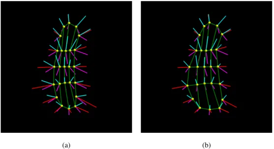
Figure 4.5: (a) Fitted s-rep of the hippocampus using the proposed approach; (b) solid model implied by that s-rep. As can be seen in (a), the lengths of the crest spokes are longer than expected.

Because the reverse MCF deformation is computed purely based on boundary points, some skeletal geometric properties are not properly propagated throughout the deformation. One such property is the length of the crest spokes. For example, in figure 4.5 many of the crest spokes are too long. This is problematic for the following two reasons:

1. It narrows the quadrilaterals formed by neighboring skeletal points, which can cause numerical instability for spoke interpolation. It can even cause the skeletal surface to almost collapse to a curve, which can give wrong interpretation about the topology and skeletal geometry of the object.

2. It yields a too small curvature at the end of the crest spoke.

(34)

4.3.5 Refining Skeletal Geometric Constraints of the Initial Fitted S-rep

To mitigate the problem of the initial fitted s-rep having unexpectedly longer crest spokes, I place an additional constraint when computing the final TPS so that the computed deformation respects the curvature. To achieve this, for the final TPS of the reverse MCF deformation I add an additional pair of landmarks at each skeletal point on the end curve of the skeleton. The pair’s target landmarks are the crest implied loci of the end skeletal points.

The target landmarks need to be the radius of the curvature away from the crest of the object along its normal. In order to estimate the radius of the curvature, I use the implied boundary of the initially fitted s-rep. I compute the radius of the curvature of a curve that spans across the spokes of the end skeletal points; I fit a cubic B-spline to boundary points obtained from spokes interpolated from the top spoke to the crest spoke and from the crest spoke to the bottom spoke.

However, I have found the estimated radius of curvature to be an underestimate of the desired length. In contrast, the current crest spoke length based on boundary points alone is an overestimate of the desired length. As a result, I take the geometric mean of the estimated radius of curvature and the current crest spoke length as a reasonable estimate for the desired crest spoke length.

Finally, I recompute the final TPS transformation with the additional pair of landmarks so that the final warped s-rep has more appropriate crest spoke length. Figure 4.6 shows before and after the refinement on the crest spokes of the same hippocampus s-rep seen in figure 4.5.

(a) (b)

Figure 4.6: (a) Fitted s-rep of the hippocampus before the refinement on crest spokes; (b) fitted s-rep of the hippocampus after the refinement on crest spokes.

(35)

4.4 Results

In this section I present several results of applying the proposed method to automatically obtain an s-rep of an object. I investigated the method’s effectiveness in producing a set of s-reps for 6-month olds’ hippocampi and caudate nuclei; for both the hippocampus and the caudate nucleus, there are 34 austic cases and 143 non-autistic cases. In addition, to assess the method’s applicability to thin objects, I applied the method to obtain s-reps for 3 neonates’ lateral ventricles.

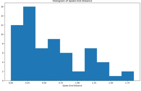
In order to get a sense on the accuracy of the proposed method, I examine how well the fitted s-rep matches the original object boundary. I examine the distribution of the distance from each spoke end of the fitted s-rep to the original object boundary; the distance is measured in voxel units where the resolution of the image is supersampled to 0.05×0.05×0.05mm. Figure 4.7 shows the histogram of the distances of a case in the population of 6-month olds’ hippocampi.

Figure 4.7: The histogram of the distances from each base spoke end of the fitted s-rep to the corresponding object boundary for a case in the population of 6-month olds’ hippocampi.

(36)

In order to assess the quality of s-reps fitted to the population, I examine the distribution of the mean spoke end distances of each hippocampus s-rep. Figure 4.8 shows the histogram of the mean spoke end distances.

Figure 4.8: The histogram of the mean spoke end distance for the population of hippocampi.

From figure 4.8 the mean spoke end distance is less than a voxel; therefore, the fitted s-reps on average achieve sub-voxel accuracy in matching the original object boundary. The mean and the maximum of the mean spoke end distance are0.73voxel widths and1.14voxel widths respectively.

(37)

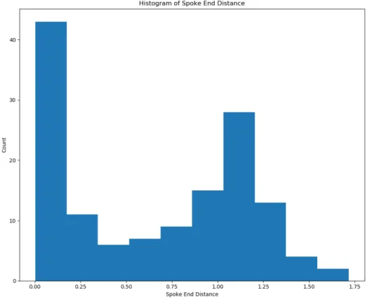
Figure 4.9: The histogram of the distances from each base spoke end of the fitted s-rep to the corresponding object boundary for a case in the population of 6-month olds’ caudate nuclei.

Figure 4.10 shows the distribution of the mean spoke end distances of the fitted caudate nucleus s-reps. The mean and the maximum of the mean spoke end distance are0.65voxel widths and0.70voxel widths respectively.

In order to evaluate the method’s general applicability in producing an s-rep of an object other than the hippocampus and the caudate nucleus, I applied the method to obtain the s-rep of the lateral ventricle of a neonate. Thin structures like the lateral ventricle have been challenging to adequately model with s-reps. Also, the lateral ventricle is a more strongly curving structure than both the hippocampus and the caudate nucleus. Figure 4.11 shows the s-rep fitted to one of the three lateral ventricles I fitted; in each one the fitted s-rep is capable of producing a smooth boundary, which indicates that the s-rep adequately represents the lateral ventricle’s surface geometry.

Figure 4.12 shows the distribution of the chosen lateral ventricle s-rep’s spoke end distances with the mean and the maximum being0.54and1.40voxel widths respectively.

(38)

Figure 4.10: The histogram of the mean spoke end distance for the population of caudate nuclei.

(a) (b)

Figure 4.11: (a) Fitted s-rep of a neonate’s left lateral ventricle using the proposed approach; (b) solid model implied by that s-rep.

(39)

Figure 4.12: The histogram of the distances from each base spoke end of the fitted s-rep to the corresponding object boundary for a neonate’s lateral ventricle.

produce an s-rep for the rather complicated shaped mandible. Throughout MCF, the vertices of the deforming meshes get clustered causing numerical instability in computing the reverse MCF deformation.

4.5 Discussion and Conclusion

In this chapter I have presented a novel method to automatically generate a set of fitted s-reps with reasonably good spoke correspondence by first deriving a case-specific ellipsoid s-rep via MCF and then applying the deformation to warp the ellipsoid s-rep to match the original object boundary. It has produced a set of the reasonably well fitted s-reps for hippocampi and caudate nuclei in 6 months olds. In addition, the method produces a reasonably well fitted s-rep for the lateral ventricle that the previous s-rep fitting approach often fails to produce a satisfactorily fitted s-rep.

(40)

an ellipsoid. I speculate that employing different geometric flows,e.g., Wilmore Flow or Ricci Flow, together with remeshing can address these problems.

The fitted s-reps can be further improved in three aspects. First, the length of the spokes can be adjusted to tighten the s-rep’s fit to the original object boundary. Secondly, the spoke directions can be adjusted to be more approximately orthogonal to the original object boundary. Lastly, different means of mapping the ellipsoid to the original object can be explored; especially, learning-based surface registration methods to learn reverse MCF mappings may improve performance.

(41)

CHAPTER 5: EXTENSIONS OF THE S-REP TO MODEL A SINGULAR POINT

5.1 Introduction

In the literature morphological deviation in the caudate nucleus (CN) between individuals with and without ASD has been reported (Wolff et al., 2013; Hazlett et al., 2012). Especially notable is the association of a core symptom of ASD,i.e., restricted and repetitive behavior, with enlargement of the structure’s global volume. However, detailed analysis on local morphological differences of the CN between the two groups is lacking.

The CN is a subcortical structure with a long tail that forms the dorsal striatum together with the putamen. However, the segmentation of the CN tends to be cut off at the tail due to a low contrast between the CN’s tail and the surrounding tissue.

As it currently stands, an s-rep has difficulties in modeling an object with a singular point,e.g., the CN. The singular point on the boundary of the object causes the skeletal surface to collapse to a point; this degeneracy of the skeletal surface causes a number of issues in modeling the surface geometry of the object of interest. In addition, the s-rep cannot properly model the singular point because of the s-rep’s hard constraint that no spoke can cross another; this hard constraint is too hard to maintain at the singular point.

To address this challenge in modeling neuroanatomical structures with a singular point via the s-rep, I introduce an additional geometric primitive dedicated to represent the singular point to account for the degeneracy of the skeletal surface. Then, I extend the current quad-based spoke interpolation method so that the interpolated boundary surface patches areC2continuous up to the singular point.

This chapter is organized as follows. First, I overview the underlying mathematics of the s-rep and the current quad-based spoke interpolation method. Then, I describe the method in detail as follows:

1. The geometric primitive to represent the singular point

2. The extension of the current spoke interpolation method to obtain the continuous s-rep

3. The method to properly Euclideanize a population of the s-reps augmented with the primitive

(42)

5.2 Background

In this section I briefly overview background necessary to understand the proposed extension to the s-rep to model the singular point and its interpolation into a continuous s-rep. First, I overview the mathematical definition of a continuous s-rep. Then, I overview a geometric interpolation method to obtain an interpolated s-rep from a discrete legacy s-rep.

5.2.1 Mathematics of S-reps

A 3D, continuous s-rep is defined by two parametric functions:

• p(u1, u2): a 2D, non-branching skeletal surface

• S(u1, u2): a field of non-crossing spokes emanating fromp(u1, u2); each spoke approximately orthogonally intersects the object boundary.

S(u1, u2)can be viewed as a product of two additional parametric functions:U(u1, u2), a unit normalized vector field ofS(u1, u2)andr(u1, u2), a scalar field of |S(u1, u2)|, the distance fromp(u1, u2)to the object boundary along theU(u1, u2). Accordingly, a point on the implied boundary of the s-rep can be expressed asB(u1, u2) =

p(u1, u2) +r(u1, u2)U(u1, u2).

This continuous s-rep is discretized to support various statistical tasks,e.g., classification. The legacy discrete s-rep used in this work has a skeletal surface which is discretely sampled by a grid ofm×npoints. From each point either two (on the interior) or three (along the fold curve of the skeleton) spokes emanate from the skeleton.

However, it is necessary to ensure that s-reps properly model the surface geometry of target objects prior to the classification. To assess how well the fitted s-rep matches the original object boundary, I need to be able to quantify the difference between the implied boundary of the s-rep and the object boundary. The implied boundary is obtained by continuously interpolating the base spokes of the s-rep.

5.2.2 Mathematics of Spoke Interpolation

Interpolating a discrete s-rep into a continuous s-rep is divided this into 1) a skeletal surface interpolation operation and 2) a spoke interpolation on the interpolated skeletal surface. The skeletal surface interpolation method uses standard polynomial-based methods.

(43)

Let the skeletal surface be parameterized by(u1, u2), where both parameters are integers at the corners of a quadrilateral in the grid on which the discrete s-rep is specified. Thus, the discrete s-rep gives bothrand U at these quadrilateral corners. Consider interpolation of the spoke directionsU at any pointp(u1, u2)within any grid quadrilateral on the skeletal surface. Our plan for interpolation ofris based on a 2nd-order Taylor series, for which we need not only the spoke directions U but also their first and second order derivative valuesUui andUuiui for

i= 1,2at arbitrary points in the quadrilateral. Spoke directions live on the unit 2-sphereS2. Thus, the sort of finite difference calculations that must be used in order to computeU at our discrete skeletal points should be done on the sphere. These calculations are done by representing the discrete spokesU as unit quaternions and thus its derivatives with respect touias derivatives on the sphere. Using these derivatives, Vicory applies thesquadmethod (Shoemake, 1987) of interpolating quaternions to estimate the spoke directionU at an arbitrary point interior to a quadrangle of discrete points by fitting Bezier curves to the quaternions on the surface of the sphere. This approximation allows the computation of not only theU values but also their directional derivatives of both first and second order in eitheru1or

u2.

Given the ability to evaluateUand its derivatives in a quadrilateral, we need to interpolate thervalues in a way consistent with skeletal geometry. Spokes can be writtenS=rU. The derivatives of the spoke at a skeletal locationp

with respect to a step in directionvin either of the two orthogonal directionsu1oru2must followSv=rUv+rvU, from which it follows thatrv=Sv·U. Also,Svv·U = (Sv)v·U =rvv+rU. From this a Taylor series in the length

dof a small step in directionvfrom a skeletal positionptogether with three forward distance derivative approximations yields the following expression.

r(p+dv) =1

2(S(p) +S(p+ 2dv)) (5.1)

Because the same mathematics works using a Taylor series in the backwards direction about

p+ 2dv, for symmetry and to reduce approximation error the results of the two versions should be averaged, yielding the final formula as

r(p+dv) =U(p+dv)·

₁

2(S(p) +S(p+ 2dv))

−d

2

4 (S(p)·Uvv(p) +S(p+ 2dv)·Uvv(p+ 2dv))

(5.2)

(44)

point within the quadrilateral. Finally, since the method gives different results when you apply it first inu2and then in

u1, we compute using both orders and average the results.

At a skeletal fold, the skeletal surface’s lack of smoothness prevents the direct application of the aforementioned method. We solve this problem by dilating the fold curve into a tube of very narrow radius, treating the spoke at the curve as its value at the place it intersects the tube, and then using the method for smooth surfaces to compute the continuation of the spoke to the object boundary.

5.3 Method for Modeling the Singular Point

As previously mentioned, the current s-rep modeling framework is limited in geometrically modeling an object with a singular point because of the degenerate skeleton and the hard constraint of non-crossing spokes. I address this challenge as follows:

1. I introduce a new geometric primitive to represent the singular point.

2. I modify the current interpolation method to produce interpolated s-reps with the new primitive.

3. I introduce a statistical method to analyze a set of s-reps that contain the new primitive.

5.3.1 Singular Point Primitive

The radius of the curvature at the singular point of the CN is zero, which yields a skeletal surface that not only collapses to a point but also forms a cusp at the CN’s boundary. Based on this observation, I explicitly represent the singular point as a point on the boundary with a direction.

5.3.2 Proposed Interpolation Method

(45)

5.3.2.1 Skeleton Interpolation

In this section I describe how to construct a smooth, continuous skeleton up to the singular point. I construct the skeleton from a smoothly varying series of non-crossing curves. As shown in figure 5.1, these curves emanate from the respective positions interpolated along the base skeleton’s end curve and converge to the singular point in its designated direction. I construct each individual curve as follows:

1. Interpolating the curve’s starting point along the base skeleton’s end curve

2. Determining an emanating direction of the curve at the starting point

3. Limiting the speed along that direction to enforce the non-crossing property of the curve

A starting point of each curve is first interpolated along the base skeleton’s end curve. The point is interpolated from a cubic Hermite spline fitted to two adjacent skeletal points between which the point lies in s-rep’s parametric space. Given the same parametrization of the skeleton in(u1, u2), let the interpolated starting point along the end curve bep(u∗₁, u0

2), and let the two adjacent skeletal end points along the end curve bep(ui1, u02)andp(u i+1

1 , u02). Hermite interpolation requires 4 control values: two positional values of each point,p(ui

1, u02)andp(u i+1

1 , u02), and two vectors

pu1(u i

1, u02)andpu1(u i+1

1 , u02); the partial derivatives are computed via finite differences. The vectorHccontaining these control values is

Hc= p ui1, u 0 2

, p ui+1₁ , u0₂

, pu1 u i 1, u

0 2

, pu1 u i+1 1 , u

0 2

LetH(x) = (H1(x), H2(x), H3(x), H4(x)), where theHis are the cubic Hermite spline basis functions:

H1(x) = 2x3−3x2+ 1

H2(x) =−2x3+ 3x2

H3(x) =x3−2x2+x H4(x) =x3−x2

(5.3)

Then,p(u∗

1, u02)can be computed by the following equation:

p(u∗₁, u0₂) =H(u∗₁−ui₁)·H_c>

The same spline-based interpolation strategy is used to obtain the curve that originates fromp(u∗₁, u0

2)and converges to the singular point in the designated direction. As previously noted, the interpolation requires two positional values as well as the two vectors tangent to the curve atp(u∗₁, u0

(46)

The idea is to specify the emanating vectors at the discrete skeletal end points and to do so in a way that allows the emanating vectors at intermediate points to be interpolated via quaternion splines. Given the two adjacent end skeletal pointsp ui

1, u02

andp ui+1₁ , u0 2

between which the starting point lies, the direction of the vector is obtained from a quaternion-based interpolation ofpu2 ui1, u02

andpu2 ui+11 , u02

. These partial derivatives are computed via finite differences.

Given the direction of the vector atp(u∗₁, u0

2), I need to decide the speed along the emanating vector so that the produced curve does not cross other curves. Two curves at two distinct interpolated starting points can cross each other when the emanating vectors are facing each other; however, the crossing can be prevented if the speeds along the respective vectors are constrained to be less than the half of the arc length between the two starting points. A similar intuition is often used in image registration when obtaining a dense displacement field from a sparse set of displacement vectors. Based on this observation, I constrain the magnitude of emanating vectors for thep(u∗1, u02)s as follows:

1. Finding the minimal arc length of the two adjacent base skeletal end points; let this value beLmin

2. Finding the maximal partial derivative of the skeleton at the discrete skeletal end points with respect tou2; let this value beSmax

3. Computing a scale factorγas a ratio of Lmin

2 toSmax

4. Adjusting the speed along the emanating directions at the discrete skeletal end points byγ

5. Interpolating the speed along the intermediate emanating vectors

(47)

Figure 5.1: An interpolated skeleton of one of the CN s-reps with the new singular point primitive. The blue arrow seen at the lower left corner of the figure is the directional component of the singular point primitive.

5.3.2.2 Spoke Interpolation

In this section I describe how to obtain a continuous s-rep from a discrete s-rep given the singular point primitive. I construct a dense vector field of spokes on the skeleton by interpolating spokes along each skeletal curve. As shown in figure 5.2, spokes on each curve smoothly vary from the respective spokes interpolated along the base skeleton’s end curve to the specified direction at the singular point. The spoke vectors along each skeletal curve are obtained as follows:

1. Interpolating the initial spoke along the base skeleton’s end curve

2. Interpolating the desired spoke from the initial spoke to the singular point.

An initial spoke is first interpolated along the base skeleton’s end curve. Let the initial spoke beS u∗1, u02

whose tail position is the interpolated end skeletal pointp u∗1, u02

. The spoke directionU u∗1, u02

is estimated from a quaternion-based interpolation. The spoke lengthr u∗

1, u02