Physically-based simulation of ice formation

(1)

by

Theodore Won-Hyung Kim

A dissertation submitted to the faculty of the University of North Carolina at Chapel Hill in partial fulfillment of the requirements for the degree of Doctor of Philosophy in the Department of Computer Science.

Chapel Hill 2006

Approved by Advisor: Ming C. Lin Reader: Mark Foskey Reader: Anselmo Lastra Reader: David Adalsteinsson

(2)

(3)

c ° 2006

(4)

(5)

ABSTRACT

THEODORE WON-HYUNG KIM: Physically-Based Simulation of Ice Formation.

(Under the direction of Ming C. Lin.)

The geometric and optical complexity of ice has been a constant source of wonder and inspiration for scientists and artists. It is a defining seasonal characteristic, so modeling it convincingly is a crucial component of any synthetic winter scene. Like wind and fire, it is also considered elemental, so it has found considerable use as a dramatic tool in visual effects. However, its complex appearance makes it difficult for an artist to model by hand, so physically-based simulation methods are necessary.

In this dissertation, I present several methods for visually simulating ice formation. A general description of ice formation has been known for over a hundred years and is referred to as the Stefan Problem. There is no known general solution to the Ste-fan Problem, but several numerical methods have successfully simulated many of its features. I will focus on three such methods in this dissertation: phase field methods, diffusion limited aggregation, and level set methods.

Many different variants of the Stefan problem exist, and each presents unique chal-lenges. Phase field methods excel at simulating the Stefan problemwith surface tension anisotropy. Surface tension gives snowflakes their characteristic six arms, so phase field methods provide a way of simulating medium scale detail such as frost and snowflakes. However, phase field methods track the ice as an implicit surface, so it tends to smear away small-scale detail. In order to restore this detail, I present a hybrid method that combines phase fields with diffusion limited aggregation (DLA). DLA is a fractal growth algorithm that simulates the quasi-steady state, zero surface tension Stefan problem, and does not suffer from smearing problems. I demonstrate that combining these two algorithms can produce visual features that neither method could capture alone.

(6)

(7)

ACKNOWLEDGMENTS

First, I want to thank my advisor, Ming Lin. If not for her physically-based modeling course, I would not have found the seed of an idea that was later expanded into this dissertation, and if not for her subsequent patience and support, I would not have been able to develop and expand these ideas into their current form. Without her, this dissertation would simply not exist. I would also like to thank all of my committee members, David Adalsteinsson, Mark Foskey, Anselmo Lastra, and Dinesh Manocha, for their patience and understanding, especially since this dissertation took a bit longer than I had originally predicted.

I would also like to thank my parents and brother for their constant support through-out my entire graduate career. Maybe this year, for the first time in five years, I won’t spend Thanksgiving and Christmas cloistered away, working on a paper.

Without my friends in Chapel Hill, Karl Gyllstr¨om, Andrew Leaver-Fay, and Younoki Lee, I am sure that burnout would have brutally truncated my graduate career long ago. A special thanks to Younoki for her endless supply of delicious imitation crab salad. I also want to thank my undergraduate roommate, Jeremy Kubica. Perhaps this memory is apocryphal, but first semester freshman year, you said you wanted to work in robotics, and I said I wanted to do graphics. If you’re reading this, it means we now have PhDs in these fields.

My summer internships at Rhythm and Hues Studios in Los Angeles taught me what industrial-strength code and movie production pipelines looks like, for which I have to thank Jubin Dave and zuzu Spadaccini. You gave me an invaluable professional experience, and more importantly, your friendship.

(8)

(9)

LIST OF FIGURES

1.1 Taxonomy of Snowflakes . . . 3

1.2 Snowflake Photographs . . . 4

1.3 Combination of plate and dendritic growth . . . 4

1.4 Photograph of frost . . . 5

1.5 Icicles On a Fountain . . . 6

1.6 One-sided Stefan problem . . . 9

2.1 von Koch Snowflake . . . 16

3.1 Closeup of ice on a stained glass window . . . 38

3.2 Phase field system pipeline . . . 39

3.3 Cross-section of phase fields . . . 41

3.4 Comparison of phase field snowflakes to real snowflakes . . . 45

3.5 Phase field controls . . . 53

3.6 Border extraction operation . . . 57

3.7 Structuring Elements . . . 58

3.8 Results of modified erosion operator . . . 58

3.9 Skeletonization structuring elements . . . 59

3.10 Results of skeleton and border operations . . . 60

(16)

3.12 Sharpening Results . . . 61

3.13 Lilypad ice growth . . . 65

3.14 Ice ring growth . . . 69

3.15 Ice growth on a window panel . . . 70

3.16 Ice growing on a red stained glass window . . . 71

3.17 Ice growing on a stained glass window . . . 72

3.18 Light refracting through a stained glass window . . . 73

4.1 A microscopic view of the three stages of freezing . . . 76

4.2 Grid anisotropy in diffusion limited aggregation. . . 79

4.3 Stencils and initial conditions for DBM . . . 82

4.4 Comparison of DBM and DLA . . . 84

4.5 Finite difference stencils for a hexagonal grid . . . 88

4.6 A 4-armed dendrite growing in a flow . . . 91

4.7 Phase fields with and without diagonal terms . . . 93

4.8 Frosty ice forming on a chilled glass . . . 102

4.9 Ice Accumulated on a car . . . 103

4.10 Frost forming on a window . . . 104

4.11 Comparison to hybrid algorithm to DLA and phase fields . . . 105

4.12 Validation of hybrid algorithm against a photograph . . . 106

(17)

5.1 2D slice of parabolic coordinate system . . . 115

5.2 Ray traced icicle star . . . 126

5.3 BSSRDF icicle star . . . 127

5.4 Experimental validation of thin-film Ivantsov parabola . . . 130

5.5 Icicle star . . . 132

5.6 Icicle star forming . . . 133

5.7 A freezing fountain . . . 134

(18)

(19)

LIST OF TABLES

2.1 Symbols for the Makkonen model . . . 23

3.1 Phase field constants . . . 43

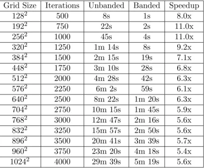
3.2 Banded vs. Unbanded Performance . . . 50

3.3 CPU vs. GPU performance . . . 52

4.1 Phase field performance over different resolutions . . . 96

4.2 Timing results for simulation . . . 97

5.1 Table of icicle symbols. . . 117

(20)

(21)

Introduction

Many years later, as he faced the firing squad, Colonel Aureliano Buend´ıa

was to remember that distant afternoon when his father took him to discover

ice.

– Gabriel Garcia Marquez, One Hundred Years of Solitude

Ice formations are one of the most memorable and visually arresting phenomena in nature. On cold mornings, branching frost patterns can be found on sidewalks, window panes, and car windshields. No winter scene would be complete without icicles dangling from tree branches and rooftops. These formations are interesting because they exhibit a high degree of geometric and optical complexity. As the old adage says: “No two snowflakes are alike.” The same could pedantically be said about any collection of objects, but the saying rings true for snowflakes because they span such a wide variety of geometric forms. Because ice is translucent, this geometric complexity also translates to optical complexity. Ice stands out in marked contrast to the smooth, diffuse reflections of snow because it produces glittering, highly specular light interactions.

(22)

compound microscope and included sketches of what he saw in his book Micrographia

(Hooke, 1665). At the time, a more extensive quantitative analysis of ice formation was not possible because thermodynamics was still poorly understood.

Like wind and fire, ice is viewed as elemental, so it has found considerable use as a dramatic tool in visual effects. Its use predates the adoption of digital effects in the film industry, and plays a pivotal role in such scenes as the formation of the Fortress of Solitude in the 1978 film Superman, and the freezing death of Jack Torrance in the 1980 film The Shining. More recently, digital freezing effects were used to great dramatic effect in the 2004 filmHarry Potter and the Prisoner of Azkaban. The ominous appearance of frost was used to signify the arrival of the movie’s villains, the Dementors. A film from the same year,The Day After Tomorrow, follows the flight of its characters from a rapidly advancing ice age, and made extensive use of freezing effects. In this case, ice was the villain. Numerous other recent movies have made prominent use of digital freezing effects, such as Die Another Day, The Hulk, The Incredibles, The Lion the Witch and the Wardrobe, Van Helsing, and X-Men 2.

1.1 Visual Characteristics

The goal of this dissertation is to faithfully simulate the interesting visual features of ice, so the first step is to define which visual features give ice formations their enduring appeal. Any list of such features is at best a set of conjectures, so the remainder of the dissertation will be devoted to demonstrating that the features I have chosen do in fact reproduce much of ice’s appeal. Once this feature list has been defined, I will devise methods of efficiently simulating the mechanisms that give rise to these features.

(23)

Figure 1.1: Taxonomy of Snowflakes: Extensive empirical observation of snowflakes have yielded a taxonomy of shapes. The widely varying geometry of snowflakes can be attributed to changing environmental conditions during formation. (From (Yokoyama and Kuroda, 1990))

(24)

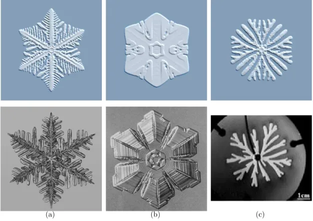
Figure 1.2: Snowflake Photographs: From left to right, the snowflake shapes transi-tion from sectored plate growth to dendritic growth. Photographs are from the Wilson “Snowflake” Bentley collection. (Bentley, 1902)

Figure 1.3: Combination of Plate and Dendritic Growth: This snowflake began growing in conditions that favored sectored plate growth, but at some point drifted into atmospheric conditions amenable to dendritic growth. This photograph is from the Wilson “Snowflake” Bentley collection. (Bentley, 1902)

of crystal structures.

In the case of frost, the defining geometric feature is dendritic growth around the boundaries, as can be seen in Figure 1.4. Far from the boundary, the ice forms a continuous plate, so visually speaking, frost can be thought of as many snowflakes that have grown together. The actual physical processes differ significantly, but a more thorough description of these differences will be left to Chapter 4. Optically, both snowflakes and frost are characteristically translucent, and in the neighborhood of sharp features, sparkling specularities tend to appear.

(25)

Figure 1.4: Photograph of frost: The main visual geometric feature is the dendritic growth along the boundary, while the main optical feature is the translucency and the sparkling specularities. The photo is from iStockPhoto.com.

• Growth that can vary continuously between the dendritic and sectored plate regimes,

• Automatic merging of nearby features that grow together,

• Optical translucency, with specularities in sharp regions.

Icicle growth poses challenges distinct from those in frost and snowflake growth. While similar physical processes are involved, this does not necessarily translate to similar computational methods. An icicle can be viewed as one large dendrite, and the rippling on the sides of an icicle can be viewed as dendrites that failed to grow due to a lack of water supply. A striking example of icicle growth can be seen in Figure 1.5.

(26)

sur-Figure 1.5: Icicles On a Fountain: Photo is from BigFoto.com.

face (Ueno, 2003; Ueno, 2004), the author of these articles admits that the thermody-namics of thin film flows still has many open questions, making analysis and taxonomy construction difficult. However, the major visual features of icicles can be conjectured from photos such as Figure 1.5. The first, most high-level observation is that icicles are conical structures that are much longer than they are thick. Second, when two icicles grow near to each other, their roots merge. Lastly, the small scale rippling on the surface of icicles cause large scale optical effects, such as rippled specularities and distorted refractions.

Explicitly, the dominant visual features of icicles are:

• Conical geometry that is much longer than it is wide,

• Automatic merging of nearby icicle roots,

(27)

1.2 The Stefan Problem

All of the previously listed visual characteristics can be understood in terms of the Stefan problem. The Stefan problem was formulated in 1889 by Josef Stefan (Stefan, 1889), who is perhaps best known for the Stefan-Boltzmann law, which relates the energy radiated by a blackbody emitter to its temperature. As a prominent scientific mind at the time when the laws of thermodynamics were first becoming well understood, Stefan was in a prime position to start addressing solidification problems.

Stefan posed his problem in the context of ocean ice forming in arctic regions, but the problem has come to represent phase transition problems in general, and has found applications in fields ranging from geology to metallurgy. The richly non-linear behavior of the problem has also attracted considerable interest in mathematics (Hill, 1987; Meirmanov, 1992). An excellent historical overview of the problem is available in (Wettlaufer, 2001). While the visual characteristics just listed can be captured in the context of Stefan problems, they each require a different version of the problem, which in turn requires different computational approaches. As the Stefan problem is the theoretical thread that unifies all of these approaches, I will now provide a high level description of the problem and describe the various versions and approximations that will later be employed.

The Stefan problem is composed of two simple equations. Assume we have a heat fieldT defined continuously over some computational domain, and an initial ice/water interface Γ. The heat field evolves according to the heat equation

∂T

∂t =D∇

2_T, _(1.1)

wheret denotes time andDdenotes a diffusion constant. The symbol∇2 _{is the}

Lapla-cian operator, which expands to ∂2

∂x2+ ∂ 2

∂y2 in 2D and ∂ 2

∂x2+ ∂ 2

∂y2+ ∂ 2

∂z2 in 3D. The ice/water interface then evolves in the normal direction according to

∂Γ

∂t ·n=D ∂T

(28)

where n denotes the normal direction. Fluid velocity and the coefficient of expansion of ice are assumed to be negligible. Stefan stated the 1D version of this problem, essentially approximating the ocean as a column of water. In 1D, the equations reduce to:

dT dt =D

d2_T

dx2 (1.3)

dΓ dt =D

dT

dx, (1.4)

where x is the spatial coordinate. The location of the ice front Γ is then obtained by integrating Eqns. 5.1 and 1.2. There are only a handful of known closed form solutions, and these only apply to simple geometries. Stefan originally solved the planar case, and subsequently the case of a sphere (Frank, 1949) and a parabola (Ivantsov, 1947) were derived. These cases are often referred to eponymously as the “Frank sphere” and “Ivantsov parabola” solutions. In the absence of a general analytical solution, solutions are usually obtained numerically. Depending on the approximations used and the boundary conditions assigned, various flavors of the Stefan problem can be obtained. In this dissertation, I will deal with the following variants: one and two sided, quasi-steady state, zero surface tension, and surface tension anisotropy.

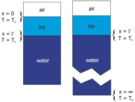
1.2.1 One and Two Sided Stefan Problems

(29)

Figure 1.6: Boundary conditions of one-sided Stefan problem: x denotes the spatial coordinate,T is the temperature, Γ is the current position of the advancing ice front, Tf is the freezing temperature of water, and Tu is some temperature less than

Tf. In the left figure, the interface evolves according to the temperature gradient in

the ice; on the right, it evolves according to the gradient in the water.

be at freezing temperature. But, unlike the case in Figure 1.6, the interface evolves according to the temperature gradient in the water, not the ice. This version allows us to define the water temperature at some far away location, usually infinity.

A two sided Stefan problem tracks heat diffusion in both the ice and the water. This case can be more difficult to simulate because the diffusion constants of water and ice differ, and handling this discontinuity at the interface can require additional considerations. I will describe methods of simulating the two-sided Stefan problem in Chapter 3 and the one-sided problem in Chapters 4 and 5.

1.2.2 The Quasi-Steady State Approximation

Stefan observed that if the diffusion constant D is very large relative to the interface velocity ∂Γ

(30)

is known as the quasi-steady state approximation, an approximation commonly used in thermodynamics to distinguish between a reversible and irreversible transformation. Eqn. 5.1 then reduces to the Laplace equation:

∇2_T _{= 0}_. _(1.5)

This greatly simplifies integration of the Stefan problem, since the entire subfield of harmonic analysis is devoted to examining the Laplace equation, and we can now draw upon this knowledge. The quasi-steady state approximation will be employed in Chapters 4 and 5.

1.2.3 Surface Tension

Surface tension is perhaps most familiar as the force that causes bubbles to form, and allows insects to walk across water surfaces. Both of these cases are examples of surface tension at a liquid/gas interface. In a more general sense, surface tension is a force that exists along any interface, including the solid/liquid interface of ice and water. Surface tension can be incorporated into the Stefan problem by adding an additional function s(θ) to Eqn. 1.2:

∂Γ

∂t ·n =D ∂T

∂ns(θ). (1.6)

The details of this function s(θ) and its role in ice pattern formation will be discussed in Chapter 3.

1.2.4 Thin Film Boundary Conditions

(31)

coats the outside of the ice. This ‘thin-film’ variant of the Stefan presents a different set of challenges, and I will describe them in detail in Chapter 5.

1.3 Thesis Statement

My thesis statement is as follows:

The visual features of ice formations such as frost, snowflakes, and icicles

can be simulated efficiently by solving appropriate versions of the Stefan

Problem.

In support of this thesis, I have constructed three different prototype systems. In the first, I use phase fields, a numerical technique from computational physics. Phase field methods correspond to the two-sided Stefan problem with surface tension anisotropy. This technique captures the first two visual characteristics of frost and snowflakes: the continuum of growth regimes between dendritic and sectored plate, and automatic merging of intersecting features. In order to address the third characteristics, the optical features of ice, I employ the photon mapping global illumination algorithm (Jensen, 2001).

Phase fields are an Eulerian simulation technique that represents the ice/water interface as an implicit surface, so the results can suffer from smoothing artifacts. In order to address this limitation, I have constructed a second system that combines phase fields with a fractal growth technique known as diffusion limited aggregation (DLA). DLA corresponds to the zero-surface tension, quasi-steady stateStefan problem. DLA is a discrete, Lagrangian simulation technique that does not suffer from smoothing artifacts. On the contrary, it can often produce features that are unnaturally sharp. By combining DLA and phase fields, I strike a middle ground between the advantages and limitations of both techniques.

(32)

quasi-steady state Stefan problem, and the literature on this particular type of Stefan problem is relatively sparse. There is no established technique akin to phase fields in the crystal growth literature, so I instead derive the necessary velocity equations for a level set simulation. The level set solver addresses the first two visual characteristics of icicles: structures that are longer than they are thick, and merging features. The last feature, optical effects due to rippling, are addressed by tracking arrival times along the surface of the icicle. A displacement shader uses these arrival times at render time to generate ripples using an analytical model from physics.

1.4 Main Results

Beyond capturing the major visual characteristics of a phenomena, there are other considerations that should be taken into account when constructing a visual simulation method. For example, it should include intuitive user parameters that can be used to drive the simulation towards a desired effect, it should be computationally efficient, and, if possible, it should be easy to implement. With this in mind, the following are the main results of this dissertation.

Chapters 3 and 4 present a method of simulating frost and snowflake formation. The main results of these two chapters are:

• A fast, simplified formulation of the phase field method for two-sided Stefan problems with surface tension anisotropy,

• Hybridization of phase fields with diffusion limited aggregation for improve cap-turing of small scale detail,

• Simple and natural aesthetic control parameters for generating desired visual effects,

(33)

• A novel discrete-continuous method that combines diffusion limited aggregation and phase field methods with a stable fluid solver,

• Accelerated and simplified computations for interactive simulation of modest-scale ice crystal growth, including a mapping to GPUs.

Chapter 5 presents a method of simulating icicle growth. The main results of this chapter are:

• A level set approach to the thin-film Stefan problem,

• An analytical solution for the tip of an icicle that appears to be in agreement with experimental data,

• A non-linear, curvature-driven evolution equation for the ice front far from the icicle tip,

• A method for simulating surface ripples the avoids the need to track small scale geometry in the simulation,

• A unified simulation framework for modeling complex ice dynamics.

1.5 Organization

(34)

(35)

Related Work

The study of pattern formation in solidification spans many different fields, including math, physics, material science, geology, and computer science. The body of literature is considerable, with entire journals (e.g. The Journal of Crystal Growth) devoted to the topic. In this section, I will give a brief a historical perspective, and then survey the works that are relevant to this dissertation.

2.1 Early Work

As mentioned in the introduction, the study of patterns in ice can be traced back to at least the 17th century with Kepler and Descartes. However, it was not until the end of the 19th century, when thermodynamics were better understood, that Stefan formulated a more quantitative model.

(36)

Figure 2.1: von Koch Snowflake: Helge von Koch defined production rules that generate structures that are qualitatively similar to those of a snowflake. While von Koch’s model is fairly simple, its easily calculated fractal dimension provides an avenue for analyzing more complex models.

Fractal geometry refers to structures that havefractional dimension. The canonical work on the subject is The Fractal Geometry of Nature (Mandelbrot, 1982). While we are accustomed to objects that have integral dimension such as 1D, 2D, and 3D, Benoit Mandelbrot famously described methods of defining in between dimensions such as 1.71D and 2.55D. The von Koch snowflake, for example, has a fractal dimension of

log 4

log 3 ≈1.26.

(37)

2.2 Related Work In Physics

Wilson “Snowflake” Bentley, a Vermont farmer with no formal scientific training, de-veloped a technique in 1885 for photographing snowflakes and constructed an extensive catalog of over 5000 snowflake images. Some of these photographs were later com-piled and published as a book (Bentley and Humphreys, 1962). Purportedly inspired by Bentley’s photographs, Japanese physicist Ukichiro Nakaya developed a method of growing snowflakes in a laboratory, and published an extensive study of crystal shapes entitled Snow Crystals, Natural and Artificial (Nakaya, 1954). In his book, Nakaya described a crystal taxonomy and the relationship between crystal shape and atmo-spheric conditions. Nakaya’s work also gave rise to additional questions, such as why the transition between different growth regimes was so abrupt.

2.2.1 Phase Field Methods

Addressing solidification problems is difficult for several reasons. The complexity of crystal structures make them resistent to analytical methods because even the selection of an appropriate coordinate system becomes difficult. The Stefan problem involves a free boundary, which means that the equations must be integrated in terms of a boundary condition that is also one of the unknowns. Finally, there is a jump in physical values at the ice/water interface, and representing this discontinuity is challenging.

(38)

each other, and the string literally becomes tangled. There are various mathematical methods for untangling or ‘de-looping’ of the results, but they are both inelegant and extremely difficult to implement.

The phase field method was first suggested by Langer (Langer, 1986) as a model of solidification. It is an implicit simulation method that does not explicitly track the location of the ice/water interface. Instead, it addressed the issue of the infinitely sharp ice/water discontinuity by smearing the interface out into a region of fast but finite transition that is resolvable on a regular grid. Langer based his work on earlier work by Halperin et al. (Halperin et al., 1974) and used the term ‘phase field’ that was coined by Fix (Fix, 1983).

Phase fields were first used to successfully simulate crystal growth of varying mor-phology by Kobayashi (Kobayashi, 1993), and since then have become the preferred simulation method in crystal growth. The simulations can be very computationally expensive however, so various techniques have been applied to the problem. Adaptive mesh refinement techniques (Provatas et al., 1999) have been used to increase the res-olution of the sres-olution around regions of interest. Additionally diffusion Monte Carlo techniques (Plapp and Karma, 2000) have been used to track the heat field far from the interface, resulting in significant computational savings. Far from the interface, heat is tracked as a set of particles whose dynamics are much cheaper to compute than flow over a mesh.

The phase field method is not directly derived from the Stefan problem, but instead follows from a free energy derivation that appeals more directly to thermodynamics. As the phase field method composes a significant portion of this dissertation, I will provide an overview of the derivation here.

(39)

choices made by Kobayashi (Kobayashi, 1993), since it is his formulation that is used in this dissertation.

The free energy F over some volume V of ice and water can be written as:

F =

Z

V

µ

f(T, p) + ε2 2|∇p|

2

¶

dV. (2.1)

The variable p is the phase variable, where p= 0 denotes water and p= 1 denotes ice, f is the energy density, and ε is a gradient entropy coefficient. Intuitively, the integral sums the energy densityf over the entire volume, but gives special treatment to regions that contain non-zero phase gradients. By definition, these regions correspond to the ice/water interface. An equation for the evolution of the phase variable p can then be obtained by taking the variational derivative ofF and applying the relation:

τ∂p ∂t =−

δF

δp. (2.2)

This relation yields:

τ∂p

∂t =∇ ·(Φ∇p) + ∂f

∂p. (2.3)

In 1D, Φ =ε2_{, and in 2D the symbol expands to the diffusion tensor:}

Φ =



 ε2 −ε∂ε∂θ

ε∂ε ∂θ ε2



_. _(2.4)

There are several possibilities for the function f, but Kobayashi uses the function

f(T, p) = p

4 4 − µ 1 2− m 3 ¶

p3₊

µ 1 4− m 2 ¶

p2_. _(2.5)

Inserting this function into Eqn. 2.6, we obtain the final evolution equation for p:

τ∂p

∂t =∇ ·(Φ∇p) +p(1−p)

µ

p−1 2 +m

¶

. (2.6)

For the symbol m, Kobayashi selects the function m(T) = α

(40)

whereα,π, andγ are constants, and Teis the freezing temperature of water. Explicitly

multiplying through the diffusion tensor gives the 2D evolution equation:

τ∂p

∂t =∇ ·(ε

2_∇_p₎₋ ∂

∂x

µ

εε0∂p ∂y

¶

+ ∂ ∂y

µ

εε0∂p ∂x

¶

+p(1−p)

µ

p− 1 2 +m

¶

. (2.7)

Subsequent work has rigorously proved that in the limit, limε→0τ∂p_∂t, the phase field

equations do indeed converge to the Stefan problem with surface tension (Caginalp and Chen, 1992).

2.2.2 Level Set Methods

Level set methods, an alternate implicit front tracking strategy, has also been success-ful in simulating crystal formation. Level set methods were first developed by Osher and Sethian (Osher and Sethian, 1988) as a general front tracking strategy, and have since found numerous applications including computational fluid dynamics (Foster and Metaxas, 1996), lithography (Adalsteinsson and Sethian, 1995b; Adalsteinsson and Sethian, 1995c; Adalsteinsson and Sethian, 1997), and computer vision (Malladi et al., 1995). Both Osher (Osher and Fedkiw, 2003) and Sethian (Sethian, 1999) have written books that exhaustively describe level set methods, the wide variety of techniques that have been developed surrounding them, and their numerous applications.

Whereas phase fields smear out the location of the ice/water interface, level set methods track the precise position of this interface. Instead of tracking a phase order parameter p, the level set method tracks the evolution of some implicit function φ, usually a signed distance function. Whereas the phase field method essentially relies on a reaction equation to correctly evolve the interface, level set methods construct a velocity field vover the entire computational domain and then evolve φ according to

∂φ

(41)

The nomenclature of phase field and level set methods can unfortunately overlap, because in a general sense ‘level sets’ refer to the isosurface of an implicit function. Therefore the interface location in phase fields is sometimes referred to as the ‘0.5 level set’ or the ‘zero level set’, depending on if thepparameter is defined over [0,1] or [-1,1]. To avoid confusion, I will only use the term ‘level set’ in this dissertation when referring to the level set method.

Since phase fields only converge to the Stefan problem in the limit, it has been argued that they are only a first order accurate tracking method (Gibou et al., 2003). Level set methods were first applied to the problem of solidification in by Sethian and Strain (Sethian and Strain, 1992) using a boundary integral approach. A simpler method was later suggested by Chen et. al. (Chen et al., 1997) and later extended in a pair of articles (Gibou et al., 2003; Gibou and Fedkiw, 2005) to second and fourth order accuracy.

The strategy followed level set simulation of the Stefan problem is slightly different from that of the phase field method. While both use an implicit function to track the interface, the level set approach essentially constructs a temporary explicit represen-tation every timestep. Since the implicit function used is a signed distance function instead of a phase order parameter, it is possible to locate the explicit interface with much higher accuracy than in phase field methods. Once this is done, the boundary is set according to the the Gibbs-Thomson relation,

TI =εcκ−εvVn

whereTI is the temperature at the interface, εc is a surface tension coefficient,κ is the

local curvature,εv is the molecular kinetic coefficient, and Vn is the normal velocity of

the interface.

(42)

set simulator require a velocity to be defined over the entire computational domain. This problem is overcome by interpolating the computed interface velocities back into their corresponding grid cells, and then extending the values over the entire simulation domain using an extension velocities method (Adalsteinsson and Sethian, 1999).

While the level set approach does yield higher numerical accuracy, it utilizes a good deal more numerical machinery than the phase field method. For simplicity, I use the phase field method in chapters 3 and 4. However, for the case of icicle growth, some of the features of level set methods become necessary, so I use them in chapter 5.

2.2.3 Thin Film Growth

All of the above work deals with growth in the presence of a large water supply. The previous work in phase fields and level set methods assume that the crystal is growing in an infinite bath of supercooled water, and Nakaya’s snowflake work assumes that a large supply of water vapor is present in the atmosphere. Icicle growth instead deals with the case where the water supply is severely limited.

In glaciology, there exists some work on the problem of thin-film ice growth. Several analytical models exist for icicle formation (Maeno et al., 1994; Makkonen, 1988; Szilder and Lozowski, 1994), but these models are concerned with accurately capturing the ratio of an icicle’s length to its radius. These models are derived using an energy balance approach using a plethora of environmental variables that are of limited value to the simulations addressed in this dissertation. For example, the Makkonen model (Makkonen, 1988) is composed of the two equations

−hta+h

0.622Le

cppa

(e(0o_C₎₋_Re₍_t

a))−σ×ata=

3.74cw

d2

·

W0−πLD

·

ρa1

2 dD

dt +h 0.622

cppa

(e(0o)C−Re(ta)))

¸¸ × · dL dt − 1 2 dD dt

¸₀_.₅₈₈

+ 2Lfρiδ(d−δ) d2

(43)

symbol definition

h convective heat-transfer coefficient ta air temperature

Le latent heat of evaporation

cp specific heat of water

pa air pressure

e(0o_C₎ _{saturation water-vapor pressure}

R Relative humidity

e(ta) saturation water-vapor pressure

σ Stefan-Boltzmann constant d diameter of pendant drop W0 mass flux of water to tip

ρa density of icicle walls

ρi ice density

δ wall thickness at tip

Table 2.1: Symbols for the Makkonen (Makkonen, 1988) model.

and

dD dt =

−hwta+hw0.622_c_p_p_aLe [e(0o)C−Re(ta)]−σata

1

2ρaLf(1−λ)

.

The symbols are summarized in Table 2.1. The model involves pressures and den-sities that ideally would be abstracted away in a visual simulation model. To this end, I will forgo the glaciology models and instead derive a novel equation for icicle tip dy-namics in Chapter 5. The analytical models from glaciology are not directly applicable to visual simulation, as they would merely generate simple cones and cannot capture surface rippling effects. Thin film ice formation is also a topic of interest in mechanical engineering, as ice forming on the wing of an aircraft is a hazardous scenario. The Messinger model (Messinger, 1953) is the standard method of determining when ice will form, and is an energy balance model that is also not directly applicable to visual simulation. Myers and Hammond (Myers and Hammond, 1999) recast the problem as a thin film Stefan problem, but only solve the 1D case.

(44)

understood phenomena. However, Ogawa and Furukawa (Ogawa and Furukawa, 2002) recently proposed a model of ripple formation which was subsequently refined by Ueno in a pair of articles (Ueno, 2003; Ueno, 2004). The former model only applies to a cylinder, and the latter model was derived for an inclined plane. Ueno’s model will later be used in Chapter 5 to simulate ripple formation along the surface of an icicle.

2.2.4 Laplacian Growth

Laplacian growth is a general class of physical phenomena that includes ice growth, lightning formation, liquid surface tension, quasi-steady state fracture, and river for-mation, among others. The unifying notion is that patterns form according to a field that satisfies the Laplace equation (Eqn. 1.5). In the case of ice formation, this field corresponds to a quasi-steady state heat field. In other phenomena, the correspondence differs. In lightning and surface tension for example, the field corresponds to electric potential and fluid pressure.

A Laplacian growth simulation technique that has received a good deal of attention in the physics literature is diffusion limited aggregation, usually abbreviated as DLA (Witten and Sander, 1981). Originally formulated as a model of aggregating metal particles, it has since found success in various other phenomena, including snowflake growth (Family et al., 1987; Nittmann and Stanley, 1987). One of the defining charac-teristics of DLA is that it produces fractal structures. In 2D, DLA produces structures of approximatelyD≈1.71, and in 3D, D≈2.55.

(45)

At first glance, it is not obvious that DLA corresponds to a Stefan problem, as it does not involve any differential equations. However, there are several algorithms that generate results that are visually indistinguishable from the results of DLA. One of these algorithms, thedielectric breakdown model(DBM) (Niemeyer et al., 1984) utilizes the Laplace equation (Eqn. 1.5) where DLA uses a random walk. I will later use DBM in Chapter 4 to describe the relationship of DLA to a Stefan problem.

2.3 Analytical Solutions to the Stefan Problem

There are a handful of known analytical solutions to the Stefan problem, and they only apply over simple geometries. However, I will use these solutions and their derivations later in chapter 5 to derive thin-film equivalents, so I will describe the classical ‘infinite water’ derivations here.

2.3.1 Planar Case

The planar case of the Stefan problem involves one coordinate, usually denoted as the negative z direction. This is because Stefan originally formulated the problem in terms of ocean ice forming, and the ice forms first at the surface of the water and gradually thickens downwards into an infinitely deep ocean. There are several different approaches to solving the 1D equations, but I will use the ‘moving-frame’ approach described in Saito (Saito, 1996). In this case we assume that the global coordinate is z, but introduce a moving variable z0 ₌_z₋_{V t}_{, where} _V _{is velocity and} _t _{is time. In} this way, at any time t, z0 _{= 0 denotes the current location of the interface. In terms} of this moving frame, the diffusion equation becomes

1 D

∂T ∂t =∇

2_T ₊ 2

lD

∂T ∂z0

where D is again the thermal diffusion constant and lD = 2_VD. Applying the

(46)

∇2_T ₊ 2

lD

∂T ∂z0 = 0.

By specifying an infinitely far away boundary condition T(z0 ₌ _{∞) = 0, this can} be integrated to

T(z0_{) =}_Ae−2z_lD0_,

whereAis an as yet undetermined constant of integration. The second equation in the 1D Stefan problem can now be written as:

dz0

dt =−D dT

dz.

In this form, it can be solved by plugging in the T(z0_{) to obtain:}

dz0

dt =−D 2A

lD

=AV.

Since V = dz0

dt, this means that the constant A must be equal to 1. We then apply

the Wilson-Frenkel law:

dz0

dt =K((Tu)−Ti−dκ),

where K is the kinetic coefficient, Tu is the undercooling of the water, Ti is the

tem-perature at the interface, d is the capillary length, and κ is the curvature. Applying this to the velocity equation, we obtain the final velocity of the planar interface:

dz0

dt =K(Tu−1).

(47)

2.3.2 Spherical Case

The case of a sphere was solved by Frank (Frank, 1949), and is thus sometimes referred to as the ‘Frank sphere’ case. Again, I follow the derivation given by Saito (Saito, 1996). The case is again 1D, but instead of the cartesian coordinate z, we have the radial coordinater, and the moving frame isr0 _{instead of} _z0_{. The diffusion equation in} spherical coordinates is:

1 D ∂T ∂t = µ ∂2

∂r2 +

2 r ∂ ∂r ¶ T.

Again applying the quasi-steady state approximation, we obtain:

µ

∂2

∂r2 +

2 r

∂ ∂r

¶

T = 0.

Similar to the planar case, we specify an infinitely far away boundary condition T(r0 ₌_{∞) = 0, and obtain the solution}_T₍_r_{) =} A

r. Ais again an undetermined constant

of integration. Applying the second equation of the Stefan problem, we obtain:

dr0 dt =

DA (r0₎2.

Again applying the Wilson-Frenkel law, we obtain:

dr0 dt =K

µ

Tu−

A r0 −

2d r0

¶

.

Using these two equations, the constant of integrationA is uniquely determined as:

A= (r 0₎2¡_T

u−2_rd0

¢

r0₊ D K

.

The final velocity equation is then:

dr0 dt =

D¡Tu −2_rd0

¢

r0₊ D K

.

The detail to note is that below a certain radius, 2d

(48)

the planar case, when the sphere does grow, it does not have a constant velocity, and instead the velocity slows as the radius increases.

2.3.3 Parabolic Case

In the parabolic case, we assume that the growing crystal takes the form of a parabola, and obtain an expression for the velocity of the tip. The original solution was obtained by Ivantsov (Ivantsov, 1947), but again I follow the derivation in Saito (Saito, 1996). To characterize the position of the tip, we use the same z and z0 _{coordinates from the} planar case, but in this case z0 _{denotes the location of a parabola tip, not a plane. We} then define a parabolic coordinate system around the z axis:

ξ = r−z0

η = r+z0

θ = arctan(x/y).

In this case, r is defined as r = px2₊_y2_{+ (}_z0₎2_{. The parabolic version of the}

quasi-steady state heat equation can be written as:

1 η+ξ

µ ∂ ∂ηη ∂T ∂η + ∂ ∂ξξ ∂T ∂ξ ¶ + 1 4ηξ

∂2_T

∂θ2 +

1 lD

1 η+ξ

µ

η∂T ∂η −ξ

∂T ∂ξ

¶

= 0.

If we assume circular symmetry, this reduces to:

∂ ∂η µ η∂T ∂η ¶ + 1 lD µ η∂T ∂η ¶

= 0.

Denoting the current location of the interface as ηi, the second equation of the

Stefan problem translates to:

ηi +ξ

∂ηi

∂ξ + ηi+ξ

2V ∂ηi

∂t =−lD

µ

ηi

∂u ∂η −ξ

∂ηi

∂ξ ∂T

∂ξ − ηi+ξ

4ηiξ

(49)

Using the boundary condition T(ηi) = Tu, the temperature field integrates to:

T(η) = Tu+C

Z _η

R

e−lDx x dx.

The symbol R denotes the radius of curvature of the parabola tip and C is a constant of integration. Using the boundary conditionT(η=∞) = 0, we can solve for the value of C,

C =−_R Tu ∞ R e −x lD x dx ,

and obtain the heat solution:

T(η) = Tu

 ₁₋

R_η R e −x lD x dx R_∞ R e− x lD x dx  _.

Inserting this heat solution into the second equation of the Stefan problem, we obtain what is known as the ‘Ivantsov relation’:

Tu =

R lD

elDR

Z _∞

R

e−lDx x .

The relation is usually simplified using the change of variables P = R

lD and expo-nential notation E1(P) =

R_∞

P e

−x

x to obtain:

Tu =P ePE1(P). (2.8)

For small undercoolings, this relation is sometimes approximated in 3D as Tu ≈

P(−logP −γ), where γ is the Euler-Mascheroni constant, and in 2D as Tu ≈

√ πP. The feature to note is that the Ivantsov relation is that given an undercoooling Tu, it can only be solved for the product of the radius of curvature and the velocity,

(50)

A good deal of effort has been devoted to determining the nature of this additional constraint. ‘Microscopic solvability theory’ (see for example (Brener and Mel‘nikov, 1991)) suggests that the missing constraint is surface tension. Fortunately, in the case of icicle growth, experimental measurements show that the radius of the icicle tip stays relatively stationary under a wide variety of undercoolings, so in the case of this dissertation, an appeal to microscopic solvability theory is unnecessary.

2.3.4 Cylindrical Case

The cylindrical case corresponds to the case where a small column of undercooled water is surrounded by ice. I will follow the derivation given by Hill (Hill, 1987) here. The heat equation in cylindrical coordinates is:

∂T ∂t =D

µ

∂2_T

∂r2 +

1 r ∂T ∂r + 1 r2

∂2_T

∂θ2 +

∂2_T

∂y2

¶

.

Applying the quasi-steady state approximation and assuming homogeneity in all but the radial direction, this reduces to:

∂2_T

∂r2 +

1 r

∂T ∂r = 0.

The solution must be of the form

T(r, t) =A+Blogr.

As before, the interfacer0 _{is constrained to the freezing temperature}_T

f, but instead

of applying the Wilson-Frenkel law at the interface, we apply Newton cooling:

T(1, t) +β∂T(1, r) ∂r = 1.

(51)

A+Blog 1 +βB

1 = A+βB = 1 A+Blogr0 ₌ _T

f.

We can then solve for A and B:

A = −(1−Tf) logr0 β−logr0

B = 1−Tf β−logr0

Thus the heat field solves to:

T(r, t) = logr−(1−Tf) logr0 β−logr0

Inserting this into the second equation of the Stefan problem yields:

dr0

dt =−D ∂T ∂r0 =

−D r0₍_β₋_log_r0₎.

This equation can be integrated if first inverted,

dt dr0 =

−r0₍_β₋_log_r0₎

D ,

and then integrated with respect to r0 _{to get an ‘arrival time’ equation:}

t(r0_{) =} 1 4D(2(r

0₎2_log_r0₋_{(1 + 2}_β₎₍₁₋₍_r0₎2₎₎_.

The identity R xlogx dx= x2

2(logx− 12) was applied in order to perform this

inte-gration. Intuitively, this equation describes the time at which the interface will arrive at some radiusr0_{. Instead of performing this final integration, I will later use a thin-film} variant of the dr0

(52)

2.4 Related Work In Graphics

2.4.1 Phase Transition

Phase transition is a relatively new topic in computer graphics, because until recently, robust, efficient solvers for objects of a single state were not commonly available. Clearly, it would be difficult to simulate an object transitioning from solid to liquid in the absence of robust rigid body and fluid simulators.

In particular, recent techniques used for fluid simulation are relevant to this disser-tation, since I use many of the same techniques to track the rapidly evolving ice surface. Early work in fluid simulation solved the Navier-Stokes equations using the Marker-In-Cell (MAC) method (Foster and Metaxas, 1996) from computational fluid dynamics (Harlow and Welch, 1966), and also efficiently solved the shallow water equations (Kass and Miller, 1990).

In his seminal 1999 paper, Stam described a fast, unconditionally stable method of simulating the Navier-Stokes equations (Stam, 1999b). Subsequently, considerable re-search effort has been devoted to building on Stam’s ideas and formulating alternative approaches. Free boundaries were added to take into account pouring and splashing (Enright et al., 2002b; Foster and Fedkiw, 2001), and the concept of ‘vorticity con-finement’ was introduced to counteract numerical smearing (Fedkiw et al., 2001). An efficient method of simulating smoke and water on an octree data structure was also introduced (Losasso et al., 2004). I will later use similar techniques for icicle simulation.

(53)

forcing terms involved in melting simulations, and Losasso et al. (Losasso et al., 2005) described a method of melting Lagrangian solids into Eulerian liquids.

Other work has also dealt with visco-elastic objects that possess viscosities much higher than water, but still exhibit flowing behavior (Goktekin et al., 2004; Clavet et al., 2005). These works do not appear to handle large viscosity transitions however, so the methods are not directly applicable to solidification.

2.4.2 Modeling Winter Scenes

The problem of modeling a winter scene has received attention in graphics because it gives rise to a unique set of challenges. Fallen snow has a specific geometric shape that cannot be captured by simply offsetting existing scene geometry. More sophisticated, physically-based approaches have been attempted such as the use of metaballs (Nishita et al., 1997), and a ‘visible sky’ algorithm (Fearing, 2000) that is similar to the ambient occlusion algorithm in global illumination. Recent work has also successfully modeled the appearance of snow falling from the sky (Langer et al., 2004).

Modeling ice formation in these scenes has not been as closely examined. To my knowledge, the only work that bears some resemblance to that presented here is by Kharitonsky and Gonczarowski (Kharitonsky and Gonczarowski, 1993). They de-scribed a random-walk model of icicle growth, where water droplets walk along an ice surface and freeze with a certain probability. However, their approach does not naturally handle the formation of more than one icicle. More seriously, the notion that icicles form as the aggregate of discrete droplets is not empirically supported.

2.4.3 Pattern Formation

(54)

(Bodenschatz et al., 2003). In this sense, the work in this dissertation is one of many pattern formation algorithms in computer graphics. The patterns that form in fluid simulation, for example, fall into this category due to the non-linear advection term. Visual phenomena that arise as a consequence of flow, such as sand dunes and rust patterns (Dorsey et al., 1996; Chen et al., 2005) meet this criteria as well.

Closely related to the phase field equations to be presented in Chapter 3 are reaction-diffusion systems. Pattern formation in reaction-reaction-diffusion systems was first described by Turing (Turing, 1952). The notion is counter-intuitive, because diffusion is usually thought of as a physical mechanism that smears out detail, not one that gives rise to it. However, Turing showed that when coupled with the appropriate reaction terms, sharp, standing wave solutions could be obtained. The formation mechanism has since been dubbed ‘Turing instability’ in physics. Reaction-diffusion was introduced to graphics by two articles that were published concurrently: (Witkin and Kass, 1991) and (Turk, 1991). The first article (Witkin and Kass, 1991) described how to simulate reaction-diffusion over a rectilinear grid. However, when this grid is stretched over a model, it experiences significant distortion, so a distortion correction technique was described as well. The second article (Turk, 1991) circumvented the distortion problem by generat-ing a Voronoi diagram on the surface of the model in lieu of a rectilinear grid and then solved the reaction-diffusion equations over the diagram instead. Reaction-diffusion equations have the form:

∂A

∂t =DA∇

2_A₊_R₍_A₎_.

The symbol A denotes some chemical, DA is its diffusion constant, and R(A) is

(55)

∂A

∂t = DA∇

2_A₊_R₍_{A, B}₎

∂B

∂t = DB∇

2_B ₊_R₍_{A, B}₎_.

In fact, the phase field equations can be viewed as a special case of reaction diffusion. In both cases, non-trivial patterns form from initially homogeneous concentrations due to non-linearities in the reaction equations.

DLA, the algorithm that will be presented in Chapter 4 has also been applied to pattern formation in other phenomena, such as lichen growth (Sumner, 2001; Desbenoit et al., 2004). DBM, which also be described in Chapter 4 has been used to simulate lightning (Kim and Lin, 2004). In both of these cases, the non-linearity arises from the implicit presence of Eqn. 1.2 in the simulation.

(56)

(57)

The Phase Field Method

In this chapter, I describe one method of solving the Stefan problem, the phase field

method. The general approach of the phase field method was derived independent of the Stefan problem, using an approach that appeals more directly to thermodynamics. A summary of this free energy approach is available in the previous chapter. I will provide an overview of the phase field equations and describe how they intuitively map to the Stefan problem.

Additionally, I present techniques to simplify the phase field computation and make the problem of simulating ice crystal growth more tractable. I also show how the phase field method allows a user parameterization that a visual effects artist can use to manip-ulate the ice crystal growth. The phase field method often has smoothing artifacts as a result of its implicit representation, and it can only compute the outermost ice/water boundary. Therefore, a novel intermediate geometric processing step is introduced to add sharp edges and medial ridges to the interior of the ice. Finally, the simulated images are rendered using photon mapping (Jensen, 2001).

(58)

Figure 3.1: Detail of ice grown on a stained glass window. The inset shows the full window.

3.1 Overview

I will give a brief overview of the overall computational framework and the basic design of each step involved.

I use a simple and powerful implicit simulation technique from the crystal growth literature, known as the phase field method. This method can takeO(N3_{) time, where}

N is the resolution of a single grid dimension. To obtain reasonable accuracy, N must be fairly large, making the computation quite expensive. I reduce the computation time significantly by using two acceleration techniques. The first is based on the observation that most ice crystals are very thin. I can simulate growth in 2D and add 3D detail later, reducing the computation time from O(N3_{) to} _O₍_N2_{). Second, I further improve the}

performance of the simulation by performing banded computation around the “front” of the ice and water interface, instead of over the entire grid.

(59)

The visually salient features of our target object are used for the seed crystal. The features are extracted with edge detection and used to set the initial conditions of the simulation. In addition to seeding the simulation, I also influence the simulation throughout by manipulating the freezing temperature.

Due to the smoothing artifacts of the phase field method and the lack of internal detail given by the evolving interface, a novel intermediate geometric processing step is introduced to add sharp features prior to rendering. This is performed by first computing the border and medial axis of the ice with morphological operators. Given the resulting medial axis and boundary edges, I generate a constrained conforming Delaunay triangulation upon which a subdivision step is performed to introduce creases and edges (DeRose et al., 1998). Finally, the triangles are rendered using photon mapping (Jensen, 2001).

Fig. 3.2 shows the overall system pipeline of our computational framework.

Figure 3.2: The overall system pipeline.

3.2 The Phase Field Method

(60)

the major objectives of this dissertation described in Chapter 1, as they are able to simulate the range of growth regimes between dendritic and sectored plate growth.

Subsections [3.2.1] - [3.2.3] give an overview of the method, and present Kobayashi’s formulation (Kobayashi, 1993). The relationship of phase field methods to the Stefan problem are described in subsection [3.2.4]. In subsections [3.2.5] - [3.2.8] I will present my own analysis and optimizations.

3.2.1 Undercooled Solidification

An undercooled liquid is a liquid that has been cooled below its freezing temperature, but has been cooled sufficiently slowly for it to remain in its liquid state. When a small amount of solid material, known as the seed crystal, enters a container filled with undercooled liquid, the liquid transitions to solid radially outwards from the initial seed in a rapid and unstable reaction. Due to this instability, the growth of the crystal can be influenced by small perturbations, such as surface tension or minute impurities in the liquid. These factors can lead to the complex branching, or “dendritic”, behavior we see in ice.

3.2.2 The Phase Field

In the phase field method, the undercooled liquid is represented implicitly as a two or three-dimensional grid. This is also known as an ‘Eulerian’ representation. Many papers in computer graphics describe Eulerian simulation in detail (Witkin and Kass, 1991), as does any general applied linear algebra text (Demmel, 1997). For simplicity and tractability, I limit the simulations to two dimensions.

Two separate fields are tracked using this discrete representation: A temperature field T, records the amount of heat in a given cell, and a phase field p records the current phase of a given cell. For a given grid coordinate (x, y),Txy and pxy are defined

as the corresponding values in the temperature and phase fields.

(61)

cell contains ice. If pxy is between [0,1], then it is at an intermediate stage between

the two states. While phase is usually thought of as a binary state, either water or ice, on the microscopic level there is a continuum of states along the ice front. The phase field method makes the computation of solidification tractable by magnifying this microscopic continuum so that it is visible macroscopically.

(a) (b)

Figure 3.3: (a) A phase field in which white is p= 1 (ice), and black is p= 0 (water). The gray band in the middle is the section shown in profile in (b). (b) Cross section from (a) in profile. Note that while the transition from water to ice is abrupt, it is not instantaneous.

Fig. 3.3(a) is an example of a partially reacted phase field, and Fig. 3.3(b) is a cross section from Fig. 3.3(a). The horizontal axis of Fig. 3.3(b) is the spatial dimension, and the vertical axis is the phase dimension. In actuality, the transition from p= 1 (ice) to p= 0 (water) should be a microscopically thin, virtually instantaneous step function. Instead, the microscopic transition has been magnified, and we can see a region of quick but finite transition. Once the interface has been magnified to a resolution where non-integral values of pxy appear on the grid, we can evolve the interface by applying

Physically-based simulation of ice formation

ACKNOWLEDGMENTS

TABLE OF CONTENTS

LIST OF FIGURES

LIST OF TABLES

Introduction

1.1

Visual Characteristics

1.2

The Stefan Problem

1.2.1

One and Two Sided Stefan Problems

1.2.2

The Quasi-Steady State Approximation

1.2.3

Surface Tension

1.2.4

Thin Film Boundary Conditions

1.3

Thesis Statement

1.4

Main Results

1.5

Organization

Related Work

2.1

Early Work

2.2

Related Work In Physics

2.2.1

Phase Field Methods

2.2.2

Level Set Methods

2.2.3

Thin Film Growth

2.2.4

Laplacian Growth

2.3

Analytical Solutions to the Stefan Problem

2.3.1

Planar Case

2.3.2

Spherical Case

2.3.3

Parabolic Case

2.3.4

Cylindrical Case

2.4

Related Work In Graphics

2.4.1

Phase Transition

2.4.2

Modeling Winter Scenes

2.4.3

Pattern Formation

The Phase Field Method

3.1

Overview

3.2

The Phase Field Method

3.2.1

Undercooled Solidification

3.2.2

The Phase Field