GENETIC ASSOCIATION ANALYSIS ON SECONDARY PHENOTYPES AND GROUP CONDITIONAL VARIABLE IMPORTANCE IN OPPERA STUDY
Wei Xue
A dissertation submitted to the faculty at the University of North Carolina at Chapel Hill in partial fulfillment of the requirements for the degree of Doctor of Public Health in the
Department of Biostatistics in the Gillings School of Global Public Health.
Chapel Hill 2016
Approved by: Eric Bair Mengjie Chen Yun Li
c
○ 2016 Wei Xue
ABSTRACT
Wei Xue: Genetic Association Analysis on Secondary Phenotypes and Group Conditional Variable Importance in OPPERA Study
(Under the direction of Eric Bair)
Temporomandibular disorder (TMD) is a complex chronic painful orofacial disorder re-sulting in dysfunction in the temporomandibular joints and the muscles around the jaw. Numerous risk factors were studied and identified for the chronic and onset of TMD. The Orofacial Pain: Prospective Evaluation and Risk Assessment (OPPERA) study is a prospec-tive study designed to study the etiology and the risk factors contributing to the onset and chronic TMD (Smith et al. 2011).
Genetic risk factors play an important role in the etiology of TMD. While many stud-ies identified the genetic variants associated with TMD case-control status, one may wish to identify genetic markers associated with secondary phenotypes (such as clinical pain) that are related to the severity of TMD. In such cases, naive regression methods that ig-nore the case-control design produces biased results. This problem may be corrected by statistical methods such as inverse probability weighting (IPW). However, it may be unre-liable when genetic markers and secondary phenotypes are strongly associated with case-control status. In order to perform unbiased association analysis, we proposed a novel permutation-based IPW method, and compared it with conventional IPW method. The results indicated that the permutation-based IPW produced controlled type I error rates with no loss in power. The application to the data from OPPERA study identified the as-sociated SNPs with the severity of orofacial pain.
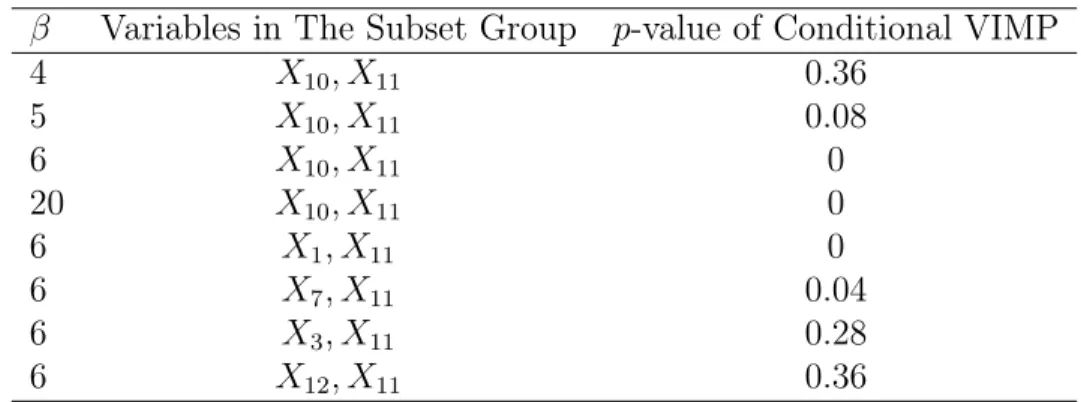
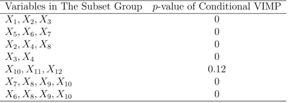
high variable important (VIMP) score conditional on existing risk factors. The are curious to know that in addition to the existing variables, would the group variables bring more information in predicting outcome. For example, they want to know if the group impor-tance score for measuring mechanical and thermal pain sensitivity is significantly different from 0 conditional on all the other variables when predicting either chronic or first-onset TMD.
In the second project, we proposed a method to test the group conditional variable im-portance statistically, by conditional distribution of group variables on the those outside the group using random forest model. Simulations were performed by continuous and cate-gorical variable types. p-values were calculated for some groups. This method corrects the shortcomings of the likelihood of choosing correlated variables with spurious correlation, and provided a way of testing group variables without bias.
To Yanping Shi and Zhixin Xue, my parents who give me unconditional love and support. To Kai Xia, my husband and my best friend.
ACKNOWLEDGMENTS
I would like to express my deepest gratitude to my DrPH advisor Dr. Eric Bair for his fully unwavering support and mentorship in my dissertation. This dissertation cannot be finished without his patience, wisdom, understanding and guidance. I would also like to express my appreciation to my committee members Dr. Donglin Zeng, Dr. Yun Li, Dr. Mengjie Chen and Dr. Shad Smith for their valued comments.
I would also like to thank my parents and my in-laws. Without their unconditional love and help to taking care of my kids and me, I cannot finish the dissertation on time.
I would like to dedicate my dissertation to my beloved kids Yo-Yo and Mo-Mo. They are the angel in my life. Their little smile shed lights on me, and give me the power to move on.
TABLE OF CONTENTS
LIST OF TABLES ... x
LIST OF FIGURES ... xi
CHAPTER 1: INTRODUCTION ... 1
CHAPTER 2: LITERATURE REVIEW ... 5
2.1 Statistical Methods and Background Information in Secondary Phenotypes and Genetic Association Studies... 5
2.1.1 Genetic Association Studies ... 5
2.1.2 The analsyis of secondary phenotype in ge-netic association studies... 7
2.1.3 Principal component analysis (PCA) ... 9
2.1.4 Permutation... 11
2.2 Random Forests and Variable Importance ... 12
2.2.1 Random Forests Model... 12
2.2.2 Variable Importance (VIMP) in Random Forest ... 13
2.2.3 Strobl’s Conditional VIMP ... 15
2.3 OPPERA study ... 16
2.3.1 Temporomandibular Disorder (TMD)... 16
2.3.2 Overview of OPPERA ... 17
2.3.3 Studies of putative risk factors and TMD ... 18
2.3.4 Genetic Associations with TMD in OPPERA ... 20
3.1 Introduction ... 21
3.2 Method ... 24
3.2.1 Permutation-based IPW ... 24
3.2.2 Type I error simulation ... 27
3.2.3 Power Simulation ... 30
3.2.4 Data Application ... 31
3.3 Results... 32
3.3.1 Type I Error ... 32
3.3.2 Statistical Power ... 34
3.3.3 Data application ... 34
3.4 Discussion ... 35
CHAPTER 4: CONDITIONAL VARIABLE IMPORTANCE TEST IN RANDOM FORESTS ... 44
4.1 Introduction ... 44
4.2 Methods ... 49
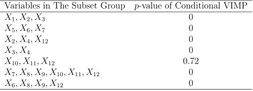
4.2.1 Conditional VIMP on a subset of variables ... 49
4.2.2 Statistical test for conditional VIMP on a sub-set of variables ... 50
4.3 Simulation Studies ... 52
4.3.1 Simulation 1, simulation of quantitative out-come and predictors ... 53
4.3.2 Simulation 2: simulation of quantitative out-come, predictors and adding interaction term ... 55
4.3.3 Simulation 3, simulation with binary outcome and quantitative variables. ... 56
4.3.4 Simulation 4, simulation with binary outcome and quantitative and qualitative variables. ... 58
CHAPTER 5: CONDITIONAL VIMP AND STATISTICAL
TEST IN OPPERA STUDY ... 65
5.1 Introduction ... 65
5.2 Methods ... 68
5.2.1 OPPERA study description ... 68
5.2.2 Study Measurenment of Risk factors in TMD ... 69
5.2.3 Statistical Analysis ... 73
5.3 Results... 76
5.3.1 Additional Measurements in First-onset TMD ... 80
5.4 Discussion ... 82
CHAPTER 6: SUMMARY AND FUTURE RESEARCH... 88
LIST OF TABLES
3.1 Power simulation... 43 4.2 Simulation Results of Conditional VIMP in Variable
Subset forSimulation 1, ... 61 4.3 Simulation Results of Conditional VIMP in Variable
Subset forSimulation 2, ... 62 4.4 Simulation Results of Conditional VIMP in Variable
Subset forSimulation 3, ... 63 4.5 Simulation Results of Conditional VIMP in Variable
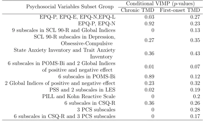
Subset forSimulation 4, ... 64 5.6 Conditional VIMPp-values in Psychosocial Risk
Fac-tors Subsets on Chronic and First-onset TMD ... 78 5.7 Conditional VIMP p-values in Autonomic Risk
Fac-tors Subsets on Chronic and First-onset TMD ... 79 5.8 Conditional VIMP p-values in Pain Sensitivity Risk
LIST OF FIGURES
3.1 QQ plot of the p-values produced by the
permutation-based IPW method for the first simulation scenario ... 38 3.2 QQ plot of the p-values produced by conventional
IPW regression for the first simulation scenario ... 39 3.3 QQ plot of the p-values produced by the
permutation-based IPW method for the second simulation scenario ... 40 3.4 QQ plot of the p-values produced by conventional
IPW regression for the second simulation scenario ... 41 3.5 QQ plot of the p-values for testing the null hypothesis
of no association between each SNP and pain density
CHAPTER 1: INTRODUCTION
Chronic pain is a significant and costly health problem . In particular, temporomandibu-lar disorder (TMD) is a complex chronic painful orofacial disorder resulting in dysfunction in the temporomandibular joints and the muscles around the jaw. It has a prevalence of around 5% in adults in US 2012 National Health Interview survey (Isong et al. 2008). Nu-merous risk factors were studied and identified for the chronic and onset of TMD, such as pain sensitivity risk factors, clinical risk factors, psychological distress, and genetic factors. The Orofacial Pain: Prospective Evaluation and Risk Assessment (OPPERA) study is a prospective study designed to study the etiology and find out the risk factors contributing to the onset and chronic TMD (Smith et al. 2011). The study patients filled out question-naires and underwent a series of clinic examinations for potential risk factors for TMD. Blood sample was drawn from each participants and genotyped for genome-wide associa-tion study (GWAS).
a case-control study (Richardson et al. 2007) and (Monsees et al. 2009). However, con-ventional IPW regression may be unreliable when evaluating the association between ge-netic markers and secondary phenotypes that are strongly associated with case status. In a TMD case-control study, one may wish to identify genetic markers associated with the severity of orofacial pain, which is present in all TMD cases, but nearly all controls report no orofacial pain, causing conventional IPW regression to produce inflated type I errors and inaccurate results. In order to perform the association analysis, we proposed a novel permutation-based IPW method in the first project, and compared it with con-ventional IPW method. The results from simulations indicated that whereas concon-ventional IPW method might produced inflated type I error rates, the permutation-based IPW pro-duced correct type I error rates with no loss in power. We then applied this method to data from OPPERA case-control study to identify the associations between candidate SNPs and the severity of orofacial pain. Two novel SNPs were identified associated with TMD pain severity by our method.
successfully avoid choosing spurious variables as important ones. Based on the methodol-ogy, people may be curious to know whether a group of variables are significantly impor-tant to the outcome (which might be chronic or first-onset TMD) conditional on the rest risk factors. Researchers in OPPERA study are especially interested in such questions be-cause of the large amount of variables and the high correlations among them in OPPERA case-control study and cohort study. For example, one may wish to know if the group im-portance score for measuring mechanical and thermal pain sensitivity is significantly dif-ferent from 0 when predicting either chronic or first-onset TMD conditional on the other existing variables.
In the second project, we proposed a method to statistically test the group conditional variable importance, by using conditional distribution of variables in the group on the those outside the group in random forest. The idea behind the scene is when the vari-ables in the group are important conditional on the other varivari-ables, they would bring more information significantly in predicting the outcome in addition to variables outside the group. The the prediction error by original data using random forest would be significantly different from that by data of replacing the group with conditional distribution of group variables on the rest of variables. Simulations were performed by different variable types. p-values were calculated for some risk factors groups in both chronic and first-onset TMD data sets. This method corrects the shortcomings of the likelihood of choosing correlated variables with spurious correlation, and provided a way of testing group variables without bias.
CHAPTER 2: LITERATURE REVIEW
2.1 Statistical Methods and Background Information in Secondary
Pheno-types and Genetic Association Studies
2.1.1 Genetic Association Studies
Genetic association studies identifies associations between disease or phynotype and a set of genetic markers. The aim is to find the candidate genes or specific regions which might contribute to that trait Lewis and Knight (2012). The genetic association study is more powerful for detecting common complex disease than other methods, such as linkage analysis, which is based on the family data Austin et al. (2013). The diseases and traits are complex since they include both genetic factors and environmental factors. Also, the relationships between some traits and genes can only be tested through genetic association studies because they incorporate the traditional epidemiological design. Association stud-ies may be performed on candidate genes or the full genome, which is known as a genome-wide association study (GWAS). They are used to test the null hypothesis of no associ-ation between a marker and a phenotype under the "common disease/common variant" (CDCV) hypothesis (Austin et al. 2013).
2000). Usually the first step is to look at the genes that are related to the disease or the trait in published studies and decide if they include variants with function (Tabor et al. 2002). For example, to select the candidate genes for alcoholism, we need to identify dif-ferent genetic pathways related to the alcoholism mechanism and the related enzymes and chemicals based on human studies, animal models and the expression of genes in cells or tissues (Kwon and Goate 2000). After the candidate genes are chosen, researchers need to decide which polymorphism in the candidate gene to choose. The polymorphism represents the variation of the gene at one site in the population. These variation sites are called Sin-gle Nucleotide Polymorphism (SNPs). SNPs are the polymorphisms used most often in the genetic association study because they occur frequently in the genome, and are rel-atively easier to genotype. In addition to SNPs, other structural variants such as inser-tions and deleinser-tions, translocainser-tions, VNTRs (variable number of tandem repeats) and some other type of polymorphisms can be used in genetic studies (Austin et al. 2013). When the possible genes and polymorphisms are chosen, researchers will test them in a case-control study where random samples with or without diseases are included. The advantage of the candidate genes approach is that it will quickly evaluate the possible associations between traits and genes with less concern about spurious correlations due to multiple comparisons (Kwon and Goate 2000).
GWAS studies may use cohort, control, and parent trio designs. In case-control studies, people with disease (cases) and without disease (case-controls) are compared with respect to millions of SNPs. When a SNP is associated with specific trait, the allele frequency is significantly different in the cases compared with controls. Large samples are needed in order to have sufficient statistical power to detect such associations. Re-searchers should also be aware of multiple testing issues that might cause false positives. The strength of the association between the SNPs and the specific trait are usually esti-mated as odds ratios (OR) based on logistic regression models. QQ-plots and Manhattan plots can be used to display the significant findings (Austin et al. 2013). Linear regression may be performed when the outcome is continuous (Cantor et al. 2010).
2.1.2 The analsyis of secondary phenotype in genetic association studies
Prospective studies are the preferred study design for evaluating the relationship be-tween exposure and outcome. However, prospective studies are time-consuming and ex-pensive, especially for rare disease, because more participants needs to be enrolled in the study to have adequate statistical power. Since genotyping can be expensive, prospective GWAS studies are generally not feasible. Case-control studies recruit a number of sub-jects with and without a phenotype of interest. Most GWAS studies use case-control de-sign since it is faster and cheaper than a prospective study. And researchers are interested in the relationship between a given SNP and disease case-control status.
activity are of great interest to researchers in terms of the association of secondary pheno-type and genopheno-type (Frayling et al. 2007), which helped them to understand the association of diabetes and genetic variants as well. Other examples include height in hypertensions study (Loos et al. 2008), lipid (high-density lipoproten cholesterol, low-density lipoproten cholesterol) in coronary artery disease study (Kammerer et al. 2004), and ages of menarche in breast cancer GWA study (He et al. 2009)
copula method where multiple correlated secondary phenotypes were able to handle. Rare diseases were also studied with respect to the secondary phenotype. Li et al. (2010) found that standard approach produced biased results in rare disease when both secondary phe-notype and genetic variants interact with primary disease outcome.
IPW is frequently used for the analysis of the association between secondary traits and genetic variants (Ghosh et al. 2013). IPW assigns weights to each study participant to ad-just for the case-control study design. The participants are weighted so that the weight of cases in the study is comparable to the proportion of cases in the general population. Con-sider the following example: Suppose there are n1 cases and n0 controls in the study and
the population prevalence of the diseas is s. Suppose the weight of controls are1. Then
cases are given a weight ofn0 ×s/(n1 ×(1−s)), so that the weights of the cases in the
study are the same as if one sampled from the general population. Appropriate methods are needed to estimate the standard error of regression coefficients after applying IPW (Monsees et al. 2009). The power for the IPW method is not as high as the power of un-adjusted analysis, but the unun-adjusted methods has inflated type I error, especially when there are associations between genotype and secondary traits or between disease and ge-netic covariates (Monsees et al. 2009). Compared with other methods such as maximum likelihood estimation, IPW regression is more robust and flexible in terms of model mis-specification (de Dieu Tapsoba et al. 2014).
2.1.3 Principal component analysis (PCA)
components, and the succeeding components explains higher variance than those that fol-low them.
In genetic association studies, population stratification can produce spurious associa-tions when the samples are from more than one population (Tian et al. 2008). In a case-control GWAS study, it is assumed that cases and case-controls are from the same population. However, when they come from different populations, the assumption is violated, which can produce false positive results (Liu et al. 2013). Population stratification results in systematic allele frequency differences in cases and controls. Thus, association between a marker and the outcome of interest is confounded by these systematic allele frequency dif-ferences between the two populations. Since population stratification can produce false positive results or reduce the power to detect real effects, there are methods to correct for population stratification, such as principal component analysis (PCA), linear mixed mod-els (LMM), genomic control, and multidimensional scaling (Price et al. 2006, Li and Yu 2008, Zhang et al. 2010).
One of the most common methods for correcting bias from population stratification is principal component analysis (PCA), proposed by Price et al. (2006). His method, EIGEN-STRAT, consists of 3 steps. PCA is performed on the data with the expectation that the largest principal components capture the systematic differences in allele frequencies due to population stratification. Linear regressions are performed between each SNP and first several components, and between outcome and the components for the residualized pre-dictors and outcome. The (adjusted) association between the outcome and the genetic marker is evaluated by performing regression on the residuals of these regression models.
be adequately measured by continuous eigenvectors. This can produce spurious findings if there are outliers in the data (Liu et al. 2013). PCA also assumes the samples are in-dependent. Thus, it is not appropriate for family-based studies or situations with cryptic relatedness, which can be analyzed using mixed effects models.
PCA were utilized to identify the putative latent constructs of risk factors in both chronic and first-onset TMD in Orofacial Pain Prospective Evaluation and Risk Assess-ment (OPPERA), such as psychosocial risk factors, pain sensitivity risk factors. It en-volves four steps to do the PCA, including selecting variables for PCA, getting the cor-relation matrix, finding out principal component, and intepreting the factor loadings. In baseline case-control study, this method helped to identify that compare to chronic TMD cases, the controls are less sensitive to the stimulus in pain (Greenspan et al. 2011). This method also helped to identify four components which proved the correlation of poten-tial psychosocial risk factors and chronic TMD (Fillingim et al. 2011). In first-onset TMD, PCA was performed to reduce the dimension and find out the putative latent construct in psychological risk factors. Four domains were accessed using this method, including Active Coping, Passive Coping, Global Psychological and Somatic Symptoms, as well as Stress and Negative Affectivity (Fillingim et al. 2013).
2.1.4 Permutation
(Bush and Moore 2012). The p-value for testing the null hypothesis of no association be-tween a genetic variant and the phenotype can be calculated by dividing the number of times when the permuted test statistic is more extreme than the test statistic on the orig-inal data by the number of permutations. Permutation is widely used jin the analysis of GWAS data and provides robust p-values when the assumptions of parametric models are violated (Posthuma et al. 2009).
2.2 Random Forests and Variable Importance
2.2.1 Random Forests Model
Random Forests are a machine learning technique widely used in many areas includ-ing genetics (Goldstein et al. 2010), ecology, (Cutler et al. 2007), physics, bioinformatics and may other fields. It is a non-parametric method, first introduced by Breiman in 2001, based on bagging, classification and regression trees (CART) (Breiman 2001). Bagging is a method for reducing the prediction variance by averaging a series of models (Hastie et al. 2009). Random forests have many desirable properties of decision trees and it is much more accurate.
stable. (Hastie et al. 2009).
Random forest has many good features. It can be used when the number of variables are large while the number of observations is small, known as “small n large p” problem. It can be applied to both categorical and continuous variables. Random forest is able to han-dle highly correlated predictors and account for arbitrary interactions. It also can model nonlinear associations between predictors and the outcome. In general they will not overfit the data. They can also be used to evaluate variable importance (Díaz-Uriarte and De An-dres 2006).
Random forest models were performed in the previous OPPERA studies to identify the contributions of putative risk factors in the first-onset TMD analysis. It was utilized to identify the most important variables among the risk factors by assigning variable impor-tant score to the variable with the most imporimpor-tant one with score 100. It is also performed to find out the correlation of the variable and first-onset TMD by partial dependence plot (Fillingim et al. 2013). Parafunctional oral behaviors, Pennebaker Inventory of Limbic Languidness (PILL) were identified as the most important varible in clinical risk factors and psychological risk factors respectively to the first-onset TMD (Fillingim et al. 2013, Ohrbach et al. 2013)
2.2.2 Variable Importance (VIMP) in Random Forest
The idea is that if a variable is not important, the predictive accuracy of the model will not change significantly after permuting it. A brief summary of the procedure is the fol-lowing: to calculate the importance of Xj, variable Xj is permuated randomly in the OOB
samples. The predictive accuracy of the model is calculated and compared to the accuracy of the model applied to the original data (with Xj unpermuted). The difference in the
pre-diction accuracy before and after premutation is averaged over all the trees in the random forest, which defines the variable importance for Xj.
Random forests have two measurements of variable importance: Gini importance and permutation accuracy importance. Gini importance measures the sum of decreases in the Gini impurity when the node is split over all trees in the forest. Strobl observed that the permutation accuracy importance is more reliable than Gini importance in most situations (Strobl and Zeileis 2008). Another advantage of permutation importance is that it can be used for both continuous and categorical variables, whereas the Gini importance can pro-duce biased result when the number of categories changes (Strobl et al. 2008).
The permutation variable importance for the t-th tree of variable Xj is calculated as
V I(t)(Xj) = P
i∈B¯(t)I(γi = ˆγi(t))
|B¯(t)| − P
i∈B¯(t)I(γi = ˆγ (t)
i,πj)
|B¯(t)| (2.1)
where B¯(t) is the out of bag sample in treet; t ranges from 1 to ntree and ntree is the
number of trees in the forest; γi = ˆγ
(t)
i and γi = ˆγ
(t)
i,πj represent the i-th observation’s pre-dicted class before and after permutation. The VIMP for Xj is the average of the score
over all trees, which is the formula below
V I(Xj) =
Pntree t=1 V I
(t)(X
j)
Since the V I(t)(Xj) are independent of one another in terms of different trees, the
fol-lowing test statistic has been proposed for testing the null hypothesis that theXj’s
vari-able importance score is equal to 0. zj is the z score for variable Xj; σˆ is the observed
standard deviation of variable importance scores, and V I(Xj) is the variable importance
score for Xj under Breiman’s definition.
zj =
V I(Xj)
ˆ
σ ntree
(2.3)
However, Strobl and Zeileis (2008) observed that the test statistics and p-values pro-duced by this approach tend to be strongly anticonservative. It is inclined to increase type II error as the number of trees increases even if the null hypothesis is true.
2.2.3 Strobl’s Conditional VIMP
Breiman’s VIMP for variable Xj is calculated by permuting Xj independently of the
other predictors, which is analogous to sampling from the marginal distribution of Xj. As
a result, variables that are not associated with the outcome but are correlated with other important variables may still have high VIMP scores (Strobl et al. 2008). To overcome this shortcoming, one may sample from the conditional distribution of Xj conditioned on all
of the other predictors denoted as X−j rather than merely permutingXj. Strobl proposed
a method to sample from this conditional distribution that we call "Strobl’s Conditional VIMP" (Strobl et al. 2008).
A description of the procedure is given below:
1. Before permuting Xj, calculate the out of bag prediction accuracy.
2. Conditioning on X−j, identify the cutpoints that split the variable in a given tree
and create a grid by bissecting the variable in each cutpoint.
permutation.
4. VIMP of Xj within one tree is calculated by taking the difference of the OOB
pre-diction accuracy before permutation and after permutation. The VIMP of Xj is calculated
by averaging these importance score over all trees.
Compared with Breiman’s VIMP, Strobl’s conditional VIMP is less likely to assign high importance scores to spurious predictors that are correlated with other predictors. However it is not able to solve this issure entirely. It still tends to assign nonzero impor-tance to such variables that are correlated with other strong predictors but not the out-come.
2.3 OPPERA study
2.3.1 Temporomandibular Disorder (TMD)
Temporomandibular disorder (TMD) is a painful disorder characterized by pain in the mastication muscles and temporomandibular joints. Although it is not life-threatening, patients with TMD may have constant pain in those regions as well as the head and neck muscles (Maixner et al. 2011a). Quality of life is negatively affected by this disease. TMD appears more often in females than males, with a prevalence of 6% in women versus 3% in men. A national survey suggested that 5% of adults in the U.S. have TMD (Isong et al. 2008).
(e.g., muscle to brain) (Maixner et al. 2011a). Additionally, some psychological factors are associated with TMD. People with TMD are more likely to have depression and anxiety (Maixner et al. 2011a). Furthermore, genetic factors interact with environmental factors to affect the risk of developing TMD. Since TMD is a multifactorial and complex disease, the number of possible genes that correlated with TMD is large, such as monoamine oxidase A (MAOA) (Karayiorgou et al. 1999), glucocorticoid receptor (GR) (WuÌĹst et al. 2004), and D2 dopamine receptor (DRD2) (Lawford et al. 2003).
2.3.2 Overview of OPPERA
The “Orofacial Pain: Prospective Evaluation and Risk Assessment” (OPPERA) Study is a large-scale prospective cohort study to identify the genetic, psychosocial, autonomic, pain sensitivity and clinical factors for the development of TMD. Specifically, OPPERA aimed to determine if sociodemographic factors (such as age, gender, race etc.), elevated response to the noxious stimuli, and psychological factors are related to the first-onset of TMD. OPPERA also considered genetic factors for chronic TMD and first-onset TMD. OPPERA study has several cohorts and study designs, including a prospective cohort study, a baseline case-control study, and a matched case-control study. OPPERA recruited participants from four sites in the U.S., including The University of Maryland at Balti-more, MD, The University of Buffalo, NY, The University of North Carolina at Chapel Hill, NC and The University of Florida at Gainesville, FL. After enrollment, all the par-ticipants’ information was collected via questionnaires, clinical examinations, and blood samples (Slade et al. 2011).
Exclusion criteria included orthodontic treatment, pregnancy or nursing, history of injury or surgery on the face, and history of several serious medical conditions. At the baseline visit, potential enrollees signed the consent form and completed a series of questionnaires. Then they underwent a physical examination to confirm that they did not have TMD. Quantitative sensory testing to evaluate sensitivity to noxious stimuli was also performed. Furthermore, blood samples were collected and autonomic function was measured. The en-rollees completed a quarterly health update (QHU) to evaluate the presence of pain in the face and jaw. Participants who reported orofacial pain on the QHU were instructed to re-turn to the clinic for a follow-up clinical exam to evaluate the presence or absence of first-onset TMD (Slade et al. 2011). The baseline case-control study enrolled patients between 2006 and 2013 with around 1000 people with TMD as cases and 3200 TMD-free controls. TMD cases were determined using Research Diagnostic Criteria for Temporomandibular Disorder (RDC/TMD), including more than 4 days of facial pain during the previous 30 days and pain motivated by jaw movement and temporomandibular joints during the ex-amination.
2.3.3 Studies of putative risk factors and TMD
marginally significant. Black American had large odds than white people for TMD. U.S residency for lifetime are strong predictor and people spend their life in the USA had higher odds than the others (Slade et al. 2013). The association of TMD and socioecomonic char-acteristics illustrated that English as the first spoken language had higher odds of chronic TMD than those with other first spoken languages. Never married people were more likely to have chronic TMD than married ones (Slade et al. 2011). In prospective cohort study, higher satisfaction with material standards in life contributes less to first-onset TMD (Slade et al. 2013).
Many case-control studies illustrated that people with chronic pain have higher level of psychological maladjustment compared with pain-free controls (Dworkin et al. 1990), and TMD is one of them. Chronic TMD cases showed greater level of global measures of psy-chological functions, affective distress and stress, somatic awareness and coping/catastrophizing (Fillingim et al. 2011). Similarly researchers revealed the association with increased risk of first-onset TMD and psychological factors, such as somatic symptoms, psychosockal dis-tress and affected disdis-tress. But coping is not the predictors for first-onset TMD (Slade et al. 2007)
2.3.4 Genetic Associations with TMD in OPPERA
TMD is a complex disease with multiple risk factors. In particular, genetic factors are believed to contribute to the risk of TMD. There are several markers that were associ-ated with TMD in previous studies, such as the T102C SNP of serotonin receptor HTR2A (Mutlu et al. 2004), A218C SNP in TPH1 gene (Etoz et al. 2008), and haplotypes of beta-2-adrenergic receptor (ADRB2) (Diatchenko et al. 2006a). One goal of OPPERA is to identify genes associated with chronic TMD. A total of 358 candidate genes involved with pain processing were selected, and each OPPERA participant was genotyped at a series of SNP’s in each gene. (Smith et al. 2011). Blood samples were collected from study par-ticipants and genotyped. The analytic data sets have 1,961 observations (including 348 chronic TMD cases and 1,612 TMD-free controls) who were genotyped for 2,657 SNPs. Logistic regression was performing using the PLINK software to see if each SNP was asso-ciated with TMD case status after adjusting for other covariates such as age, gender, and race.
CHAPTER 3: A PERMUTATION-BASED GENETIC ASSOCIATION TEST FOR SECONDARY PHENOTYPES
3.1 Introduction
In a cohort study, participants are followed over a period of time to evaluate the associ-ation between an outcome of interest (such as a disease) and exposures (risk factors). This study design allows one to measure exposures before the disease occurs and estimate the incidence rate, which is an attractive design for studies in common diseases. However, co-hort studies take a long time to complete and are relative expensive, which is problematic in genetic studies. Moreover, the sample size would be prohibitively large for rare diseases in order to have sufficient power. Compared with cohort studies, case-control studies are much more cost-effective. They are attractive alternatives where researchers select partici-pants with disease (cases) and without the disease (controls). Although case-control stud-ies have a greater potential for confounding and do not allow one to estimate the disease’s incidence rate, they are generally much cheaper and easier to perform than cohort studies. In particular, genome-wide association studies (GWAS) typically use case-control design.
pain density might be correlated with TMD case status. Similary, the association between body mass index (BMI) and SNPs were studied to understand the etiology of type II dia-betes (Frayling et al. 2007). In the GWA study of lung cancer, the correlation of secondary outcome smoking and genetic variants were investigated to reveal useful information in lung cancer (Villeneuve and Mao 1993) (Hung et al. 2008). Moreover, secondary pheno-type provide more information about disease and are useful in gene mapping as well (He et al. 2011).
The secondary phenotype studies should be analyzed carefully to avoid problematic or even misleading results. The common approaches to analyze the association of secondary outcome and SNPs in case-control studies are standard regression methods by using cases only, controls only, samples with both cases and controls, or joint analysis of cases and controls adjusting for disease status. However, the above methods led to spurious associ-ation of secondary outcome and genetic variants because the samples from both cases and controls are not representative of random samples from population. Hence none of them are reliable (Monsees et al. 2009, Lin and Zeng 2009).
Data from case-control studies are not a representative sample of the population since cases are overrepresented. it has been shown that logistic regression produce unbiased co-efficient estimates for estimating the risk of case status in a case-control study. (Prentice and Pyke 1979) However, there is no guarantee that coefficient estimates are unbiased if the outcome is an secondary phenotype rather than case status. Indeed, logistic regres-sion without adjustment for the study design will produce biased estimates (Monsees et al. 2009).
of cases in the general population. However, standard logistic regression models will pro-duce incorrect estimates of the standard error after applying such weights. Monsees et al. (2009) demonstrated that one may calculate the standard error correctly using a sand-wich estimator of the variance. The estimates by IPW method can be unstable when the secondary phenotype is strongly associated with case status. For example, in genetic stud-ies of TMD, one may wish to find genetic factors associated with the severity of orofacial pain. Essentially all TMD cases will report some level of orofacial pain, but the majority of controls won’t. When standard IPW regression is applied in this situation, tests of no association between a given SNP and pain severity produce widely inflated type I errors. In this situation, a more robust method is needed , which will help to identify genetic risk factors for TMD, or be used as a tool for future similar situations in other GWA studies. Wang and Shete (2011) proposed a bootstrap-based method for the estimation of the odds ratio for a binary secondary outcome. However, it cannot be applied to a continuous out-come. Lin and Zeng (2009) proposed a method based on maximum likelihood that can be applied to both continuous and categorical intermediate phenotypes. This method is only unbiased when the genotypes are not related to the primary outcome (Li et al. 2010).
3.2 Method
3.2.1 Permutation-based IPW
The assumption of conventional IPW method is violated when secondary phenotype is strongly correlated with cases, which will lead to anti-conservative p-values, and hence re-sult in inflated type I error. In order to have valid p-values, we proposed a novel permutation-based IPW method to evaluate the association between genetic markers and secondary
phenotypes in a case-control study when both are correlated with disease status. The pro-posed method was motivated by the idea that when a given SNP (Xj) is associated with
secondary phenotype (Y), it is expected that the counts of minor alleles for the SNP geno-type is highly correlated with secondary outcome. When the Y is permuted as Y∗, the in-herent association between SNP and secondary outcome is destroyed. We expected to see that the association between the permuted secondary outcome and SNP genotype would be smaller than that before permution. So, we may test the null hypothesis of no associ-ation between secondary outcome and a given SNP genotype (denoted as SN Pj) by
com-paring the association of SNP and secondary outcome before and after permutation. Suppose the number of participants with and without primary disease are n1 and n0
respectively in a case-control study. Let Xij be the number of copies of the minor alleles
for SNP j subject i; let Yi be the secondary phenotype for subject i. Assume there are N
SNPs. We assumed that the disease prevalence is s and hence the probability of controls is 1−s in the population. Then the weight of cases in the sample would be comparable to that in general population if we assigned a weight of 1 to controls. Thus, the weight of cases (defined as W t1) was calculated by the following formula:
W t1 =
s×n0
(1−s)×n1
(3.4)
null hypothesis of no association between Xj and Y. Y was permutated B times asY1∗,
Y2∗, Y3∗, . . ., YB∗. The weighted correlations between Xj and each ofY, Y1∗, Y2∗, Y3∗, . . .,YB∗
were calculated for every SN Pj with weights derived from IPW weights given above. The
p-values (denoted as pj) for testing the null hypothesis of no association between SN Pj
and secondary outcome was estimated by dividing the number of times that more extreme correlations are observed across all the permuted correlations (Bair 2013). The function of estimating p-value is shown below.
pj = 1
N B
N X
i=1
B X
k=1
I(R∗l,k
≥ |Rj|), (3.5)
where Rj is the weighted correlation between Xj and Y, and R∗l,k is the weighted
corre-lation between Xl and permuted outcomeYk∗. I(x)is the indicator function. It is equal
to 1 when the condition is true, and 0 when the condition is false. The p-value was cal-culated by pooling the weighted correlation across all the candidate genes and permuted secondary outcome which is counting the number of absolute value of Rl,k∗ greater than absolute value of Rj divided by N B. Note that this procedure may be used even if Yi is
binary, since the correlation between Xi and Yi is proportional to the Armitrage trend test
statistic. This method assumes that the distribution of R∗l,k does not depend on j. Now suppose one wishes to evaluate the association between an allele count Xi and a
secondary phenotype Y after controlling for covariatesZ1, Z2, . . . , Zk. The above
proce-dure can be modified as follows:
1. Regress Xi on the Zis by weighted least square regression where the weights were
calculated in the above method. Find out the residuals vector Xi0 from the resulting model.
2. Similarly, Regress Y on theZis by weighted least square regression and get the
3. Apply the permutation test procedure above using Xi0 and Y0 in place of Xi and Y.
This procedure is useful when one wishes to adjust for demographic covariates or eigenvec-tors corresponding to population stratification such as race or ancestry (Price et al. 2006).
The above procedure requires one to regress Xj on the covariates for each SNP. Thus,
a naive application of this precedure would require the computation of millions of regres-sion models, which would be computationally expensive. By noting that each regresregres-sion model has exactly the same covariates and Xj is the only difference, we proposed a method
that can significantly reduce the computing time. Let Z be the model matrix for a given regression model, where each column of Z is an individual covariate. Let W be the N ×N diagonal matrix of weights, and the weights on the diagonal were 1 for controls andW t1
for cases. The weighted least squares regression coefficients were given by
ˆ
βw = (ZTW Z)−1ZTW Xj (3.6)
The estimated values ofXj were calculated as
ˆ
Xj =Z(ZTW Z)−1ZTW Xj (3.7)
LetP =Z(ZTW Z)−1ZTW, and the above equation becomes
ˆ
Xj =P Xj (3.8)
Noting that P depends on Z not Xj, one may calculate and store matrix P. Then the
residuals of the weighted regression model to predict Xj onZ (denoted aseˆXj) was
cal-culated by
ˆ
Hence, the residual matrix for X was
ˆ
eX =X−P X (3.10)
Similarly, the residuals of Y onZ (denoted as ˆeY) was using the following formula,
ˆ
eY =Y −P Y (3.11)
This requires only a single matrix multiplication rather than recomputing the entire re-gression model for each SNP, and it is likely to significantly reduce the computation needed for this procedure.
3.2.2 Type I error simulation
The above procedures were conducted to produce valid p-values whereas the conven-tional IPW method produced inflated p-values. Simulations were performed to evaluate the type I errors of the proposed method as well as a conventional IPW method. In the first simulation, a data set with 100 “subjects” and 10000 “SNPs” were simulated. The first 50 “subjects” were designated as cases, and the remaining “subjects” were designated as controls. The secondary outcome variable was simulated as integers between 0 and 10. For cases, the secondary outcome variable was generated under a uniform distribution with the integers between 1 and 10. To generate the secondary outcome for controls, first of all a proportion p was generated under a (continuous) uniform distribution on(0.01,0.1). Then
study, where all cases report some level of pain and most controls report no pain. The mi-nor allele frequency (MAF) of each SNP was randomly generated from a uniform distri-bution ranging on(0.05,0.1). After generating the MAF, the number of minor alleles for
each subject at each SNP was generated under a binomial distribution with two trials with the probability of success equal to MAF.
The second simulation was performed in the scenario where population stratification was present in the simulated SNPs. The data was generated by a Balding-Nichols model similar to the simulations in Price et al. (2006). This simulated data set had 1,000 “sub-jects” (with 500 controls and 500 cases) and 10,000 SNPs. The secondary outcome vari-able was generated by the same procedure as those in the first simulation. To generate SNPs, an ancestral allele frequencyp was generated for each SNP under a uniform distri-bution on (0.1,0.9). We assumed that two subpopulations exist in the sample. The allele
frequency for each subpopulation (denoted as pi) was generated using Balding-Nichols’
model, as the formula below:
pi ∼Beta
p(1−FST)
FST
,(1−p)(1−FST) FST
(3.12)
where pi is the allele frequency for population i, wherei = 1,2. The coefficient FST = 0.01
as described previously.
In both simulation scenarios, the secondary phenotype was permuted 10 times. The p-value for testing the null hypothesis of no association between a SNP and the secondary phenotype was calculated by proposed permutation-based IPW method as described in Section 3.2.1. The p-value for conventional IPW regression was obtained using the “geep-ack” R package as described in Monsees et al. (2009). The prevalance of the disease was assumed to be 5% in the general population and was utilized in calculating the weights for the cases. In the second type I error simulation, the first 10 eigenvectors were taken into account as covariates adjusting for population stratification. No covariates were in-cluded for the first simulation since only one “population” were simulated in the first data set. The p-values were generated by proposed methods and conventional IPW method to test the null hypothesis. Note that there’s no association between the SNPs and the out-come variable in both simulated scenarios, all “significant” associations are necessarily false positives. Under null hypothesis, all thep-values should be therefore uniformly distributed between 0 and 1. When a method produces excessive number of small p-values, that indi-cates that the method produces inflated type I errors and would have spurious association with secondary outcome. Q-Q plots were utilized to present the observedp-values versus the expected (uniform) distribution of the p-values for conventional IPW method and the permutation-based IPW method. Lines were added to the plots showing the expected dis-tribution of the p-values, as well as the significance thresholds corresponding to false dis-covery rates (FDR’s) (Benjamini and Hochberg 1995) of 0.2,0.1,0.05respectively. When
3.2.3 Power Simulation
We hypothesized that this method will have comparable power to conventional IPW regression. In order to evaluate the power of the proposed method, we generated 10,000 SNPs for 2,000 subjects using a simulation similar to the simulation proposed by Lin and Zeng (2009). Let Z be an indicator for case status; letYi denote a quantitative secondary
outcome, and let Xi denote the number of minor alleles of SNP i. Then each Xi was
gen-erated as a binomial random variable with two trials and probability of success p, wherep is a tunable parameter. Then Yi was generated as follows:
Yi =β0+β1X+i (3.13)
where i has a normal distribution with mean 0 and variance 1. In this simulation, we let
β0 = 0, and β1 was a tunable parameter.
To model the dependence of case status on both Xi and Yi, the probability of case
sta-tus was defined to be
P(Z = 1|Xi, Yi) =
eg0+g1Xi+g2Yi
1 +eg0+g1Xi+g2Yi (3.14) where g1 and g2 were equal to log 2; and g0 was defined to be
g0 = log
φ
1−φ −g1
¯
X−g2Y¯ (3.15)
In the formula above, X¯ and Y¯ are the mean value of Xi and Yi, and we let φ = 0.1.
(Un-der this model, the prevalence of the disease will be approximately φ.)
complete data set was generated, both conventional IPW regression and our permutation-based IPW method were applied to the simulated data set. The null hypothesis of no as-sociation between the SNP and the outcome was rejected if the p-value was less than 0.05. These calculations were repeated 10000 times for each choice of pand β1. The power of
each method was estimated to be the number of times the method produced a p-value of less than 0.05 divided by the number of repeated times (which is 10000).
3.2.4 Data Application
We applied our method to data from the “Orofacial Pain: Prospective Evaluation and Risk Assessment” (OPPERA) baseline case-control study. OPPERA study is a large scale prospective cohort study in finding out the etiology and putative risk factors of chronic and onset of temporomandibular disorder (TMD). In this study, people with TMD were consideredd as cases, while people without TMD were denoted as controls. There are com-pelling evidence that the genetic factors play an important role in the etiology of TMD. Genetic inheritance contributes to about 27% to the variation of TMD pain in a recent twin study (Plesh et al. 2012). Numerous studies found out associations between TMD and genetic factors. While these studies are informative, one may wish to identify the ge-netic variants that associated with secondary phenotype, such as widespread body pain and clinical pain. TMD patients with greater widespread body pain or clinical pain might represent a homogenous cluster of TMD patients as treating all the TMD patients ho-mogenously would fail to detect genetic markers associated with the most severe forms of TMD. Each patients in this study filled out a set of questionnaires at screening, and underwent a series of clinical examinations to identify risk factors of TMD. A blood sam-ple was obtained from each study participants and and stored in 5 ml EDTA-containing polyethylene vacutainers at −80◦C. Then the samples were genotyped using Omni2.5
was available for both cases and controls.
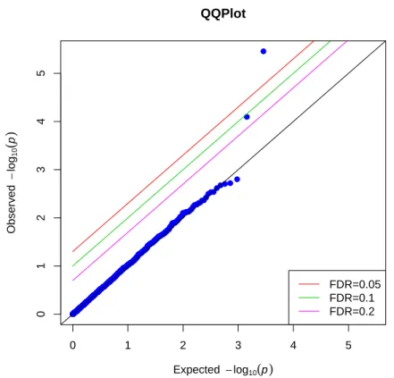
The study enrolled a total of 3263 TMD-free controls and 186 chronic TMD cases. Ge-netic data on 2924 SNPs was available for 3050 of these subjects. The secondary pheno-type for this analysis was the pain density, a quantitative trait calculated as the average self-reported orofacial pain rating (on a 0-100 scale) multiplied by the self-reported per-centage of the day with pain. We included participants with non-missing pain density and all SNPs with a MAF greater than 0.02. The final dataset consists of 3001 patients (with 166 TMD cases and 2835 TMD-free controls) and 2864 SNPs. Using the method described above, principal component analysis was performed on the SNP matrix, and the first 6 components were included in the model as covariates controlling for population stratifica-tion. Gender and dummy variables for OPPERA study sites were also included as covari-ates. The permutation-based IPW procedure was applied to calculate p-values for each SNP as described in Section 3.2.1. The p-values of testing null hypothesis of no associa-tion between pain intensity and a SNP were visualized in Q-Q plot, where under the null hypothesis the p-values were expected to follow uniform distribution.
3.3 Results
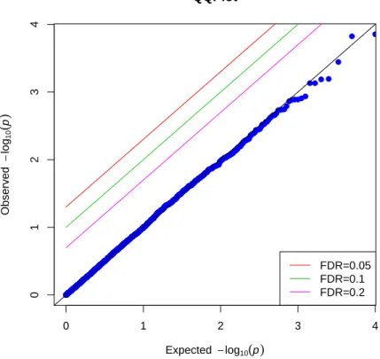
3.3.1 Type I Error
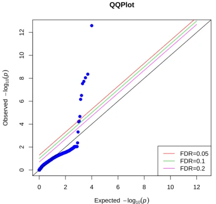
p-values are equal to the observedp-values, and none of the SNP point is above any of the lines corresponding to FDR 0.2, 0.1 nor 0.05. This implies that we do not reject the null hypothesis of no correlation between a “SNP” and secondary phenotype, which is what we expected to see in the simulation. Type I error is well preserved by our nonparamet-ric IPW method in this scenario. While Figure 3.2 is the Q-Q plot of p-values from the same simulated data as those from Figure 3.1, but using conventional IPW method under null hypothesis. We can see that a lot of SNP points’ with obseved p-values largely differ-ent from the expected p-values, even above the lines with FDR 0.05. We rejected the null hypothesis and those SNP points above the line where F DR = 0.05 are significantly
as-sociated with secondary outcome by looking at the plot. However, this is contradictory to our simulated data where none of the SNP is correlated with secondary outcome. This im-plies that conventional IPW method producedd unstable p-values and would inflate type I errors. We cannot use this method in the analysis of real data which are similar to the simulated data, since it would have false positive results and lead to spurious association between them.
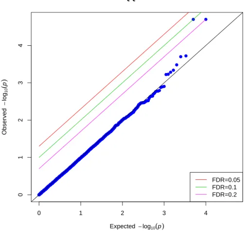
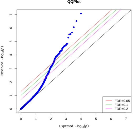
Figure 3.3 and 3.4 showed the p-values for both permutation-based IPW and conven-tional IPW method under null hypothesis when population stratification were considered as illustrated in simulation 2. Similar as the result in simulation 1, almost all the “SNP” points were on the anti-diagonal line where expected p-values were equal to the observed p-values. Only two points were on or above the lines with FDR 0.2and 0.1. None of the
In both simulation scenarios, the p-values produced by conventional IPW regression deviated significantly from the expected p-values, indicating that conventional IPW re-gression is producing anticonservative p-values in these simulation scenarios. In contrast, the distribution of the p-values produced by permutation-based IPW procedure are nearly identical to the expected null distribution. Our method is likely to find out true associa-tion of a SNP and secondary outcome rather than spurious associaassocia-tions which are likely to be produced by conventional IPW method.
3.3.2 Statistical Power
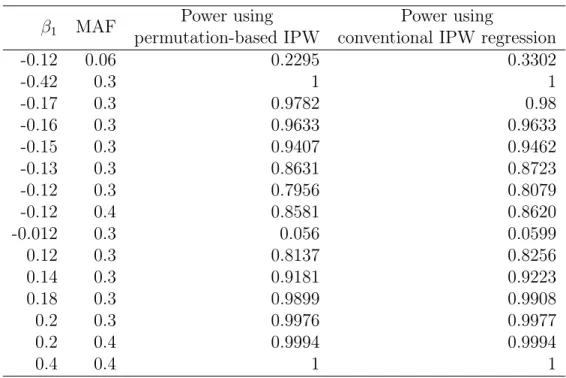
Table 3.1 shows the estimated power of conventional IPW regression and permutation-based IPW approach for various values of M AF and β1. The powers by both methods
were very similar, indicating that our method has comparable power to conventional IPW regression when true association exists.
3.3.3 Data application
3.4 Discussion
IPW regression is a useful tool for evaluating the association between genetic park-ers and secondary phenotypes in GWAS studies. However, it can produce unreliable es-timates when the assumptions of the model, where the secondary phenotype is strongly associated with disease case-control status are violated. In particular, conventional IPW regression performs poorly when evaluating the association between a genetic marker and a secondary phenotype that is equal to 0 for the majority of the controls. IPW regression gives lower weight to cases to account for the fact that they are overrepresented in a case-control study. Thus, if the secondary phenotype is equal to 0 for the majority of case-controls, nearly all of the variance in the secondary phenotype outcome variable occurs among the data with low weight, resulting in unstable regression estimates.
This situation is common in studies of chronic pain such as OPPERA. Suppose we wish to identify SNPs associated with the severity of orofacial pain. All TMD cases have some level of orofacial pain, but the majority of controls report no pain in the orofacial region. If conventional IPW regression is applied to OPPERA (or similar data sets), it produces a large number of anticonservative p-values.
the association between a risk factor and a secondary phenotype.
The proposed method is easy to implement using common statistical software and is relatively fast. Fewer permutations are required when the number of SNPs is large, so the method can be applied to GWAS data sets with millions of markers. Thus, the proposed method is an attractive alternative to conventional IPW regression, particularly for sec-ondary phenotypes with few nonzero values among controls.
Our application to identify SNP’s associated with pain density in TMD case-control studies is also novel. Most previous GWA studies in OPPERA focused on the TMD dis-ease status, which was usually considered as the outcome of interest. Such studies do not consider the fact that the severity of the pain may vary greatly among TMD patients nor the fact that individuals who do not meet the diagnostic criteria for TMD may still expe-rience some levels of pain. Although genetic association of TMD related secondary pheno-type (such as pressure pain sensitivity and non-specific orofacial symptoms) were analyzed in previous studies, our analysis was focusing on pain density and based on candidate genes. This analysis is the first GWA study to identify the association between genetic markers and clinical pain severity, such as pain density. This analysis will lead to the new insights on the genetic risk factors for TMD and chronic pain more generally. In a recent study, Bair et al. (2016) found that TMD consists of at least three homogeneous subgroups or clusters. Some clusters are associated with more severe clinical pain measures. It is be-lieved that patients in different clusters will respond differently to treatments. Identifying genetic markers associated with more severe forms of TMD will hep explaining why some patients have more severe TMD symptoms and may lead to novel treatment plans.