Finite Time Stabilization of Dynamical System with Adaptive Feedback Control

(1)

ISSN Online: 2327-4379 ISSN Print: 2327-4352

Finite-Time Stabilization of Dynamical System

with Adaptive Feedback Control

Zhicai Ma

1

_{, Yongzheng Sun}

2

_{, Hongjun Shi}

2

1_{Department of Mathematics, Longqiao College of Lanzhou University of Finance and Economics, Lanzhou, China} 2_{School of Sciences, China University of Mining and Technology, Xuzhou, China}

Abstract

In this paper, an adaptive feedback controller is proposed to achieve the fi-nite-time stability of dynamical system. In the proposed scheme, the feedback gain of the adaptive feedback controller is automatically tuned according to the adaptation law in order to stabilize unstable fixed points of the system. Based on the Lyapunov function method and the finite-time stability theory, we get a sufficient condition for the finite-time stability. Finally, simulation results show the effectiveness and feasibility of the proposed finite-time con-troller.

Keywords

Chaos, Finite-Time Stabilization, Adaptive Feedback Controller

1. Introduction

In the last two decades, chaos has been a hot topic due to its varied application in many fields, such as information processing, secure communication, power converters, biological system, engineering science, etc. Since Ott, Grebogi, and Yorke (OGY) [1] proposed the first approach of chaos control, and there are many variations reports based on the OGY method [2] [3] [4] [5], creating an entire new research domain in chaos. An important problem in chaos stabiliza-tion is how to design a controller to stabilize the chaotic system. In fact, there is a wide variety of control methods to approach stabilization or synchronization of chaotic systems, including sliding model control [6] [7], adaptive control [8] [9] [10] [11] [12], optimal control [13] [14] and feedback control [15] [16] [17] and other control methods [18] [19][20].

All of the methods mentioned above have been proposed to guarantee the asymptotic stability of chaotic system, but these methods cannot guarantee the How to cite this paper: Ma, Z.C., Sun, Y.Z.

and Shi, H.J. (2017) Finite-Time Stabiliza-tion of Dynamical System with Adaptive Feedback Control. Journal of Applied Ma-thematics and Physics, 5, 412-421. https://doi.org/10.4236/jamp.2017.52036

Received: September 9, 2016 Accepted: February 14, 2017 Published: February 17, 2017

http://creativecommons.org/licenses/by/4.0/

(2)

stability of chaotic systems in a finite time. However, in many cases, we hope the chaotic system achieves stability in a finite time. Finite-time control is a useful technique for achieving finite-time stability. Moreover, the finite-time control technique has been demonstrated better rejection and robustness [21].

Recently, due to its useful applications in many areas, a lot of research work was done about the chaotic system stability based on the finite-time control technique. In Ref. [22], Hong and Wang proposed a continuous finite-time con-trol design method to solve the finite-time stabilization problem for a class of nonlinear control systems and a class of finite-time stabilizing controller for li-near systems appears in [23]. In Ref. [24], the researchers proposed a family of continuous time-invariant finite-time stabilizing controllers for double integra-tor. The most important problem in the study of finite-time chaos stabilization is how to design a physically available and simple controller to guarantee the stabi-lization of chaotic system in a finite time. However, in most of previous studies, the finite-time controller which they choose is too special and complicate to be physically practical. In addition, some of the finite-time controllers have a linear feedback part, but we know that the feedback constant is difficult to find.

Motivated by the above analysis, we propose a physically available and simple adaptive feedback controller to achieve the finite-time stability of chaotic system. Comparing to previous approaches, we employ a time-varying feedback gain in the controller which automatically converges to suitable constants, which make the controller simpler and lead to the speed of asymptotic stability of the system faster. Otherwise, the estimation of the convergence time is also given. The fi-nite-time control technique has demonstrated better disturbance rejection and robustness against uncertainties. Based on the finite-time stability theory and the Lyapunov function method, sufficient condition for finite-time stabilization is obtained. Finally, some numerical examples are examined to illustrate the effec-tiveness of the analytical result.

The rest of this paper is organized as follows. In Section 2, we give some pre-liminary knowledge. In Section 3, the main result is derived based on Lyapunov function method and finite-time stability theory. In Section 4, numerical simula-tions are given to show the effectiveness of the theoretical result. Finally, a con-clusion is drawn in Section 5.

2. Preliminary Knowledge

Consider a dynamical system described by:

( )

,

x t =Ax t + f x t (1)

where

( )

(

( ) ( )

( )

)

T 1 , 2 , ,

n n

x t = x t x t  x t ∈R is the state vector of the dynamical system,

( )

(

( ) ( )

( )

)

T

1 , 2 , , :

n n

n

f x = f x f x  f x R →R is a continuously differen-tiable nonlinear vector function. To stabilize the chaotic orbits in (1) to a fixed point, we consider the adaptive feedback control method. The controlled system (1) can be rewritten as:

( )

,

(3)

where

( )

n

u t ∈R is the input.

Throughout this paper we require the differentiable nonlinear vector function

( )

f x t satisfies the following assumption:

Assumption 1. For function f x

( )

there exists a positive constant l such

that

( )

T

(

( )

)

(

( )

)

( )

T

( )

, , m.

x t −y t f x t − f y t ≤ x t −y t l x t −y t ∀x y∈R

     

        (3)

Remark 1. Condition (3) is usually called global Lipschitz condition, and l

is called Lipschitz constant. It should be pointed out that Condition (3) is very general, most well-known dynamical systems, such as Chua’s circuit, Rössler- like system, Genesio system, and hyperchaotic Lü system, satisfy Assumption

1.

In order to get our main result in the next section, we state here the definition of finite time stability and two lemmas.

Definition 1. System (2) can be finite time stabilized if there exists a constant

0

T> , such that

( ) ( )

lim 0,

t→T x t −s t =

and x t

( ) ( )

=s t if t>T , where T is called the setting time and s t

( )

is a solution of an isolated node, satisfying s t

( )

=As t

( )

+ f s t

( )

.

Lemma 1. [25] Assume that a continuous, positive-definite function V t

( )

satisfies the following differential inequality:

( )

,

V t ≤ −λVβ t

where λ>0, 0<β<1 are all constants. Then, for any given t0, V t

( )

0 satis-fies the following inequality:

( )

(

)(

)

1 1

0 1 0 , ,0 1

V −β t ≤V −β t −λ −β t−t t ≤ ≤t t

and

( )

0, 1,

V t = ∀ ≥t t

with t1 given by

( )

(

)

1 0

1 0 .

1

V t

t t

β

λ β

−

= + −

Lemma 2. [26] Let a a1, 2,,an>0 and 0< <r p. Then

1 1

.

p r

n n

p r

i i

a a

= =

  _≤ 

   



∑

 

∑



3. Main Result

In order to study the finite-time stability of dynamical system (2), we define the synchronization error e t

( )

=x t

( ) ( )

−s t , then the stability of system (2) can be translated into the analysis of the finite-time stability of error system (4). The error system is described by:

( )

.

(4)

In this paper, we designed the controller as follows:

( )

( ) ( )

sign

( )

,

u t = −_k t e t +

η

e t _

(5)

where η is a constant and η≥1,

( )

(

( )

)

(

( )

)

(

( )

)

T

1 2

sign e t = sign e t , sign e t ,, sign e tn  . The feedback gain k t

( )

is adapted according to the following update law:

( )

2

( )

_,

k t = −γe t

(6)

where γ is a arbitrary positive number. In this paper, for a better presentation, we set γ =1, for other cases the extension is straightforward.

Theorem 1. Suppose that the Assumption (1) holds and there exists a sufficiently large positive constant L such that max

( )

s

L> +l

λ

 , where

T

2

s ₌ A+A

 . then

system (2) can be stabilized in a finite-time under the following adaptive feed-back controller (5).

Proof. Take the Lyapunov function

( )

1 _T

( ) ( )

1

( )

2

,

2 2

V t = e t e t + _k t +L_ (7)

where L is a constant bigger that l. Differentiating the function V along the

solution of the system (2),

( )

T

( ) ( )

( )

_.

V t =e t e t +_k t +L k t_

(8)

Substituting e t

( )

and k t

( )

(given by (5) and (6)) into the right-hand of Equation (8), we have

( )

T

( )

2

( )

.

V t =e t _Ae t + f x t − f s t +u t _−_k t +L e t_ (9)

Note that

( ) ( )

( )

( ) ( )

T T

max .

s

e t Ae t ≤

λ

 e t e t (10)

Under Assumption 1, from (5) and (10), we obtain

( )

T

( ) ( )

T

( ) ( )

T

( ) ( )

T

( )

max sign .

s

V t ≤λ  e t e t +le t e t −Le t e t −ηe t e t (11)

Moreover, we notice that T

( )

sign

e t e t = e t , we can get

( )

(

( )

)

T

( ) ( )

( )

max .

s

V t ≤ − L− −l λ  e t e t −ηe t

If max

( )

s

L> +l

λ

 , we have

( )

.

V ≤ −

η

e t

(12)

From Lemma 2, the following inequality is established

( )

1 2 2 1 1 . n n i i i i

e t e t

= =

 

≥ _ _

∑

Thus, we obtain from (12) that

( )

1 1 2 2 2 1 1 2 , n i i

V t η e t η V

=

 

≤ − _ _ −



∑



(5)

where T

( ) ( )

1

. 2

V = e t e t It is to see that V1≤V .

Furthermore, from (13), V is non-increasing. Therefore, there exists a upper

bound V∗, such that

1 .

V ≤ ≤V V∗

Let

( )

1

V t

V

θ = _∗ ≤ _{, then}

( )

t V

( )

t V V1.

θ _≤θ ∗₌

Finally, we have

( )

₂

( )

12 ₂ˆ 12_,

V t ≤ −η θ t V = −η θV (14)

where ˆ _min

( )

t t

θ = θ .

According to Lemma 1, we have

( )

0,

V t ≡ ∀ ≥t T

which further results in

( )

0,

e t ≡ ∀ ≥t T

and the settling time

( )

1 2

0 0

2 , ˆ

V t

T t

η θ

= + ₍₁₅₎

where

( )

_T

( ) ( )

(

( )

)

2

0 0 0 0 2.

V t =_e t e t + k t +L _

  This means that, for any

arbi-trary initial value e t

( )

0 , system (4) can be stabilized by the above controller within the time T. This obviously implies the dynamical system (2) can be sta-bilized by controller (5). This completes the proof. 

Remark 2. In Theorem 1, for the case e t

( )

=0, we assume that k t

( )

≡ −L,

which can guarantee the positive definiteness of the Lyapunov function in (7). In fact, without this hypothesis, the feedback gain k t

( )

will also converge to other suitable constants when e t

( )

=0. Thus, in practical engineering process, the

feedback gain k t

( )

can only adapted according to the updated law in (6). Con-sequently, the design of controller in (5) is independent of the Lipchitz constant of the chaotic system.

4. Simulation Results

In this section, two examples are used to illustrate the feasibility and effective-ness of the above theoretical result.

Example 1: In the first example, we take Chua’s circuit as the first example, which is governed by the following three-dimensional differential equations [27]:

( )

1 1

2

3

0

1 1 1 0 ,

0 0 0

p pb p x x

x x Ax f x

q x

ψ

− −    

 

 

=_ − __{ }+_ _ +

 ₋    

    

(6)

where

(

)

T 3 1, 2, 3

x= x x x ∈R is the state vector,

( )

x1 0.5p b a

(

)(

x1 1 x1 1 .

)

ψ

= − + − − _{In all of the simulations, we always choose} the system parameters of the Chua’s circuit as p=10, 14.87, 1.27,q= a= − ,

0.68

b= − which causes the Chua’s circuit to exhibit a double-scroll chaotic at-

tractor. It is easy to compute that max T 7.857

2

A A

λ _ + _=

  . Take

( )

s 2.95

(

s 1 s 1

)

ϕ

= + − − _{. It is easy to verify that}

ϕ

( ) ( )

s₁ −

ϕ

s₂ ≤ s₁−s₂ .

Applying (16) we have

(

)

(

( )

)

(

)(

) ( )

(

( )

)

(

)(

) (

)

T

1 1 1 1

T

.

x y f x f y p b a x y x y

p b a x y x y

ϕ ϕ

− − = − − −

≤ − − −

Therefore the Assumption 1 is satisfied with l= p b

(

−a

)

=5.9. Here we take 14

L= , it is easy to see the condition max

( )

s

L> +l

λ

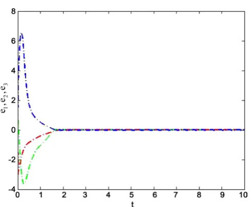
 is satisfied. Take η=1, we simulate the evolution of the system (16) according to the controller defined in (5). According to Theorem 1, system (2) can be stabilized in a finite time. Figure 1 shows the temporal evolution of the Chua’s circuit, where the initial values of the system are taken as

(

1, 3, 2−

)

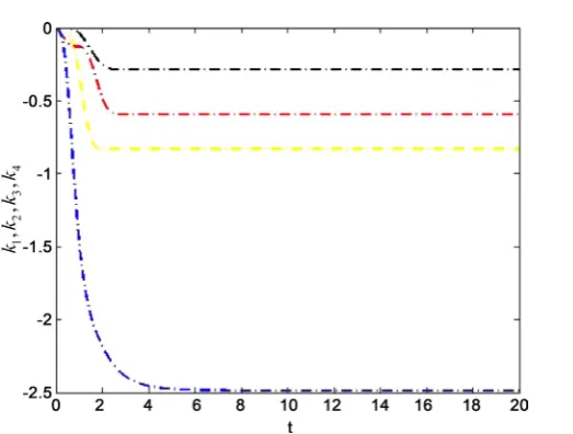
, respectively. By computing (15) with

matlab, we get T =1.7864. It can be observed that the finite-time stable is achieved successfully by the proposed control scheme (5). The simulation matches the theoretical result perfectly. The temporal evolutions of variable strengths

(

1, 2, 3

)

i

k i= are also simulated in this paper, the initial values are set as zero. From Figure 2 we can see that feedback strengths ki reach some certain

con-stants when the system is stabilized.

Example 2: To show the generality of the presented method, the second ex-ample is the hyperchaotic Rössler system [28]:

( )

1

2

3 1 3

4

0 1 1 0 0

1 0 1 0

,

0 0 0 0

0 0 0

x x

x Ax f x

x x x

x α θ δ ζ −                   =_ __{ }+_ _ + +    ₋        

  (17)

where

(

)

T ₄

1, 2, 3, 4

x= x x x x ∈R is the state vector.

The system has a hyperchaotic attractor with two positive Lyapunov expo-nents. Similarly, for the hyperchaotic Rössler system, we choose the initial con-ditions of the system (2) are rand but the feedback strengths ki are set as zero.

The system parameters set as α =0.25, δ =0.5, ζ =0.05 and

θ

=3. Figure 3 shows the temporal evolution of hyperchaotic Rössler system, and Figure 4 shows the temporal evolutions of the corresponding feedback strengths ki. From

Figure 3 one can find that the system (17) can be achieved stabilization within a finite time under the controller of (5).

The above numerical examples show that the stabilization of chaotic or hyperchaotic system can be quickly achieved by the present controller in the form of (5). In addition, we also simulated the time-varying feedback gains ki,

(7)

[image:7.595.252.498.63.265.2] [image:7.595.252.494.296.483.2]

Figure 1. Trajectories of the Chua’s circuit system with adaptive controller (5).

Figure 2. Feedback strength k ii

(

=1, 2,3

)

of adaptive controller (5) for dynamical sys-tem (2).

[image:7.595.251.494.528.717.2]

(8)

[image:8.595.252.514.61.259.2]

Figure 4. Feedback strength k ii

(

=1, 2,3, 4

)

of adaptive controller (5) for dynamical system (2).

corresponding feedback signals, we find that the coupling is indeed small in the above two examples.

5. Conclusion

In this paper, we have investigated the stabilization of chaotic system based on the finite-time stability theory of differential equations, and proposed a simple, systematic and rigorous adaptive feedback control method to stabilize finite- dimensional chaotic systems within a finite time. In comparison with previous methods, the proposed scheme is simple to implement in practice. Numerical simulations are provided to illustrate the effectiveness of the method. The present study does not consider the effect of time delays, however, research is being pursued in this direction.

References

[1] Ott, E., Grebogi, C. and Yorke, J.A. (1990) Controlling Chaos. Physical Review Let-ters, 64, 1196-1199. https://doi.org/10.1103/PhysRevLett.64.1196

[2] Boccaletti, S., Grebogi, C., Lai, Y.C., et al. (2000) The Control of Chaos: Theory and Application. Physical Report, 329, 103-197.

https://doi.org/10.1016/S0370-1573(99)00096-4

[3] Yang, L., Liu, Z.R., Mao, J.M. (2000) Controlling Hyperchaos. Physical Review Let-ter, 84, 67-70. https://doi.org/10.1103/PhysRevLett.84.67

[4] Singer, J., Wang, Y.Z. and Bau, H.H. (1991) Controlling a Chaotic System. Physical Review Letter, 66, 1123-1125. https://doi.org/10.1103/PhysRevLett.66.1123

[5] Auerbach, D., Grebogi, C., Ott, E., Yorke, J.A. (1992) Controlling Chaos in High Dimensional Systems. Physical Review Letter, 69, 3479-3482.

https://doi.org/10.1103/PhysRevLett.69.3479

[6] Yan, J., Hung, M., Chiang, T. and Yang, Y. (2006) Robust Synchronization of Chao-tic Systems via Adaptive Sliding Mode Control. Physical Letter A, 356, 220-225.

https://doi.org/10.1016/j.physleta.2006.03.047

(9)

of Two Different Uncertain Chaotic Systems with Unknown Parameters Using a Robust Adaptive Sliding Mode Controller. Communications in Nonlinear Science and Numerical Simulation, 16, 2853-2868.

https://doi.org/10.1016/j.cnsns.2010.09.038

[8] Huang, D.B (2005) Simple Adaptive-Feedback Controller for Identical Chaos Syn-chronization. Physical Review E, 71, 037203.

https://doi.org/10.1103/PhysRevE.71.037203

[9] Chen, X. and Lu, J. (2007) Adaptive Synchronization of Different Chaotic Systems with Fully Unknown Parameters. Physical Letter A, 364, 123-128.

[10] Lei, Y.M. and Xu, Y. (2009) Adaptive Synchronization of an Uncertain Qi System via Only One Scalar Controller. Physica Scripta, 79, 065008.

https://doi.org/10.1088/0031-8949/79/06/065008

[11] Park, J.H. (2007) Exponential Synchronization of the Genesio-Tesi Chaotic System via a Novel Feedback Control. Physica Scripta, 76, 617-622.

https://doi.org/10.1088/0031-8949/76/6/004

[12] Lin, W. (2008) Adaptive Chaos Control and Synchronization in Only Locally Lip-schitz Systems. Physical Letter A, 372, 3195-3200.

[13] Cheng, S., Ji, J.C. and Zhou, J. (2013) Fast Synchronization of Directionally Coupled Chaotic Systems. AMathematical Modelling. 37, 127-136.

https://doi.org/10.1016/j.apm.2012.02.018

[14] Ma, J., Zhang, A., Xia, Y. and Zhang, L. (2010) Optimize Design of Adaptive Syn-chronization Controllers and Parameter Observers in Different Hyperchaotic Sys-tems. Applied Mathematics and Computation, 215, 3318-3326.

https://doi.org/10.1016/j.amc.2009.10.020

[15] Liu, D.S. and Yan, G.Z. (2013) Stabilization of Discrete-Time Chaotic Systems via Improved Periodic Delayed Feedback Control Based on Polynomial Matrix Right Coprime Factorization. Nonlinear Dynamics, 74, 1243-1252.

https://doi.org/10.1007/s11071-013-1037-y

[16] Faieghi, M., Kuntanapreeda, S., Delavari, H. and Baleanu, D. (2013) LMI-Based Sta-bilization of a Class of Fractional-Order Chaotic Systems. Nonlinear Dynamics, 72, 301-309. https://doi.org/10.1007/s11071-012-0714-6

[17] Li, N., Yuan, H.Q., Sun, H.Y. and Zhang, Q.L. (2013) An Impulsive Multi-Delayed Feedback Control Method for Stabilizing Discrete Chaotic Systems. Nonlinear Dy-namics, 73, 1187-1199. https://doi.org/10.1007/s11071-012-0434-y

[18] Sun, J.W., Wang, Y.F., Yao, L.N., Shen, Y. and Cui, G.Z (2015) General Hybrid Projective Complete Dislocated Synchronization Between a Class of Chaotic Real Nonlinear Systems and a Class of Chaotic Complex Nonlinear Systems. Applied Mathematical Modelling, 39, 6150-6164. https://doi.org/10.1016/j.apm.2015.01.049

[19] Khan, A. and Singh, P. (2015) Chaos Synchronization in Lorenz System. Applied Mathematical Modelling, 6, 1864-1872. https://doi.org/10.4236/am.2015.611164

[20] Aziz, M.M. and AL-Azzawi, S.F. (2016) Control and Synchronization with Known and Unknown Parameters. Applied Mathematical Modelling, 7, 292-303.

https://doi.org/10.4236/am.2016.73026

[21] Bhat, S.P. and Bernstein, D.S. (2000) Finite-Time Stability of Continuous Auto-nomous System. SIAM Journal on Control and Optimization, 38, 751-766.

https://doi.org/10.1137/S0363012997321358

(10)

of Nonlinear Systems. Science in China Series F, 49, 80-89.

https://doi.org/10.1007/s11432-004-5114-1

[23] Salehi, S.V. and Ryan, E.P. (1982) On Optimal Nonlinear Feedback Regulation of Linear Plants. IEEE Transactions on Automatic Control, 27, 1260-1264.

https://doi.org/10.1109/TAC.1982.1103108

[24] Rang, E.R. (1963) Ioschrone Families for Second-Order Systems. IEEE Transactions on Automatic Control, 8, 64-65. https://doi.org/10.1109/TAC.1963.1105520

[25] Feng, Y., Sun, L.X. and Yu, X.H. (2004) Finite Time Synchronization of Chaotic Systems with Unmatched Uncertainties. The 30th Annual Conference of the IEEE Industrial Electronics Society, Busan, Korea, 2004, 2911-2913.

https://doi.org/10.1109/iecon.2004.1432272

[26] Hardy, G., Littlewood, J. and Polya, G. (1952) Inequalities. Cambridge University Press, Cambridge.

[27] Chua, L.O., Wu, C.W. Huang, A. and Zhong, G.Q. (1993) A Universal Circuit for Studying and Generating Chaos I: Routes to Chaos. IEEE Transactions on Circuits and Systems,I: Fundamental Theory and Applications, 40, 732-744.

https://doi.org/10.1109/81.246149

[28] Rossler, O.E. (1979) An Equation for Hyperchaos. Physics Letters A, 71, 155-157.

https://doi.org/10.1016/0375-9601(79)90150-6

Submit or recommend next manuscript to SCIRP and we will provide best service for you:

Accepting pre-submission inquiries through Email, Facebook, LinkedIn, Twitter, etc. A wide selection of journals (inclusive of 9 subjects, more than 200 journals)

Providing 24-hour high-quality service User-friendly online submission system Fair and swift peer-review system

Efficient typesetting and proofreading procedure

Display of the result of downloads and visits, as well as the number of cited articles Maximum dissemination of your research work