Munich Personal RePEc Archive
On the stability of the Ramsey
accumulation path
Bellino, Enrico
28 January 2013
Online at
https://mpra.ub.uni-muenchen.de/44024/
On the stability of the Ramsey accumulation path
1 Enrico Bellino2December 4th, 2012 – forthcoming inLevrero S., Palumbo A. and Stirati A. (eds.), Sraffa and the Reconstruction of Economic Theory, Vol. 1, Theories of Value and Distribution, Palgrave Macmillan, Houndmills, Basingstoke, Hampshire, UK, 2013.
Abstract The Ramsey (1928) accumulation path is characterized as a saddle-path in the standard presentations of the model based on the works of Cass (1965) and Koopmans (1965). From a mathematical stance a saddle-path is unstable: if the system is exactly on that path, it converges to the steady state of the system; if it diverges slightly from that path, it shifts indefinitely from the steady state. The ‘transversality’ condition is then invoked in the Ramsey model to prevent the system from following such divergent paths; from the economical point of view this condition can be interpreted as a perfect foresight assumption. This kind of instability, which is typical of infinite horizon optimal growth models, has been sometime considered to account for actual economic crises. The claim would seem to be grounded on the idea that if the consumer optimizes myopically, i.e., by only considering the current and the subsequent period, the ensuing dynamics diverges almost surely from the steady state equilibrium. Convergence requires perfect foresight.
The present work aims to challenge this conclusion, which seems not inherent to the choice problem between consumption and savings, but it is due to the presumption that the consumer must face this problem in an infinite horizon setting. The Ramsey problem of selection of the accumulation path will be re-proposed here within a framework where consumer’s ability to optimize over the future is assumed to be imperfect. However, the ensuing path will converge to the steady state, without assuming perfect foresight. Myopia is thus not ultimately responsible for the instabilities of the ‘optimal’ accumulation path. Explanations of instability phenomena of actual economic systems (crises, bubbles, etc.) must be sought in other directions, probably outside the strait-jacket of the optimization under constraint.
1. Introduction
Infinite horizon Neoclassical optimal accumulation theory is characterized by an analytical apparatus that has now pervaded several fields of theoretical analysis: capital theory, growth and value theory, macrodynamics, ecc. In this context the equilibrium solutions take the form of saddle-paths which are, therefore, unstable paths. The convergence of these solutions to the steady state equilibrium is then ensured by imposing a transversality condition, that is, a condition which guarantees the optimality of the solution when time tends to infinity.
1
The material presented in this paper is fruit of a set of discussions stimulated by Pierangelo Garegnani on the meaning of the ‘transversality condition’ within optimal capital accumulation models. I am sincerely grateful for having had these discussions with him. In addition, I wish to thank Andrea Battinelli, Carlo Beretta, Marco Bramanti, Thomas Christiaans, Roberto Ciccone, Ferdinando Colombo, Saverio Fratini, Kazuhiro Kurose, Enrico Sergio Levrero, PierCarlo Nicola, Fabio Petri, Mario Pomini, Neri Salvadori, Paolo Trabucchi, Alessandro Sbuelz, Gerd Weinrich and an anonymous referee for their comments and suggestions on earlier versions of this work. However, the responsibility of what is written here is entirely mine. Finally, I am grateful to Micaela Tavasani, for English revision.
2
2
Sometimes, this kind of dynamics has been considered to account for the crises of actual economic systems. A quite recent work supporting this position is proposed by Christopher Bliss:
Question: Which Cambridge, England, paper of the 1960s or 1970s did more damage to simple neoclassical thinking than any other? I can imagine the post-Keynesians proposing one or more papers by Joan Robinson, but I would not agree. My own candidate would be Frank Hahn’s 1968 paper on warranted growth paths. What Hahn did can be explained quite simply. [...] In general, equilibrium conditions for the various capital goods—that is, equal net returns for each good—depend upon the rate of change of prices, not just on the prices alone. Then the intertemporal dynamic equilibrium of the system is defined by a set of simultaneous differential equations. What can we say about those equations? The easiest route to the answer comes from the theory of optimal growth, as with a many-capital-good Ramsey model. From there we obtain dynamic equilibrium conditions (Euler equations), but these do not suffice by themselves. We need to add transversality conditions. The dynamic equations are of the saddle-point variety. Only transversality ensures that the system converges to the right asymptotic state. Hahn, following a suggestion from Mirrlees, realized that a non-optimized dynamic equilibrium is just like the necessary conditions for an optimized system. There will be infinitely many ‘equilibrium’ paths for prices, but most of these will crash into the sign-constraint barriers of the race track.
In other words, a successful capitalist economy needs to have the right idea of where it should go in the long run. It would be hard to imagine a more telling criticism of the theoretical claim that an ideal decentralized capitalist system exhibits optimal properties. For if there is one thing that capitalist economies are really bad at, it is knowing where they are going in the long run and judging that destination correctly. Recent financial crises, and similar crises in the past, remind us that capitalism is like an inexperienced child that chases after the latest shiny attraction until it hurts itself and ends up in tears (Bliss, 2010, pp. 648-9).
This quotation hints at several related issues, sometime mixed up; roughly, Bliss seems to suggest that Neoclassical optimal accumulation models aim to account for both the equilibrating and the destabilizing forces of capitalist economies. He seems to say that crises in actual capitalist economies can be explained, at least partially, by the destabilizing forces implicit in Neoclassical optimal growth theory. At a deeper level, this claim would seem to be grounded on the idea that if the consumer optimizes myopically, i.e., by considering only the current and the subsequent period, the ensuing dynamics diverges almost surely from the steady state equilibrium. On the contrary, convergence to the steady state equilibrium requires consumer’s perfect foresight. Myopic optimization, in other words, would be actually the ‘responsible’ for the instabilities, while long-run foresight is the assumption that guarantees the convergence of short run or momentary equilibria towards a steady state. An interesting analysis of the role of consumer foresight ability in connection with the dynamic properties of the optimal accumulation path is proposed by Heller3:
It is a curious fact that while most finite time horizon economic models are stable, almost all infinite time horizon models are unstable. ... Hahn [Q.J.E., 1966 and R.E.S., 1968, e.b.] and Shell-Stiglitz [Q.J.E., 1967, e.b.] cast considerable doubt for simple ‘descriptive’ economic models that efficient equilibrium paths are ever chosen by myopically optimizing, competitive agents when there is no end to time. In Ramsey planning models, there is a similar instability: if central planners initially choose the right path, minor external shocks could cause them to follow a non-optimal path when they operate according to
3
3
myopic optimization rules ... It may be helpful to spell out this point a bit further. The infinite horizon models of Hahn and others restrict attention to momentary equilibrium paths arising from arbitragers possessing self-fulfilling expectations about price changes in the immediate future (we will call this myopic foresight). A path is in equilibrium at a moment in time if, given current prices and myopic foresight expectations about prices in the immediate future, agents make plans about the allocation of resources across consumption and various investment goods that clear markets at the current moment. Paths that are in equilibrium for non-infinitesimal lengths of time, but are not necessarily in equilibrium for all time, are called momentary equilibrium paths. Paths that are in equilibrium at every moment in time are called long run equilibrium paths. Momentary equilibrium paths need not be long run equilibrium paths because, for example, the stock of some capital good is run down to zero at some point, resulting in a disequilibrium at that time (Heller, 1975, pp. 65-6).
In these pages I aim to challenge the idea that myopic optimization is ultimately responsible for instability and that the assumption of perfect foresight is the only way to avoid it. In this work we will limit our investigation to an optimal accumulation model with just one
good, in order to focus on the causes of instability in the simplest situation in which it emerges. We will study a myopic adjustment process compatible with consumer rational behaviour; the ensuing accumulation path will be proved to converge monotonically to the Ramsey steady state equilibrium. The extension to the cases with more than one good, which are those considered by Hahn and referred to by Bliss, will be undertaken in a subsequent work.
2. Setting of the Cass-Koopmans-Ramsey model
Let us consider what the (representative) consumer has to do in order to discover his optimal consumption path over an infinite time horizon. Consider an economic system where just one commodity is produced, consumed and employed jointly with labour as a mean of production of itself; capital depreciates at rate [0, 1]. We define period t the half-open time interval [t, t + 1) between dates t and t + 1. Consumers live forever, and they are all equal. We can thus study the behaviour of the representative consumer. To simplify, let us suppose that population remains constant. Time is considered a discrete variable, making it easier to analyse the situation as a sequence of events4. Consumer’s preferences have a cardinal
representation, 5 being described by an utility functional,
0 = 1
1 ( )
= t t
t
c u
U , constituted by a
sum of discounted utilities achieved in each period, u(ct), where ct is the consumption level in
period t,6
1
1 is the discount factor of future utility and > 0 is the rate of time preference.
We suppose that u : R+ → R is a twice continuously differentiable, increasing and concave function; hence u(ct) > 0 and u(ct) < 0; by simplicity, let’s assume also limct0u'(ct) = +.
Technology is described by the per-capita production function, f(kt), where f(kt) is the flow
of per worker gross output (gross of capital replacements) and kt is the per worker flow of
4
For discrete time versions of the Ramsey model see, for example, Azariadis (1993, Chaps. 7 and 13) or Stockey and Lucas (1989, Chap. 2).
5
See Koopmans (1965, Section I); see also Hicks (1965, Chap. XXI, in particular pp. 256-7 and Appendix E). 6
4
services from the real capital stock. f : R+ → R+ is a twice continuously differentiable, increasing and concave function; hence f(k) > 0 and f (k) < 0. Moreover, f(0) = 0,
) ( lim
0 f k
k = + and limk f(k)= 0
+
.
Now, let’s analyse the ‘centralized’ solution, i.e., the consumption path maximizing consumer utility over the whole period considered:
( )=
max 11
0 = } ,
{ t
t
t k
ct t U u c
,where
ct = f(kt) – kt – (kt+1 – kt), t = 0, 1, 2, ..., (Ct)
and
0 0 =k
k ,
where k0 is the (given) initial capital endowment per worker.
As regards the meaning of the physical constraint (Ct) kt observe that, without loss of
generality, we can assume that each unit of capital provides a unitary flow of capital service within the period, so that the same symbol kt denotes the per worker flow of services from the
real capital stock (when it appears as argument of function f) and the per-worker capital stock
available at date t, that is, at the beginning of period t. On the other hand, f(kt) – kt and ct are
the flows of net product per worker and of consumption per worker during period t (‘yearly’ flows). Suppose that within each period a uniform flow of net output and of consumption is made available by the production process (a ‘daily’ flow); in this way the contemporaneity between production and consumption entailed in (Ct) does not raise problems from the logical point of view.7 Moreover, suppose that the new capital accumulated during period t starts to
generate capital services only with the beginning of the subsequent period (‘time do build’ assumption); in this way we can disregard the formation of new capital during the period.
Let’s suppose thatk0 <k~, where k~ is that level of capital labour ratio which makes the net product per worker equal to zero, i.e.
k k
f(~)~. (1)
7
Alternatively we could express the physical constraint in the form
ct+1 = f(kt) – kt – (kt+1 – kt), t = 0, 1, 2, ...; (Ct)
5 The optimal path of consumption8c
t, with t = 0, 1, 2, 3,... and of capital, kt, with t = 1,
2, 3, ... can be found as follows:9 at the beginning of each period t the stock of capital, k
t, is
determined by past saving decisions. After substituting the physical constraints (Ct) in the utility functional, there are just two addenda that include kt+1:
[ ( ) ]= 1 1 = 1 0 =
u f k k k k
U 1 2 1 1 1 1 ) (1 ] ) ( [ ) (1 ] ) ( [ t t t t t t t t t
t k k k u f k k k k
k f u .
Derive U with respect to kt+1 and set the result equal to zero; after simplifying we have:
... , 2 , 1 , 0 , 1 1 ) ( ] ) ( [ ] ) ( [ 1 2 1 1 1
1
t k f k k k k f u k k k k f u t t t t t t t t t
; (Ut)
and re-substituting (Ct) and (Ct + 1) we obtain:10
, 1 ] ) ( 1 [ ) ( = )
( 1 1
t t
t k f c u c
u t = 0, 1, 2, .... (UCt)
To understand the economic meaning of conditions (UCt), consider the consumption allocation problem faced by the representative consumer between periods t and t + 1. If the consumer decreases consumption in period t by dct, the ensuing loss of utility is u(ct)dct. This
decrease in consumption of period t allows for more accumulation: gross output of period
t + 1 increases by f(kt+1)dct. Consumption of period t + 1 may be increased by [ f(kt+1) –
+ 1]dct, including what is left of the initial amount of capital invested. This will increase
utility of period t + 1 by u(ct+1)[ f(kt+1) – + 1]dct. Along the optimal path these (small)
reallocations of consumption must leave welfare unchanged: the loss in utility of period t
must compensate the discounted increase of utility of period t + 1, that is:
u(ct)dct = .
1 d 1] ) ( )[
( 1 1
ct f kt ct u
8
Throughout the work consumption is intended as consumption ‘per worker’; the same can be said for net product, saving and capital. For the sake of brevity, we will omit this specification.
9
Here we follow closely Azariadis (1993, § 7.3 and § 13.4); for the more usual continuous time case see Blanchard and Fischer (1989, § 2.1).
10
A similar condition can be obtained for the continuous case; see, for example, Blanchard and Fischer (1989, § 2.1). By writing the physical constraint in the form (Ct), conditions (Ut) would remain unaltered, with the only difference that now the arguments of the marginal utilities at the left-hand and at the right-hand are now ct+1 and ct+2; consequently conditions (UCt) take the form
, 1 ] ) ( 1 [ ) ( = )
( 2 1
1
t t
t k f c u c
6
After simplification we obtain equations (UCt). The left-hand and the right-hand members of (UCt) could be called ‘marginal utility of consumption’ and ‘marginal utility of savings’. It is to be noted that the optimization process entailed by condition (UCt) concerns just two periods at a time: t and t + 1. The integral consumption of what remains of the additional capital transferred from period t to t + 1 sterilizes any effect of this capital accumulation for periods t + 2, t + 3, ecc. This allows us to focus just on costs and benefits for periods t and
t + 1. No costs and benefits due to reallocations between periods t and t + 1 arise for t + 2, t + 3, ...; otherwise these effects should have been taken into account in identifying the optimal intertemporal allocation.
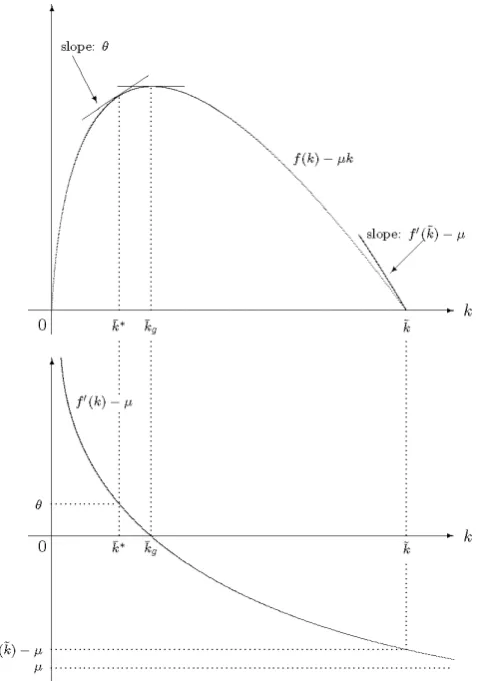
Physical constraints (Ct) and the ‘equi-marginality’ equalities (UCt) are necessary conditions to select the optimal behaviour of the representative consumer. The steady-state of the system (UCt)-(Ct) is represented by the pair (k*, c*), where k* is that value of k such that
f (k*) = + (2)
and c* = f(k*) – k*. Equation (2) is called the ‘modified golden rule’, as it differs from the traditional ‘golden rule’,
f (kg) = , (3)
which is the condition to select the capital labour ratio, kg, that maximizes the net product per
worker, f(k) – k. As f is decreasing we have
. ~ < <
*
k k
k g
7
Figure 1. Net product, f(k) k, and its derivative, f (k)
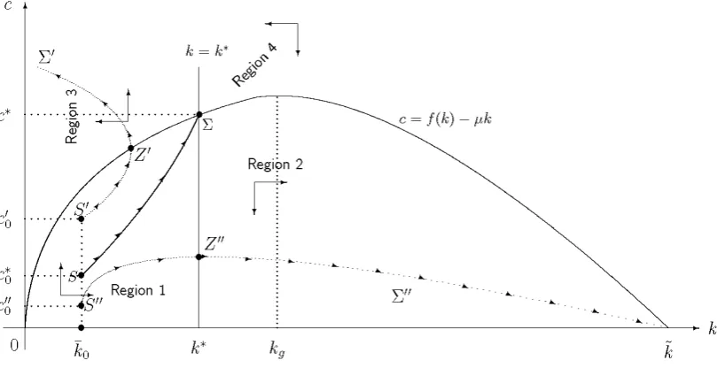
3. Excluding divergent paths: the transversality condition
The dynamics described by equations (UCt) and (Ct) can be analysed by the phase portrait represented in Figure 2. The curves f(k) – k and k = k* divide the positive quadrant in four regions: 1, 2, 3 and 4. The direction of the movement in each of these regions is described by the small arrows: by (Ct) we deduce that kt+1 <> kt if and only if ct <> f(kt) – kt; by (UCt) we
deduce that ct+1 <> ct if and only if kt <> k*. The direction of arrows suggest that the dynamics of
kt and ct is a saddle path, that is, an unstable path. The cause of this instability lies in the
peculiar way in which the initial consumption level, c0, is selected. Let us focus on this
procedure, step by step. At date t = 0 equations (U) and (C) become
1
) ( 1
) ( = )
( 1
1 0
k f c
u c
8
) (
) (
= 0 0 1 0
0 f k k k k
c (C0)
) (
) (
= 1 1 2 1
1 f k k k k
c (C1)
We have thus three equations in four unknowns: c0, k1, c1 and k2; one of them must be fixed
from outside. In infinite horizon models c0 is initially chosen arbitrarily and then one looks if
this choice is compatible with utility maximization in the long run. Suppose that k0 <k*;
hence [1 + f(k0)]/(1 + ) > 1. If c0 is initially fixed at a high level, not too far from the
net product f(k0)k0 (like, for example, c0 in Figure 2), the first member of (U0) will be
quite low (since u is decreasing); on the other hand (C0) determines k1 not too far from k0
and thus the ratio [1 + f (k1)]/(1 + ) will remain close to [1 + f(k0)]/(1 + ), and
thus higher than 1. Hence, in order to align the r.h.s. of (U0) with the low level reached by )
(c0
u , future consumption must be fixed at a level higher than c1, i.e., c1>c0. In other words, given a high initial consumption level, to ‘justify’ (rationalize) this choice future consumption must be fixed at an even higher level. Analogous adjustments, all entailing an ever increasing consumption in periods t = 2, 3, ... will take place, up to the point where capital is totally devoured! This is what happens along the S path of the Cass-Koopmans diagram (see Figure 2): initial consumption is kept fixed at c0 and ct is increased (savings are
decreased) in all subsequent periods; from point Z on, besides consuming the entire net product of each period, the individual starts ‘eating’ away the capital stock, until it is dragged to 0.
If, on the other hand, initial consumption is fixed at a low level, like c0 in Figure 2, then
) (c0
u will be quite high and (C0) will determine k1 at a level which is significantly higher
than k0, so that the ratio [1 + f (k1)]/(1 + ) will be significantly lower than [1 +
) (k0
f ]/(1 + ). In order to keep the r.h.s. of (U0) at the high level of u(c0) future consumption cannot be fixed at a very high level, in spite of the large accumulation that has just taken place. This leaves a large amount of resources for accumulation, pushing the system into an over-accumulation path, like S in Figure 2, where consumption starts decreasing from point Z onwards where k > k*, thus making the net marginal productivity of capital fall below the factor of time preference. The system is thus dragged to point (k~, 0) where the entire gross product f(k~) is devoted to the maintenance of capital, k~: the initial error, of a too low initial consumption level, is thus corrected by low levels of future consumptions – which decrease even to zero from a certain point onwards!
It can be proved that there is only one level of initial consumption, c0, that places the consumer on his optimal intertemporal path. All other levels of c0 lie in an over-consumption
9
Figure 2. Phase portrait of the Cass-Koopmans-Ramsey model
In both examples, initial consumption is taken as given; this is just a provisional assumption, an analytical device that shows that almost all levels of initial consumption lie on a divergent path: infinitely many divergent paths, like S, or S, can be obtained along which the adjustments, necessary for rationalizing the ‘error’ of fixing an arbitrary level of c0, are
shifted to future changes, rather than changes in present consumption. These instability phenomena are then amended by introducing a further condition, the so-called ‘transversality condition’, that excludes all diverging paths like S or S. In formal terms it is represented by
0. = 1
1 ) ( lim
t
t t t
c u
k
(T)
In all divergent paths ct would become 0, sooner or later, hence u(c) tends to infinite. This
eventuality is excluded by condition (T). But, even if formally correct, this procedure seems to miss the economic substance of the problem. Why should a consumer who wants to optimize his consumption plan commit himself to keeping c0 fixed? In his utility
maximization problem c0 is surely the first variable he will adjust. Obviously, it is not the
only variable to consider; rather, he must adjust the whole stream of future consumptions, i.e., infinitely many consumption levels (c0 included)! But while this problem is handy in the
finite horizon case11, at least in principle, it seems quite difficult or even unsolvable in the
11
10
infinite horizon case. The selection of the saddle path entails, from the logical point of view, the solution of infinitely many optimization problems: for any given c0 the whole path of pairs
(kt, ct) satisfying conditions (UCt) and (Ct) should be calculated; when we realize that it
diverges from the steady state—and this will be the case for all but one path—we have to calculate another path starting from another level of c0. In this way we would select the
unique path converging to the steady state. But this would require almost unlimited computational power for the consumer concerning present and future consumptions and savings. In other terms, it requires long-run or perfect foresight.
Moreover, this way of selecting the optimal path introduces an instability phenomenon which is not inherent to the optimization problem we are studying. It is due both to the presumption that the consumer must face an infinite horizon optimization problem and to the analytical tools available to solve such problem. The crucial difficulty consists in the fact that a rational choice of c0 would require at the same time choosing the whole future path ct, t = 1,
2, 3, .... As this problem is not directly solvable we must resort to the indirect way to fix arbitrarily c0 and check later on if the ensuing path converges or diverges. The extraordinary
high computational power so required to the consumer makes the model extremely unrealistic. Moreover, it conveys the wrong idea of a structural instability of the long run accumulation path, only remediable by assuming consumer perfect foresight.
In what follows, an alternative way of selecting the optimal accumulation path is proposed, which requires a considerably reduced foresight ability for the consumer. If we realistically limit to assume that in each period the consumer is able to balance the marginal effects of reallocations over a finite number of periods, we obtain a path convergent to the steady state
1
] ) ( 1
[ ) ( = )
( 1 1
0
k f c
u c u
1
] ) ( 1
[ ) ( = )
(c1 u c2 f k2 u
) ( )
(
= 0 0 1 0
0 f k k k k
c
) ( )
(
= 1 1 2 1
1 f k k k k
c
) ( )
(
= 2 2 3 2
2 f k k k k
c
We have 5 equations in 6 unknowns: c0 , c1 , c2 , k1 , k2 , and k3. A further equation is required to cap the degree of freedom. One possibility is to impose the total exhaustion of capital at the end of the planning period, i.e.,
0. =
3
k
11
that is optimal within the set of constraints imposed on the consumer’s ability to optimize over the future. Obviously, it is necessarily sub-optimal if compared with the saddle path, being the result of a set of optimizations defined over a more restrictive set of constraints but, ‘better is the enemy of good’, as an Italian proverb states. A set of scenarios can thus be outlined where perfect foresight is no longer necessary to exclude divergent paths: myopic optimizing rules are compatible with the convergence to the steady state.
4. An alternative approach: adjustments towards the optimal path
Given
* 0 0 =k <k
k (4)
one possible choice, that the consumer can adopt, is to consume the entire net product in each period. By (Ct) we see that this choice is feasible and entails
0 1=k =k
kt t and ct = f(k0)k0 for any t = 0, 1, 2, ... . (Y0-) This is not a unique option and probably not the optimal one. It is a provisional choice12 that
can be used as a starting point to begin fixing ideas.
In this situation, consider the intertemporal re-allocation constituted by (a) and (b) below: (a) in period t = 0 save and invest 1 unit of the good;
(b) the unit saved in period t = 0 results in
(k0)
f (5)
units of additional net product in all future periodst = 1, 2, 3,.... The effects of (a) and (b) on consumer’s welfare are:
(A) a loss of utility for saving 1 unit in period t = 0 given by13
1 ] ) (
[ 0 0
f k k
u , (6)
(B) a utility gain ensuing from consuming the additional net product (5) in all future periodst
= 1, 2, 3, ... In each period this utility gain is
]. ) ( [ ] ) (
[ 0 0 0
f k k f k
u (7)
The flow of utility gains (7) arising from the additional consumption in all future periods t = 1, 2, 3, ... discounted at t = 0 is
...
3 ) (1
] ) ( [ ] 0 ) 0 ( [ 2
) (1
] ) ( [ ] 0 ) 0 ( [ 1
] ) ( [ ] 0 ) 0 (
[ 0 0 0
k f k u f k k f k u f k k f k k
f u
12
In what follows, a provisional value assumed by a certain variable is denoted by apex ° and the definitive value assumed by that variable by apex •.
13
12 ] [ ( ) ] ( ) = [ ( ) ] [ ( ) ] ) ( [
= 0 0 0
11 1 = 0 0 0
f k k f k
u f k k f ku t
t
(8)
(notice that all relevant functions in (6), (7) and (8) are evaluated at the levels of capital services per worker and of consumption per worker planned through (Y0-) before re-allocation (a)-(b) takes place, that is, k0and f(k0)k0).
Hence by comparing (A) with (B) we obtain
]< [ ( ) ] [ ( ) ] )
(
[ 0 0 0
0 0
f k k u f k k f k
u (9)
as [f(k0)]/ >1, thanks to (4).
Inequality (9) signals that the consumer can improve his utility by saving this unit, and probably other units of the good. In order to determine how many units it is convenient to save, the consumer must solve the following problem. Let
c0 = f(k0)k0(k1k0) be the reduced consumption in period t = 0, (10a)
c1= f(k1)k1 be the increased consumption in period t = 1 (10b)
and, therefore,
ct = f(k1)k1,t2, be the increased consumption in periods t = 2, 3, 4, ..., (10c)
where k1 is the solution of:
max
1
k
W0= [ ( ) ( )] [ ( ) ]( ) [ ( 1) 1] 2 1 1 1 1 1 1 0 1 0
0 k k k u f k k u f k k
k f
u
= ) ( ] ) ( [ )] ( ) ( [ = ] ) ( [ )
( 11
1 = 1 1 0 1 0 0 1 1 3 11 t t k k f u k k k k f u k k f u
. )] ( ) ( [= [ (1) 1]
0 1 0
0
u f k k
k k k k f
u (P0)
The first order condition for a maximum is
0 d d 1 0 k W
: [ ( ) ( )] ( 1) [ ( 1) 1] [ ( 1) ]=0.
0 1 0 0
f k k k k u f k k f k
u (11)
By re-arranging (11) we obtain
]. ) ( [ ] ) ( [ = )] ( ) (
[ 1 1 1
0 1 0
0
f k k k k u f k k f k
u (W0)
(W0) is an equation in k1. It is a particular case of equation (Wt) (see below, Section 5) where
parameter kt is fixed at kt = k0. Hence, by applying Lemma 1 below, (W0) has a unique
13 . < < 1 *
0 k k
k (12)
The second order condition,
0 d d 2 1 0 2 k W
, i.e. u()1
u()[f(k1)]2u() f (k1)
<0
is satisfied at k1 = k1 as u > 0, u < 0 and f <0.
At this point, let’s suppose that the revised consumption flow
0 0 0 1 0 0
0 = f(k ) k (k k )< f(k ) k
c
is actually consumed entirely during period 0.
• • •
Consider now what happens at date t = 1. The consumer could consume what he had planned in the previous period
1 1)
(k k
f , t =1, 2, 3, .... (Y1-)
In this situation, consider the intertemporal re-allocation: (c) in period t = 1 save and invest 1 unit of the good; (d) the unit saved in period t = 1 results in
) (k1
f (13)
units of additional net product in all future periods t = 2, 3, 4, ... The effects of (c) and (d) on consumer welfare are:
(C) a loss of utility for saving 1 unit in period t = 1 given by
1 ] ) (
[ 1 1
k k f
u (14)
(D) a utility gain ensuing from consuming the additional net product (13) in all future periods t = 2, 3, 4, ... In each period this utility gain is
].u[f(k1)k1][f(k1) (15)
The flow of utility gains (15) arising from this additional consumption in all future periodst = 2, 3, 4, ... discounted at t = 1 is
3 ) (1 ] ) ( [ ] 1 ) 1 ( [ 2 ) (1 ] ) ( [ ] 1 ) 1 ( [ 1 ] ) ( [ ] 1 ) 1 (
[ 1 1 1
k f k u f k k f k u f k k f k k f u ] [ ( ) ] ( ) = [ ( ) ] [ ( ) ] ) ( [
= 1 1 1
1 1 1 = 1 1 1
u f k k f k14
(again, all relevant functions in (14), (15) and (16) are evaluated at the levels of capital services per worker and of consumption per worker planned through (Y1-) before re-allocation (c)-(d) takes place).
Hence by comparing (C) with (D) we obtain
]< [ ( ) ] [ ( ) ] )
(
[ 1 1 1
1 1
u f k k f k
k k f
u (17)
as 1[f(k1)]/ > , thanks to (12).
Inequality (17) signals that the consumer can improve his utility by saving this unit, and probably other units of the good. In order to determine how many units it is convenient to save, the consumer must solve the following problem. Let
c1= f(k1)k1(k2 k1) be the reduced consumption in period t = 1, (18a)
c2 = f(k2)k2 be the increased consumption in period t = 2 (18b)
and, therefore,
ct = f(k2)k2, t 3, be the increased consumption in periods t = 3, 4, 5, ..., (18c)
where k2 is the solution of:
max
2 k
W1 = [ ( ) ( )] [ ( ) ]( ) [ ( 2) 2] 2 1 1 2 2 1 1 1 2 1
1 k k k u f k k u f k k
k f
u
= ) ( ] ) ( [ )] ( ) ( [ = ] ) ( [ )
( 11
1 = 2 2 1 2 1 1 2 2 3 1 1 t t k k f u k k k k f u k k f u
. ] ) ( [ )] ( ) ( [= 2 2
1 2 1
1
k k k u f k k k
f
u (P1)
The first order condition for a maximum is
0 d d 2 1 k W
: [ ( ) ( )] ( 1) [ ( 2) 2] [ ( 2) ]=0
1 2 1
1
k f k k f u k k k k f
u . (19)
Re-arranging (19) we obtain:
]. ) ( [ ] ) ( [ = )] ( ) (
[ 2 2 2
1 2 1
1
k f k k f u k k k k f
u (W1)
(W1) is an equation in k2. It is a particular case of equation (Wt) (see below, Section 5) where
parameter kt is fixed at kt =k1. Hence, by applying Lemma 1 below, (W1) has a unique
solution, k2, such that
* 2 1 <k <k
15
(for the same reasons noted before, the second order condition is satisfied). At this point, let’s suppose that the revised consumption flow
1 1 1 2 1 1
1 = f(k ) k (k k )< f(k ) k
c
is actually consumed entirely during period 1.
Remark. As soon as c1 is revised from f(k1)k1 to
1
c , the optimal level of consumption planned for period t = 0, c0, is no longer optimal (in fact, the latter was determined by assuming that c1 was settled at f(k1)k1, not at c1). However, assuming that c0 is entirely
consumed during period t = 0 prevents us from any possible further re-adjustment of c0. We
will return later to this point (see Section 6).
• • •
Let us now consider what happens at a generic date t. The stock kt is given; suppose
kt < k*. (20)
The consumer can consume in each period
t t
t f k k
c = ( ) = 0, 1, 2, 3, .... (Yt-)
In this situation, consider the intertemporal re-allocation: (e) in period t save and invest 1 unit of the good; (f) the unit saved in period t results in
(kt)
f (21)
units of additional net product in all future periodst + 1, t + 2, t + 3 ... . The effects of (e) and (f) on consumer welfare are
(E) a loss of utility for saving 1 unit in period t given by
1 ] ) (
[
f kt kt
u (22)
(F) a utility gain ensuing from consuming the additional net product (21) in all future periods t + 1, t + 2, t + 3, ... In each period this utility gain is
].u[f(kt)kt][f(kt) (23)
The flow of utility gains (23) arising from this additional consumption in all future periodst + 1, t + 2, t + 3, ... discounted at t is
3 ) (1 ] ) ( [ ] ) 1 ( [ 2 ) (1 ] ) ( [ ] ) ( [ 1 ] ) ( [ ] ) ( [ 1
kt f kt u f kt kt f kt u f kt kt f kt
t k f u
] ) ( [ ] ) ( [ = ] ) ( [ ] ) ( [= 11
1 =
t t tt t t k f k k f u k f k k f
16
(again, all relevant functions in (22), (23) and (24) are evaluated at the levels of capital services per worker and of consumption per worker planned through (Yt-) before re-allocation (e)-(f) takes place).
Hence by comparing (E) with (F) we obtain
]< [ ( ) ] [ ( ) ] )
(
[
t t t
t t k f k k f u k k f
u (25)
as [f(kt) ]/ > 1,thanks to (20).
Inequality (25) signals that the consumer can improve his utility by saving this unit, and probably other units of the good. In order to determine how many units it is convenient to save, the consumer must solve the following problem. Let
ct = f(kt) kt (kt+1kt) be the reduced consumption in period t, (26a)
ct+1 = f(kt+1) kt+1 be the increased consumption in period t + 1 (26b)
and, therefore,
ct+ = f(kt+1) kt+1, ≥ 2 be the increased consumption in periods t + 2, t + 3, t + 4, ..., (26c)
where kt+1 is the solution of:
t t k W max 1
( )] [ ( ) ] [ ( ) ] ) ( [= 11 2 1 1
1 1
1 1
1 t t t t t
t t
t k k k u f k k u f k k
k f
u
= ] ) ( [ )] ( ) ( [= 11
1 = 1 1 1
t t t t t
t k k k u f k k
k f u . ] ) ( [ )] ( ) ( [
= 1 1
1
t t
t t t t k k f u k k k k f
u (Pt)
The first order condition for a maximum is
0 = d d 1 t t k W : ( )] ( 1) [ ( ) ] )
(
[ 1 1
1 t t t t t t k k f u k k k k f
u [f(kt1)]=0 (27)
Re-arranging (27) we obtain:
]. ) ( [ ] ) ( [ = )] ( ) (
[ 1 1 1
1
t t t t t t
t f k
k k f u k k k k f
u (Wt)
(Wt) is an equation in kt+1.14 Hence, by applying Lemma 1 below, it has a unique solution,
1
t
k , such that
14 Analogously to the case considered in footnote 7 above, if the physical constraint is expressed as in (Ct) instead of (Ct), constraints (26) become
ct+1 = f(kt) kt (kt+1 kt) be the reduced consumption in period t,
17 . < <k 1 k* kt t
It is straightforward to prove that the second derivative, d2Wt/dkt21, evaluated at kt1, is negative. As before, let’s suppose that the revised consumption flow
t t t
t t t
t f k k k k f k k
c= ( ) ( 1 )< ( ) is actually consumed entirely during period t.
5. Convergence to the steady state
In this Section the analytical properties of equation (Wt) are studied. The results relevant from an economic point of view will be gathered in the Proposition at the end of this Section. Let
] ) ( ) [(1 := )
( t1 t t t1 t
k k u k f k k
g ,
] ) ( [ ] )
( [ := )
( 1 1 1
1
t
t t
t f k
k k
f u k
h ;
g is a function of kt+1 parameterized by kt.
and
ct+ = f(kt+1) kt+1, ≥ 3 be the increased consumption in periods t + 3, t + 4, t + 5, ...,
but still conditions (Wt) remain unaltered, with the only difference that now the arguments of the marginal utilities at the left-hand and at the right-hand are now ct+1 and ct+2; consequently conditions (Wt) expressed in terms of ct+ take the form
, ] ) ( [ ) ( = )
( 1 2 1
t t
t
k f c u c
18
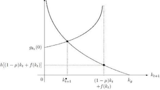
Figure 3. Curves gkt(kt+1)
Properties of g. Parameter kt defines a sheaf of curves. Each of these curves is defined,
continuous and strictly increasing for kt+1Gkt = [0, (1 – )kt + f(kt)] (as u is decreasing). In
the first quadrant, each of these curves has a finite and positive interception with the vertical axis, u[(1 – )kt + f(kt)], and a vertical asymptote given by kt+1 = (1 – )kt + f(kt). When
parameter kt increases, the interception with the vertical axis decreases, the abscissa of the
vertical asymptote increases, and curve () t k
g shifts downward, that is,
) ( > ) (
1 k
g k g
t k t
k if kt < kt+1. (28)
for those k where they are both defined. Hence, curves () t k
g never intersect themselves; they
appear as in Figure 3.
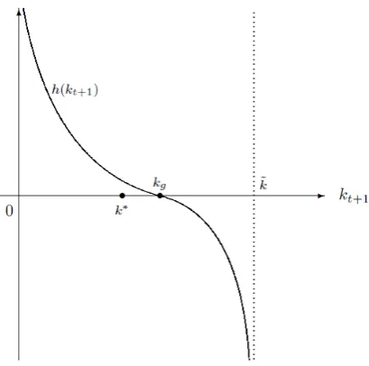
Properties of h. Function h(kt+1) is defined where f(kt+1) – kt+1 > 0, that is, for kt k
~ < <
0 1 ,
19
Figure 4. Curve h(kt+1)
Moreover, = ) )( ( = ] [ ) (0 = ] ) (0 [ ] 0 ) (0 [ = ) ( lim 1 0 1 u f f u k h t kt (29) = ] ) ~ ( )[ ( ] ) ~ ( [ ) (0 = ] ) ~ ( [ ] ~ ) ~ ( [ = ) (
lim~ 1
1 k f k f u k f k k f u k h t k kt
as f(k~) <0 (see Figure 1). Moreover,
0 = 0 ] ) ( [ = ] ) ( [ ] ) ( [ = ) (
g g
g g g g k k f u k f k k f u k
h (30)
0 < ) ( ] ) ( [ ] ) ( [ ] ) ( [ = d d 1 1 1 2 1 1 1 1 t t t t t t t k f k k f u k f k k f u k h
as u<0 and f <0 in 0<kt1 <k~. Curve h(kt+1) appears as in Figure 4.
Lemma 1.Givenkt (0, k*):
1. there exists a unique kt1(0,kˆ) which solves (Wt), where kˆ= min[(1 )kt + f(kt),
kg], that is, there exists a unique kt1 which solves (Wt) on the interval where both
gkt(kt+1) and h(kt+1) are defined and positive;
2. kt 1>kt
20 3. kt 1<k*
.
Proof.
1. Consider equation ( t1)= ( t1) t
k k h k
g on the restricted domain kt1[0,kˆ]. For kt+1 0+ we
have (0 ) (0)= [(1 ) t ( t)]
t k t
k g u k f k
g ; hence
< ) (0 0
t k
g ; (31)
by (29) we have
= ) (0
h . (32)
Hence, by (31) and (32) it follows that
).g (0)<h(0
t
k (33)
Since kt+1 = (1 – )kt + f(kt) is the vertical asymptote of gkt(kt1), we have
. = } )] ( )
{[(1 t t
t
k k f k
g (34)
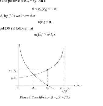
In order to compare gkt and h at the other estreme of the domain, kˆ , three cases must be
distinguished:
(a) If
, < ) ( )
(1 kt f kt kg (35)
then kˆ=(1)kt f(kt) and curves ( t1) t
k k
[image:21.595.168.429.482.629.2]g and h(kt+1) appear as in Figure 5.
21
As kt > 0 and from (35) we have that h(kt+1) is finite and positive at kt+1 = (1 – )kt + f (kt), that
is,
0 < h[(1 – )kt + f (kt)] < (36)
By (34) and (36) it follows that
)].gkt{[(1 )kt f(kt)] }> h[(1 )kt f(kt
(37)
By continuity and thanks to (33) and (37), we conclude that there exists a unique
)), ( )
(1 (0,
1 t t
t k f k
k that is, kt1(0,kˆ)
which satisfies (Wt) (see Figure 5).
(b) If
kg < (1 – )kt + f(kt), (38)
then kˆ=kg and curves gkt(kt1) and h(kt+1) appear as in Figure 6. By (38) we deduce that
) ( t1 t
k k
g is finite and positive at kt+1 = kg, that is
0 < gkt(kg) < + . (39)
On the other hand, by (30) we know that
h(kg) = 0. (30)
Hence, by (39) and (30) it follows that
[image:22.595.150.489.319.670.2]gkt(kg) > h(kg). (40)
22
By continuity and thanks to (33) and (40) we conclude that there exists a unique
), (0,
1 g
t k
k that is, kt1(0,kˆ)
which satisfies (Wt) (see Figure 6).
(c) If
kg = (1 – )kt + f(kt),
then )kˆ=kg =(1)kt f(kt and curves ( t1) t
k k
g and h(kt+1) appear as in Figure 7. In this
case
= } )] ( ) {[(1 )
ˆ
( t t
t k t
k k g k f k
g (41)
and
0.h(kˆ)h(kg)= (42)
Hence by (41) and (42) it follows that
).g (kˆ)>h(kˆ
t
k (43)
By continuity and thanks to (33) and (43) we conclude that there exists a unique
) ˆ (0,
1 k
kt (58)
[image:23.595.179.412.430.605.2]which satisfies (Wt) (see Figure 7).
Figure 7. Case 1(c): kg = (1 – )kt + f(kt)
23
] ) ( [ = ] ) ( ) [(1 = )
( t t t t t t
t
k k u k f k k u f k k
g
] ) ( [ ] ) ( [ = )
(
t t t
t f k
k k f u k h
hence )( t)< ( t t
k k h k
g as [f(kt) ]/ > 1 for kt < k*.
Curves )( t1 t
k k
g and h(kt+1) appear as in Figure 8; hence the solution kt1 of (Wt) must thus
[image:24.595.215.387.188.334.2]lie on the right of kt.
Figure 8. Lemma 1, item 2
3. Draw curves ( t1) t
k k
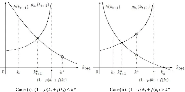
g and h(kt+1) on the same graph (see Figure 9). Two cases must be
distinguished.
(i) If (1 – )kt + f(kt) k*, by item 1 of the this Lemma 1, cases (a) or (c), we deduce that
1
t
k < (1 – )kt + f(kt); hence kt 1<k*
(see Figure 9(i)).
(ii) If (1 – )kt + f(kt) k*, evaluate gkt(kt1) and h(kt+1) at kt+1 = k*:
) * (k g
t
k = u[f(kt) kt (k* kt)]
] ) * ( [ ] * ) * ( [ = ) *
(
k f k k f u k
h = u[f(k*) k*] due to (2).
As kt <k*, then f(kt) kt (k* kt) < f(k*) k*; as u is decreasing, then g (k*)
t
k > h(k*).
Curves )( t1 t
k k
g and h(kt+1) appear thus as in Figure 9(ii); hence the solution kt1 of (Wt)
must thus lie on the left of k*.
24
[image:25.595.116.478.73.253.2]Case (i): (1 – )kt + f(kt) k* Case(ii): (1 – )kt + f(kt) k*
Figure 9. Lemma 1, item 3
Now, we are going to show that if k0 = k*, equation (Wt) defines a constant sequence: kt = k*,
t = 1, 2, 3, ....
Lemma 2Ifkt = k*,there exists a uniquekt 1 k*
which solves (Wt).
Proof. Thanks to equation (2) it is straightforward to verify that equation gk*(kt+1) = h(kt+1) is
satisfied by kt1 k*
. Thus, it is enough to observe that gk*(kt+1) is a monotonically
increasing function of kt+1 while h(kt+1) is a monotonically decreasing function of kt+1 to
conclude that kt1 k* is the unique solution of gk*(kt+1) = h(kt+1). □
Lemmas 1 and 2 entail that, given k0 (0, k*], a sequence {kt}t=1 contained in (0, k*] is
univocally defined by recurrence by equation (Wt).
Lemma 3. k = k* is the unique steady state of sequence {kt}t=1.
Proof. A steady state of {kt}t=1 is a value of k such that kt = kt+1 = k. Substituting it into (Wt),
we obtain:
u[f(k) k (kk) ] = [ ( ) ][ ( ) ]
k f k k f u
which, after simplification, reduces to, [f (k) ]/ = 1, whose unique solution is k = k* (see
25
Proposition. If k0 =k0 < k*, the sequence {kt}t=1 of capital/labour ratios defined by (Wt)
converges monotonically to the steady state k* defined by the Ramsey modified golden rule (2).
Proof. By Lemma 1, if k0 <k* the sequence {kt}t=1 is monotonically increasing (thanks to item 2) and upper bounded by k* (thanks to item 3). Hence it must converge to some k, i.e.,
k kt t
lim . (44)
In order to prove that k = k* observe that, by definition, the elements kt of the sequence satisfy equations (Wt). Consider the limit for t→∞ of (Wt):
] ) ( [ ] ) ( [ lim = )] ( ) ( [
lim 1 1 1
1
t t t t t t t t
t f k
k k f u k k k k f u .
Thanks to the continuity of functions u, f and f we can write
] ) lim ( [ ] lim ) lim ( [ = )] lim lim ( lim ) lim (
[ 1 1 1 1
t t
t t t t t t t t t t t
t f k
k k f u k k k k f u
which, thanks to (44), can be written as
] ) ( [ ] ) ( [ = )] ( ) ( [
f k k k k u f k k f k
u ;
after simplification, this equation in k reduces to [f (k) ]/ = 1, whose unique solution is
k = k* (see equation (2)). This completes the proof. □
Figure 10 displays how {kt}t=1 takes shape as sequence of the abscissas of the interceptions of curves ()
t
k
g with curve h(). As k0 k1 k2 k3 k* and thanks to (28), curves g appear as in the diagram. Moreover, it is easy to verify that curve gk*(k) crosses
curve h(k) at k = k*: in fact, gk*(k*) = u[f(k*) k* (k* k*)] = u[f(k*) k*] and h(k*) = u
26
Figure 10. Sequence {kt}t=1
A simplest proof of the convergence result can be given as follows if we limit to a local
result: calculate the total differential of (Wt) with respect to kt and kt+1:
= } d d 1] )
( ]{[ )
(
[ 1 1
f kt kt kt kt f kt kt kt
u
=1{u[f(kt1)kt1][f(kt1)]2 u[f(kt1)kt1]f (kt1)}dkt1;
evaluate at the steady state, k*, (where f(k*) – = ) and re-arrange; we obtain
, 1
1 = d d
* 1
t t
k k
where
) * ( ) (1
) * ( ) * ( =
u k f u
and * = f(k*) k*. As u > 0, u < 0 and f < 0 then > 0 and
1. < d d < 0
* 1
t t
k k
This proves the local stability of k*: if k0 is taken sufficiently close to k* then it converges to
k* monotonically. The Proposition at page 25 contains a global result.
A remarkable characteristic of the convergence results just seen is that they both have been obtained without assuming any transversality condition, i.e. without the need to anticipate the solution of infinitely many optimization problems. No perfect foresight is thus needed here. For any given level of the capital/labour ratio, kt, the consumer chooses kt+1 just by comparing