The Solution of Optimal Two Impulse Transfer between Elliptical Orbits with Plane Change

(1)

http://www.scirp.org/journal/ijaa ISSN Online: 2161-4725

ISSN Print: 2161-4717

DOI: 10.4236/ijaa.2017.73010 Jul. 20, 2017 125 International Journal of Astronomy and Astrophysics

The Solution of Optimal Two-Impulse Transfer

between Elliptical Orbits with Plane Change

M. H. A. Youssef

Astronomy Department, Faculty of Science, Cairo University, Cairo, Egypt

Abstract

The optimizing total velocity increment ∆v needed for orbital maneuver between two elliptic orbits with plane change is investigated. Two-impulse or-bital transfer is used based on a changing of transfer velocities concept due to the changing in the energy. The transferring has been made between two el-liptic orbits having a common centre of attraction with changing in their planes in standard Hohmann transfer with the terminal orbit which is elliptic orbit and not circular. We develop a treatment based on the elements of ellip-tic orbits a e1, 1, a e2, 2 and a eT, T of the initial orbit, final orbit and trans-ferred orbit respectively. The first impulse ΔV1 at the perigee induces a

rota-tion of the orbital plane by θ1 which will be minimized. The second impulse 2

ΔV at apogee is induced an angle θ2 to product the final elliptic orbit. The

total plane change required α θ θ= +1 2. We calculate the total impulse ∆v

and minimize by optimizing angle of plane’s variation θ1. We obtain a

poly-nomial equation of six degrees on the two transfer angles between neither two elliptic orbits θ1 and θ2= −α θ1. The solution obtained numerically, using

programming code of MATHEMATICA V10, with no condition on the ec-centricity or the semi-major axis of the initial, transformed, and the final or-bits. We find that there are constrains on the transfer angles θ1 and

α

. For

α

it must be between 40˚ and 160˚, and there is no solution if

α

is less than 40˚ and bigger than 160˚ and θ1 takes the values less than 40˚. The

minimum total velocity increments obtained at the value of θ1 less than 25

o

and

α

equal to 160˚. This is an interesting result in orbital transfer problem in which the change of orbital plane is necessary for the transferring.

Keywords

Orbital Mechanics, Astrodynamics, Optimization, Elliptic Hohmann Transfer

How to cite this paper: Youssef, M.H.A. (2017) The Solution of Optimal Two-Impulse Transfer between Elliptical Orbits with Plane Change. International Journal of Astrono-my and Astrophysics, 7, 125-132.

https://doi.org/10.4236/ijaa.2017.73010

Received: April 10, 2017 Accepted: July 17, 2017 Published: July 20, 2017

http://creativecommons.org/licenses/by/4.0/

(2)

DOI: 10.4236/ijaa.2017.73010 126 International Journal of Astronomy and Astrophysics

1. Introduction

The problem of the optimal impulsive transfer between two orbits is almost se-venty years old, but the question, how many impulses are still open despite of the theories and a lot of numerical works developed in this field. In 1925, Hoh-mann produced a numerical study showing that the optimum two-impulse transfer path between coplanar circular orbits is a semi-ellipse, tangential at its apsides to both circular orbits, with an impulse occurring at each apse. Hoh-mann transfer is generalized to the elliptic case (transfer between two coaxial el-liptic orbits). A large number of works have been made to optimize non-coplanar transfer between circular or elliptic orbits having collinear major axes [1][2][3][4]. An analytical solution for optimal two-impulse 180˚ transfer between non-coplanar elliptic orbits and the optimal orientation of the transfer plane is presented with numerical solutions under some terminal conditions in

[5]. A polynomial equation of six degrees on the generalized Hohmann transfer with plane change using energy concepts is obtained without analytical solution

[6]. A fundamental result is presented in Lawden’s work where a primer vector satisfying necessary condition for optimality of the total delta velocity was in-troduced in coplanar transfer [7]. The necessary condition for optimality is re-duced to a polynomial equation of the eighth degrees on the semi-latus rectum and with the fixed transfer angle, for which no solution has been found in two-impulse transfer between two elliptic coplanar orbits [8]. In this work, we give the optimum total velocity increment ∆v required to transfer between two elliptic orbits having a common centre of attraction with plane change. We con-sidered here generalized Hohmann transfer consisted of two impulses through semi-elliptic path. The first thrust ΔV1 occurring at the perigee does not only

produce a transfer ellipse but also induce a rotation of the orbital plane by θ1.

The second impulse ΔV2 at apogee is induced an angle θ2 to produce the

fi-nal elliptic orbit. An engine firing in the out of plane direction is required for the change of the plane. The point of firing becomes a point in the new orbit, and the burn point becomes the intersection of the current orbit and the desired orbit. In the following treatment, we used a changing of transfer velocities concept due to the changing in the energy in terms of the elliptic orbital elements a e1, 1, a e2, 2

and a eT, T2 of the initial orbit, final orbit and transferred orbit respectively. We

calculate the total impulse ∆v and minimize by optimizing angle of plane’s vari-ation θ1, we obtain a polynomial equation of six degrees on the two transfer

an-gles between neither two elliptic orbits θ1 and θ2 with any restrictions on their

eccentricities and semi-major axis, nor any restrictions on the terminal distances and the initial and final orbital velocities. The solution obtained numerically, using programming code of MATHEMATICA V10. The total velocity impulse is mini-mized by optimizing angle of plane’s variation numerically under some constrains of the transfer angles.

2. Formulation and Optimization

(3)

DOI: 10.4236/ijaa.2017.73010 127 International Journal of Astronomy and Astrophysics to another by means of a change in velocity, begins with the energy as

2 2 1

V

r a

µ   = _ − _

  (1)

where V is the magnitude of the orbital velocity at some point, r the

magni-tude of the radius from the focus to that point, a semi major axis of the orbit and

µ

_{the gravitational constant of the attracting body. Equation (1) can be} rear-ranged as

2

2 2

V

r a

µ µ

− = − (2)

where it is evident that

kinetic energy potential energy total energy satellite mass + satellite mass =satellite mass

Note that (energy/satellite mass) is dependent only on a, an increases, energy

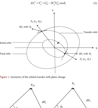
increases. Orbital maneuvers are based on the principle that an orbit is uniquely determined by the position and velocity vector at any point [9]. Conversely, changing the velocity vector at any point instantly transforms the trajectory to a new one corresponding to the new velocity vector. So if we want to move a spacecraft to a higher orbit, we have to increase the semi-major axis (adding energy to the orbit) by increasing velocity. On the other hand, to move the spacecraft to a lower orbit, we decrease the semi-major axis (and the energy) by decreasing the velocity. Any conic orbit can be transformed into another conic orbit by changing the spacecraft velocity vector. Coplanar maneuver only in-volves the change of the orbit without changing the orbit plane, we have four kind of coplanar maneuvers (i) Tangential orbit Maneuver, (ii) Non-tangential orbit Maneuver, (iii) Hohmann transfer, (iv) Bi-elliptic orbit transfer. The Hohmann’s transfer is the minimum two-impulse transfer between coplanar circular or elliptic, it can be used to transfer a satellite between two noninter-secting orbits, coaxial, aligned. The fundamental of the Hohmann’s transfer is a simple maneuver. This maneuver employs an intermediate elliptic orbit which is tangent to both initial and final orbits at their apsides. A ∆V maneuver (refers to the difference between the initial and final velocity vectors),can raise or lower the perigee or apogee, a change in inclination, escape, reduction or increase in period, begin a 2+ maneuver sequence of burns. This process takes two steps, to get from orbit one to the transfer orbit, we change the orbit’s energy by changing the spacecraft’s velocity by an amount ∆V1. Then when the spacecraft gets to

orbit two, we must change its energy again by changing its velocity by an amount ∆V2, if we don’t the spacecraft will remain in the transfer orbit,

indefi-nitely, returning to where it started in orbit one, then back to orbit two, etc. Thus, the complete maneuver requires two separate energy changes, accom-plished by changing the orbital velocities (using ∆V1 and∆V2). For mission

(4)

DOI: 10.4236/ijaa.2017.73010 128 International Journal of Astronomy and Astrophysics low orbit to a higher orbit or vice versa with different planes, to do this, it had to increase velocity twice, ∆V1 and ∆V2. At the point P r1

(

1,θ1

)

, we apply an

impulse with magnitude ∆V1 increase the spacecraft’s velocity, taking the

spacecraft out of orbit one and putting it into the transfer orbit, the transfer orbit crosses the final orbit at the point P r2

(

2,θ2

)

, where we apply an impulse with

magnitude ∆V2 putting it into the final orbit as in Figure 1. At point P r1

(

1,θ1

)

, 1

r is the perigee distance of orbit one (The initial orbit with an elements a1, e1)

and r1=a1

(

1−e1

)

and at the point P r2

(

2,θ2

)

, r2 is the apogee distance of

orbit two (The final orbit with an elements a2, e2) and r2=a2

(

1−e2

)

. The

transfer orbit given by an elements aT and eT, where

2 1 2 1

T r r e

r r

− =

+ (3)

1 2

2

T

a a

a = + (4)

The total velocity increment will obtain from the following relations, as seen in Figure 2.

2 2 2 2 2

1 p TP

2

p TP

cos

1

V

V V

θ

[image:4.595.208.542.309.678.2]

∆

=

+

−

₍₅₎

Figure 1. Geometry of the orbital transfer with plane change.

(5)

(

)

2 2 2 2 2

2 A TA

2

p TA

cos

1

V

V V

α θ

∆

=

+

−

(6)

where Vp, VTP, VA, and VTA are the perigee velocity at P1 of the initial orbit,

the transfer’s velocity of the transfer orbit at perigee, the apogee velocity at P2

of the final orbit and the transfer’s velocity of the transfer orbit at apogee respec-tively.

(

)

(

1

)

1 1 1 1 p e V a e µ + = − ;

(

)

(

)

1 1 T TP T T e V a e µ + = −

(

)

(

2

)

2 2 1 1 A e V a e µ − = + ;

(

)

(

)

1 1 T TA T T e V a e µ − = + 1

[image:5.595.206.543.110.718.2]

θ _and θ₂_{are the angles between the velocities at} P₁ and P2 as shown in Figure 1, and θ2= −α θ1. So Equations ((5) and (6)) will be

(

)

(

1

)

(

)

(

1

)

(

)

1 1

1 1 1 1

2 cos

1 1 1 1

T T

T T T T

e e e e

V

a e a e a e a e

µ

θ

    + + + + ∆ + − _ _{ } _ − − __ − _{ }_ − _ =

 

(7)

(

)

(

2

)

(

)

(

2

)

(

)

(

)

2 1

2 2 2 2

1 1 1 1

2 cos

1 1 1 1

T T

T T T T

e e e e

V

a e a e a e a e

µ

α θ

   

− − − −

∆ + − _ _{ } _ −

+ + __ + _{ }_{ } + __

= ₍₈₎

Thus, the total increment of the velocity is

1 2

V V V

∆ = ∆ + ∆

₍₉₎

For simplicity let

(

)

(

1

)

1 1 1 1 e A a e µ + = − ,

(

)

(

)

1 1 T T T e B a e µ + = − ,

(

)

(

2

)

2 2 1 1 e C a e µ − = + ,

(

)

(

)

1 1 T T T e D a e µ − = + (10) Then (9) will be in the form

( )

1

( ) (

1

)

2 cos 2 cos

V A B AB

θ

 C D CD

α θ



∆ = _ + − _+ _ + − − _ (11)

1

θ _{to be optimized by the condition of minimization}

1 Δ 0. V θ ∂ = ∂

By partial differentiation of (11) with respect to θ1 and equating to zero, and

after arrangements and clearing fraction, we find that

( )

(

)

2 2 1 1 1 1 sin sin

2 cos 2 cos

CD AB

A B AB C D CD

α θ θ

θ α θ

− =

+ − + − − (12)

From which we can deduce that

( )

(

)

(

)

( )

(

)

2 2

2 2 2 2 2

2 1 1

2 2 1

AB C D CD bx a x x

CD A B AB x a b x b abx x

 _{+ −} ₊ ₋  ₋         = _ + − _{ }_ − + − − __ (13) where 1 cos

x= θ , 1−x2 =sin

θ

₁,

a

=

sin

α

,

b

=

cos

α

(14)

(6)

(

)

(

)

(

)

(

)

(

)

(

)

(

)

(

)

(

)

2 2

2 2 2

2 2 3

2 2

1 2 2 4 2

AB C D CD A B b CD ABb bAB CD x

AB C D CD A B a b x

bAB CD CD AB a b x

x aAB CD abCD A B x abCD AB aAB CD x

+ − + +   −_ + + + _   +_ + − − − _ − − + + = _ − _ Let

(

)

(

)

2

1

AB C

+

D

−

CD A B b

+

=

E

2

2 2CD ABb −2bAB CD=E

(

)

(

)

(

2 2

)

3

–_AB C+D +CD A B a+ – b _=E

(

2 2

)

4

2bAB CD+2CD AB a −b =E

5 2aAB CD=E

(

)

6

– 2abCD A+B =E

7 4abCD AB−2aAB CD=E

Then

(

)

2 3 2 2

1 2 3 4 1 5 6 7

E +E x+E x +E x = −x E +E x+E x

(15)

After squaring and some reduction, we may write

(

)

(

)

(

)

(

)

(

)

(

)

(

)

2 2 2 2 2 2

1 5 1 2 5 6 1 3 2 5 7 6 5

3 2 2 2 4

1 4 2 3 6 7 5 6 2 4 3 7 5 7 6

5 2 2 6

3 4 6 7 4 7

2 2 2 2

2 2 2 2 2 2

2 2 0

E E E E E E x E E E E E E E x

E E E E E E E E x E E E E E E E x

E E E E x E E x

− + − + + − − − + + − + + − + + + + − + + = (16) Set 2 2

1 5 0

E −E =F

1 2 5 6 1

2E E −2E E =F

2 2 2

1 3 2 5 7 6 5 2

2E E +E −2E E −E −E =F

1 4 2 3 6 7 5 6 3

2E E +2E E −2E E +2E E =F

2 2 2

2 4 3 7 5 7 6 4

2E E +E −E +2E E +E =F

3 4 6 7 5

2E E +2E E =F

2 2

4 7 6

E −E =F

Then Equation (16) will be an algebraic equation of degree six in θ1 (with

α

explicitly) in the form

2 3 4 5 6

0 1 2 3 4 5 6 0

F +F x+F x +F x +F x +F x +F x = (17)

3. Solution and Discussion

(7)

DOI: 10.4236/ijaa.2017.73010 131 International Journal of Astronomy and Astrophysics the computed values of the velocities at perigee and apogee, and the transfer an-gle θ1. The necessary optimal conditions are obtained using analytical code and

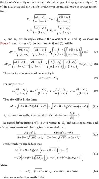
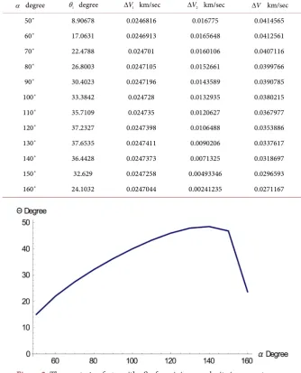
different numerical code by MATHEMATICA V10. For each value of eccentrici-ties, and semi-majors, we find at least one root satisfied Equation (17). Also we find that there is constrains on the transfer angles θ1 and

α

as seen in Table 1 and Figure 3. For

α

it must be between 40˚ and 160˚, there is no solution if

α

is less than 40˚ and bigger than 160˚. Also the minimum total velocity in-crements will obtain with the value of θ1 less than 40˚ and

α

less than 160˚.

This is an interesting result in orbital transfer problem in which the change of orbital plane is necessary for the transferring.

4. Conclusion

[image:7.595.204.539.297.708.2]

We give a complete analytical analysis and numerical solution of optimal two-

Table 1. The values of α and θ1 which satisfying the solution and the optimal velocity.

α degree θ1 degree ∆V1 km/sec ∆V2 km/sec ∆V km/sec

50˚ 8.90678 0.0246816 0.016775 0.0414565

60˚ 17.0631 0.0246913 0.0165648 0.0412561

70˚ 22.4788 0.024701 0.0160106 0.0407116

80˚ 26.8003 0.0247105 0.0152661 0.0399766

90˚ 30.4023 0.0247196 0.0143589 0.0390785

100˚ 33.3842 0.024728 0.0132935 0.0380215

110˚ 35.7109 0.024735 0.0120627 0.0367977

120˚ 37.2327 0.0247398 0.0106488 0.0353886 130˚ 37.6535 0.0247411 0.0090206 0.0337617 140˚ 36.4428 0.0247373 0.0071325 0.0318697 150˚ 32.629 0.0247258 0.00493346 0.0296593 160˚ 24.1032 0.0247044 0.00241235 0.0271167

[image:7.595.204.539.300.714.2]

(8)

DOI: 10.4236/ijaa.2017.73010 132 International Journal of Astronomy and Astrophysics impulse transfer with plane change. Our treatment is based on a changing of transfer velocities concept due to the changing in the energy. We obtained the total velocity increment ∆ =∆ + ∆V V1 V2 of the two impulses ∆V1 and ∆V2

at perigee and apogee respectively, in terms of the semi-major axes a a a1, 2, T and the eccentricities e e e1, 2, T of the initial orbit, final orbit and transferred or-bit respectively. The transferring has been made between two elliptic oror-bits hav-ing a common centre of attraction with changhav-ing in their planes in a tight Hoh-mann’s transfer with the terminal orbit which is elliptic orbit. We minimized

v

∆ _{by optimizing angle of plane’s variation} θ₁_{. We obtain a polynomial}

equa-tion of six degrees on the two transfer angles between neither two elliptic orbits

1

θ _and θ₂= −α θ₁_{. The optimization process here depends on the value of the}

plane change with no constrain on a or e, the optimal maneuver can be purely propulsive. It is shown that whenever an impulse is applied, a plane change is made. The necessary conditions for the optimal split of the plane changes are derived and simulated in computer program for the solution. We optimized with new constrains in the angles of transfer, for

α

it must be between 40˚ and 160˚ and there is no solution if

α

is less than 40˚ and bigger than 160o_,

1

θ _takes

the values less than 40˚. The minimum total velocity increments obtained at the value of θ1 less than 25˚ and

α

equal to 160˚. This constrains are newer and

more different than which are obtained in others works [3][4][5]. This is an in-teresting result in orbital transfer problem in which the change of orbital plane is necessary for the transferring.

References

[1] Roth, H. (1967) Minimization of the Velocity Increment for a Bi-Elliptic Transfer with Plane Change. Astronautica Acta, 13, 119-130.

[2] Eckel, K. (1962) Optimize Non-Coplanar Transfers between Circular Orbits. Astro- nautica Acta, 8, 177.

[3] Hiller, H. (1966) Optimum Impulsive Transfers between Non-Coplanar Elliptic Or-bits Having Collinear Major Axes. Planetary and Space Science, 14, 773-789.

https://doi.org/10.1016/0032-0633(66)90106-1

[4] Hiller, H. (1965) Optimum Transfers between Non-Coplanar Circular Orbits. Pla-netary and Space Science, 13, 147-161.

https://doi.org/10.1016/0032-0633(65)90184-4

[5] Sun, F.T. (1969) Analytic Solution for Optimal Two-Impulse 180˚_{Transfer between}

Noncoplanar Orbits and the Optimal Orientation of the Transfer Plane. AIAA Journal, 7, 1898-1904. https://doi.org/10.2514/3.5478

[6] Kamel, M. and Soliman, S. (2011) On the Generalized Hohmann Transfer with Plane Change Using Energy Concepts. MME, 15, 183-191.

[7] Lawden, D. (1991) Optimal Transfer between Coplanar Elliptical Orbits. Guidance and Control, 15, 3.

[8] Altman, S.P. and Pistiner, J.S. (1963) Minimum Velocity Increment Solution for Two-Impulse Coplanar Orbital Transfer. AIAA Journal, 1, 435-442.

https://doi.org/10.2514/3.1551

(9)

Submit or recommend next manuscript to SCIRP and we will provide best service for you:

Accepting pre-submission inquiries through Email, Facebook, LinkedIn, Twitter, etc. A wide selection of journals (inclusive of 9 subjects, more than 200 journals)

Providing 24-hour high-quality service User-friendly online submission system Fair and swift peer-review system

Efficient typesetting and proofreading procedure

Display of the result of downloads and visits, as well as the number of cited articles Maximum dissemination of your research work

Submit your manuscript at: http://papersubmission.scirp.org/