Munich Personal RePEc Archive
Absorptive Capacity and Innovative
Capability: An Approach to Estimation
Polterovich, Victor and Tonis, Alexander
Central Economics and Mathematics Institute RAS, Moscow, New
Economic School, Moscow
25 June 2014
Online at
https://mpra.ub.uni-muenchen.de/56855/
Absorptive Capacity and Innovative Capability:
An Approach to Estimation
Victor Polterovich and Alexander Tonis
CEMI, RAS, and NES, Moscow
Abstract
The concepts of absorptive capacity and innovative capability have been introduced to
describe abilities of a country to imitate and, accordingly, to create more advanced technologies.
In this paper we suggest new indicators of these two abilities. To calculate them, we develop an
endogenous growth model and an estimation procedure that combines both calibration and
econometric approaches.
The choice of parameters is based on WDI, ICRG and Barro–Lee statistical data for the
period of 1981-2005. As a result, the model generates trajectories of 63 countries and, for most
of them, gives qualitatively correct pictures of their evolution dependently on their initial states
as well as on their absorptive capacity and innovative capability indicators. In particular, club
convergence is demonstrated. The calculations affirm our hypotheses about shapes of absorptive
capacity and innovative capability dependence on the relative productivity level, human capital,
institutional quality and some other factors.
Keywords: imitation, innovation, catching-up development, foreign direct investment, human
capital, equilibrium, evolution of countries distribution
JEL: O33, O41, O43, O57
1. Introduction
Each developing country tries to catch up with the developed world. Unfortunately, only few
economies were able to reach this purpose during last sixty years. Well known Gershenkon’s
argument – “advantage of backwardness” – does not work properly in most cases
(Gershenkon (1962)). Though imitations of technologies and governance methods are much
cheaper than innovations, the imitation process is also costly and requires sophisticated
Different abilities of countries to imitate and to innovate are reflected in the concepts of
absorptive capacity and innovative capability.
The concept of absorptive capacity has been originally introduced as a characteristic of a
firm, namely its "ability to recognize the value of new, external information, assimilate it, and
apply it to commercial ends" (Cohen, Levinthal, 1990). Later on, this concept was applied to a
country as a whole. The imitation process is understood in a broad sense including a choice of
technology (or a method of governance), an acquisition of the rights to use it, its adaptation to
the conditions of the recipient’s country, its modification and, possibly, some improvements.
L. Suarez-Villa was probably the first one who has used (in 1990) a concept of
innovative capability (see http://www.innovativecapacity.com). In Furman, Porter, Stern
(2002, p.1), it is defined as “the ability of a country – as both a political and economic entity – to
produce and commercialize a flow of innovative technology over the long term».
Modeling of imitation and innovation processes constitute the core of modern theories of
endogenous economic growth (Barro and Sala-I-Martin, 1995; Aghion, Howitt, 1998;
Acemogly, Aghion, Zilibotti, 2002a,b). It is widely believed that absorptive capacity is a main
determinant of successful catching-up development.
However, to the best of our knowledge, up to now there is neither general strict
definitions of the absorptive capacity and innovative capability nor convincing methodology to
measure them.
There are a number of papers that try to find main determinants of economic growth (see
Barro (1991), and again Barro and Sala-I-Martin (1995), Aghion and Howitt (1998) for surveys).
However, different factors play different roles at different stages of development. Successful
catching-up is possible only if appropriate policies are implemented at each stage and switching
from one policy to another one is made in time (Acemoglu, Aghion, Zilibotty (2002 a),
Polterovich, Popov ( 2006a,b), Unido (2005)).
Possibilities to arrange good policies depend on our knowledge of absorptive capacity
and innovative capability as well as on factors which influence both quantities. However, the
task to separate and measure two abilities is not trivial. Instead, a number of researches try to
suggest indicators that characterize technological capabilities of countries. In Archibugi , Coco
(2005), authors describe and compare five indicators developed by The World Economic Forum
(WEF), the UN Development Program (UNDP), the UN Industrial Development Organisation
(UNIDO), and the RAND Corporation, and then they suggest their own measure of technological
capability, ArCo. All these indicators are based on a set of country characteristics and,
unfortunately, on “arbitrary weighting schemes with limited theoretical or empirical bases”
For example the index of innovation capability is published by the United Nations
Conference on Trade and Development (UNCTAD) and consists of an unweighted average of an
index of human capital (a weighted average of tertiary and secondary school enrollment rates
and the literacy rate) and a technological activity index (an unweighted average of three per
capita indicators: R&D personnel, U.S. patents granted, and scientific publications).
Rank correlations between indicators are high enough (not less than 0.85) though for
some countries big divergence is observed. For example, Israel ranks 3rd by ArCo, but it ranks 7th by RAND, 21st according to WEF, and 18th according to UNDP (Archibugi , Coco (2005),
p. 186).
In UNIDO (2005), weights were chosen through factor analysis that was carried out on
29 indicators, and five principal factors were labeled as knowledge, inward openness, financial
system, governance, and the political system. The first factor correlates highly with R&D and
innovation, scientific publications, information and communications technology infrastructure,
production certifications and education. Inward openness means imports and inward FDI.
Financial system composite indicator reflects market capitalization, country risk and access to
credit. Then, these factors as well as nine geographical, cultural and natural resource indicators
were taken as regressors for growth rate. The sample included data on 135 countries for two
three years periods: 1992-1994 and 2000-2002. Only financial system, governance, knowledge
and/or their increments were found to be significant.
A similar methodology has been used in World Bank (2008). As much as 34 variables
were used over the 1990–2006 period. To calculate overall index of technological absorptive
capacity four types of characteristics were taken into account: Macroeconomic environment
(general government balance, CPI inflation rate, real exchange rate volatility); Financial
structure and intermediation (liquid liabilities, private credit, financial system deposits); Human
capital (primary educational attainment, percent of population aged 15 and secondary
educational attainment percent of population aged 15; tertiary educational attainment percent of
population aged 15); Governance (Voice and accountability, Political stability, Government
effectiveness, Regulatory quality; Rule of law).
What are the problems these indicators may help to solve? The answer is not quite clear.
Nevertheless Archibugi and Coco write : “Both policy analysts and academic researchers need
new and improved measures of technological capabilities on the performance of nations to
understand economic and social transformations. With regard to policy analysis, this has
relevance for public and business practitioners. Governments constantly require information
about the performance of their own country, and this is often better understood in comparison to
The short survey above demonstrates that, up to now, there are neither general strict
definitions of absorptive capacity and innovative capability nor convincing methodology to
measure them. This paper tries to fill in this gap.
In this paper we try to build indicators that could not only serve for comparisons of
different countries technology levels but also could help to choose most efficient direction to
invest.
Having in mind this goal we introduce the following definitions.
The absorptive capacity of an economy is defined as the cost of 1% increase of its TFP
through technology transfer from other economies.
Analogously, the innovative capability of an economy is defined as the cost of 1%
increase of its TFP through technology innovation.
In both definitions, the cost may be measured as percentage of GDP or capital of a
country.
In this paper, the latter measure is used.
In these definitions, technology is understood in a broad sense as a method of
production, trade, governance, etc.
In what follows we will also use the terms adaptive and innovative abilities, having in
mind that the less is absorptive capacity of a country the larger is its adaptive ability; similarly,
the less is innovative capability of a country the larger its innovative ability.
Different kinds of policies and institutions are required to increase adaptive or innovative
abilities. If for example adaptive ability of a country is much larger than its innovative ability
then it is reasonable to invest into imitation projects. Thus, it is important to measure both
abilities.
Basing on many empirical and theoretical researches one might put forward the following six
hypotheses about dependencies of absorptive capacity and innovative capability on different
factors.
1) Absorptive capacity is negatively connected with relative level of development; the higher
is this level the larger is innovative capability.
The level of development is defined as a ratio of the country productivity parameter to the
productivity of the most advanced economy. A similar assumption is used in Acemoglu, Aghion
and Zilibotti (2002a), where the costs per unit of the productivity increase are taken to be
constant for imitation and linear for innovation. In what follows we assume (and then check),
that the imitation cost function increases and the innovation cost function decreases when the
Barro and Sala-I-Martin (1995). The reason is that less advanced economies may borrow
well-known and cheap technologies that may be obsolete for advanced economies.
The shape of dependence of innovation cost on development levels is more questionable. On
one hand, decreasing rate of return might take place. On the other hand, accelerating effects of
the technical progress occur. We will show that innovation costs are less for most advanced
economies (see also Polterovich, Tonis (2005)).
2) International trade positively influences absorptive capacity.
Import and export both are channels through which new knowledge penetrates into a country.
Import is a source of more advanced equipment. Export orientation is an incentive and an
opportunity to apply new technologies and to study new marketing approaches.
However, there are evidences that the influence of international trade policy on growth
depends on institutional quality and stage of development (Rodríguez, Rodrik (2000),
Polterovich, Popov (2006а,b)). In any case, it is not clear to what extent international trade
volumes are connected with innovative capabilities.
3) Human capital has positive impact on innovative capability. The influence of human capital
on absorptive capacity is much less pronounced since imitation requires less creative workforce.
This is particularly underlined in Acemoglu, Aghion, Zilibotti (2002a), Vandenbussche,
Aghion, Meghir (2004), Rogers (2004). The role of human capital for development was studied
in many earlier papers ( see Lucas (1988), Mankiw, Romer, Weil (1992), Nonneman, Vanhoudt
(1996) and more references in Aghion, Howitt (1998)). However some researchers cast doubt on
significance of human capital, measured as share of education cost in GDP or as literacy rate, for
economic growth (see Levine, Renelt (1992) and polemics in Sala-I-Martin (1997)).
4) Institutional quality positively influences both absorptive capacities and innovative
capabilities.
One may expect, however, that absorptive capacity is much more sensitive to this factor than
innovative capability: innovations start to play substantial role at higher levels of development
when institutional quality is strong enough so that its additional enhancing does not give any
substantial effect.
5) Foreign direct investment may be an effective channel of enhancing absorptive capacity.
However, they may be harmful as well if institutional quality is low and regulation is not rational
enough (Kinoshita Y. (2008)).
6) Banking system is more important for imitation whereas financial markets play decisive role
for innovative development.
This is a conclusion from a number of researches (see Chakraborty, Ra (2006), Deidda,
In what follows we try to check these hypotheses.
To be reliable, the measurement method has to be based on a model which is able to
reproduce a general picture of world economic development. We use data sets for 63 countries
and the time period 1980-2006, and find that this picture is complicated enough. Advanced
economies seem to be converging to each other. Another converging group includes a number of
Latin American and some other countries with 15-30% of the USA GDP per capita. These two
groups seem to be growing with almost equal rates whereas most of African countries fall
behind. It looks like world income is moving toward a distribution with two peaks. This
observation, made by Quah (1993), gave birth to a number of research about ”club
convergence”.
Some explanations of this phenomenon may be got in framework of underdevelopment or
poverty trap theories. There are four different classes of development trap models that consider
the trap as a result of a lack of physical capital, human capital, productivity, and low quality of
economic and political institutions (see Azariadis and Drazen (1990) and Feyrer (2003) for a
survey and references).
Easterly, Levine (2001), and Feyrer (2003) found, however, that factor accumulation can not
explain two peaks distribution: “the output per capita is tending toward twin peaks despite the
tendency toward convergence in the accumulable factors. The productivity residual, on the other
hand, shows movement similar to the distribution of per capita output...” (Feyrer (2003), p.31).
Thus, interactions between innovation and imitation processes and institutional development
should play dominant roles in modeling of the club convergence behavior.
The interactions were studied in a number of papers (see Segerstrom (1991), Barro and
Sala-I-Martin (1995), Aghion , Howitt(1998), Henkin, Polterovich (1999) for surveys, and also
Acemoglu, Aghion, and Zilibotti (2002), Howitt and Mayer-Foulkes (2002), Polterovich, Tonis
(2003, 2005)).
In this paper we consider two modifications of the model developed in Polterovich, Tonis
(2003, 2005) . This model has a number of attractive features that make it a good instrument of
measuring adaptive capacities and innovative capabilities.
a). It is not assumed, as it is done in many other papers, that a country always imitates the most
advanced technology. Every developing country experiences a lot of failures connected with
attempts of borrowing the most recent achievements of the developed world. A rational policy
admits borrowing not only best achievements but experience of many other countries as well
(compare Aghion, Howitt (1998, Chapter 12)).
b). The model takes into account a difference between global and local innovations. The first
c). The model takes into account that the larger is an innovation or an imitation project, the less
probable is its success (in accordance with Howitt and Mayer-Foulkes, 2002). Therefore, both
policies exhibit decreasing rate of return, and the tradeoff between innovation and imitation may
result in producing both of them.
d). In accordance to our model, costs of imitation and innovation in a country may depend not
only on its relative level of development but also on a number of exogenous parameters. This
gives a possibility to study dependence of adaptive capacity and innovative capabilities on broad
variety of parameters.
e). In most investigations, steady states are studied only. However, to generate a picture that
reproduces a real set of countries trajectories, one has to consider transition paths. To do that, we
were forced to simplify our model drastically. The model is quasi-static and generates
trajectories as sequences of static equilibria. The model makes use of many other simplifications
as well.
It was shown that, under stationary exogenous conditions, three types of stable steady states
are possible, where only imitation, only innovation or a mixed policy prevails.
It turned out that the model indeed generates a picture qualitatively similar to the real one.
Roughly speaking, three groups of countries behave differently. There is a tendency to converge
within each group. Countries with low institutional quality have stable underdevelopment traps
near the imitation area. Increase in the quality moves the steady state toward a better position and
turns into a new stable steady state where local innovations and imitations are jointly used.
Under further institutional improvements, a combined imitation-innovation underdevelopment
trap disappears. All countries with high quality of institutions are moving toward the area where
pure innovation policy prevails (see Polterovich and Tonis (2005) where a model with no human
capital is considered).
Below, we use this model to demonstrate how adaptive capacity and innovative capability
can be calculated. Our method combines calibration and econometric approach. In the
calculation process we find how adaptive ability and innovative capability depend on a broad set
of indicators such as level of development, investment risk, international trade, human capital,
availability of physical capital, and some others. Two key values and a few other parameters are
chosen to reproduce trajectories of more than 60 countries from 1980 to 2006. This methodology
permits to check, at least partially, hypothesis a)-e).
Our calculations are based on assumptions about the relationship between royalty receipts and
royalty payments of a country, on the one hand, and innovation and imitation costs on the other
We also suggest a modification of the model where a dynamic equation for human capital is
introduced. It is shown that our main conclusions are stable with respect to variations of the
model.
The plan of the paper is as follows. А static model is described in the next section. In Section
3 we study comparative statics of the model. Section 4 contains the descriptions of a dynamic
model. Data description, the methodology of calibrations and main results are presented in
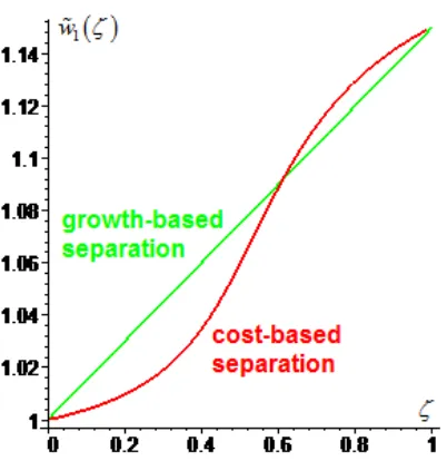
Sections 5-7. Two approaches to calibration are presented. The first one (sections 5-7) is based
on growth-based separation hypothesis: ratio of rates of growth induced by innovations and
imitations is proportional to royalty receipts over royalty payments. In Section 8, an alternative,
cost-based separation hypothesis is used: the ratio of royalty receipts to royalty payments is
proportional to the ratio of innovation to imitation costs. The results of absorptive capacity and
innovative capability calculations are presented and discussed in Section 9. Section 10
concludes.
2. A static model
This model is a modification of a model from Acemoglu, Aghion, Zilibotti (2002a).
There are three kinds of goods in our economy: final good, capital and the continuum set of
high-technology intermediate goods indexed by ν∈ [0, 1].
Every period, final good is competitively produced from the intermediate goods. Each
intermediate good ν is characterized by its productivity Aν . The production function for the final
good is given by
1
0
( , )
Y =
∫
F NAν Xν dν, (1)where N is the number of workers (so, NA
ν is the “effective labor”), Xν is the quantity of
intermediate good ν involved in the production process, and F is homogeneous of degree 1:
F NA X( ν, ν)=NA f xν ( )ν (2)
where x X
NA
ν ν
ν
= , x ν is the “normalized” quantity of intermediate good. Here we assume that f
satisfies Inada conditions and xf′′(x) + f′(x) falls from ∞ to 0, as x proceeds from 0 to ∞.
Throughout this paper, a special case of Cobb — Douglas production function will be
considered:
1
( , ) ( )
F NA X NA α X α
ν ν ν ν
−
= ⋅ , 0<α <1.
We suppose that final good can be sold at price 1. The price of intermediate good ν is pν . A
producer of final good chooses its demand for each of intermediate goods,Xν, taking all prices
as given, so as to maximize its profit:
1
0
max X Y p X d
ν ν ν ν
−
∫
→ (3)From the optimality conditions, one gets the following inverse demand function:
f xʹ′( )ν = pν. (4)
Intermediate goods can be produced from capital. The production function in the intermediate
goods sector is assumed to be linear: one unit of capital can be converted to one unit of
intermediate good1.
In each sector ν ∈ [0, 1], only one firm enjoys the full access to the technology of producing the
corresponding intermediate good, so the market for each intermediate good is monopolistic. Let
the rental price of capital be r. Then firm’s profit Vν is given by
(
)
( ) '( )
Vν = pν −r Xν =NAν f xν −r xν. (5)
The firm is facing the demand of the final good sector for its product and monopolistically
chooses pν so as to maximize its profitVν.
In each sector ν , the monopolist firm lives for one period of time. At the beginning of the
period, each sector starts with the same (country-specific) physical capital K, human capital H
and productivity levelA. This level represents the cumulative technological knowledge achieved
by the economy up to that date. Prior to producing its intermediate good, a firm may spend a part
of its future profit and a part of its physical capital to perform technological innovations and
imitations, thus raising its productivity fromA toAν. Afterwards, it produces input with higher
productivityAν.
It is easy to check that in the case of Cobb – Douglas production function, maximization
of (5) entails
2 1 ( ) ( ) ( )
r x f xʹ′ fʹ′ʹ′ x x α xα−
= + = , (6)
and
( )
V e x NA
ν = ν, (7)
1
We can use one-to one production function because the unit of intermediate good ν along with the technological parameter Aν can be properly adjusted.
where
2
( ) ( ) (1 )
e x =−x fʹ′ʹ′ x =α −α xα.
As follows from the above formulas, under Cobb – Douglas production function GDP is
given by
1 ( )
Y = NAx%α = NA%−αKα (8)
where 1
0
A A d
ν ν
=
∫
% is the average productivity level over all producers of intermediate product
and K is the total amount of capital used in the intermediate product sector. Note that due to (8),
A% is closely related to the total factor productivity (TFP) of the economy: the growth rate of TFP
is (1 – α) times the growth rate of A%. The same can be said about the initial productivity level A.
Now let us describe the evolution of the productivity variable (and, hence, TFP). The
considerations above concern the domestic economy. There are also foreign countries, in which
initial productivity levels may differ from domestic one. Denote by A an initial productivity
level of the most developed economy. Along with the domestic absolute productivity level A, let
us consider the relative level a A A
= which measures the distance to the world technology
frontier. It represents the position of the domestic technologies among other ones.
As we mentioned above, each firm performs imitation and/or innovation prior to production.
Let b1 and 2
b denote, respectively, the sizes of imitation and innovation projects. Each project
may result in one of two outcomes, success or failure. If the imitation (innovation) was
successful, firm’s productivity rises at growth rate b1 ( 2
b ); otherwise, it remains the same. If
both projects were successful, the productivity turns out to be (1+b1)(1+b2) times higher. Thus,
after both actions, the technology parameterAν is given by
Aν =(1+ξ1)(1+ξ2)A, (9)
where ξ1 (ξ2) is a random variable equal to b1 ( 2
b ) in the case of successful imitation
(innovation) of firm ν, and 0 otherwise. This multiplicative function brings about a
complementarity effect of imitation and innovation: a progress in imitation results in greater
marginal productivity of innovation, and vice versa.
We postulate that probabilities of imitation and innovation success are given by the
functions ψi( ), bi i=1, 2:
( ) i , 1, 2 i i
i i
b i
b µ ψ
µ
= =
whereb1 ( )b2 is a size imitation (innovation) project and
1 ( 2)
µ µ is a positive parameter.
Naturally, larger project is more risky. The expected value of the productivity growth rate as a
“proper” result of a project bi is equal to ψi( )b bi i; µi may be interpreted as the expectation of
the result of an infinitely large project .
Firms cannot imitate technologies which have not been developed anywhere in the world, so
the size of the imitation project is subject to constraint
1 b1 1 a
+ ≤ , (10)
where a A
A
= . This constraint takes into account that a firm can imitate not only the most
advanced technology but also an “intermediate” one.
Now let us introduce the costs of imitation and innovation. Technological development
includes not only invention or adoption of new methods of production, but also implementation
of these methods to the existent machinery. To adopt the costs of spreading technological
knowledge over the economy, we assume that the costs of imitation and innovation depend not
only on the size of the corresponding projectbi, but also on the amount of capital to be upgraded.
Specifically, in order to undertake projectbi, the firm has to invest Kq bi i units of capital, where
K is the average capital stock over the economy (equal to the capital stock of a representative
firm).
It is assumed that q1 and q2, the per-unit costs of imitation and innovation, depend on the
relative average productivity level of our economy (that is “a distance to the world technology
frontier”) at the beginning of the period, and on the accumulated stock of human capital H:
( , )
i i
q =q a H , qi are continuous and differentiable. We assume also (and this is supported by
empirical evidences) that q1 is increasing and q2 is decreasing in a. According to this
assumption, it gets more difficult to imitate and easier to innovate as the domestic technology
gets closer to the world technology frontier. Indeed, for less developed countries, it may be
reasonable to imitate not very advanced technology which are cheaper to buy (some of them are
not protected by intellectual property laws at all) and simpler to implement using experience
accumulated by other countries. The innovation process is likely to exhibit some economy of
scale due to a positive externality exerted by the stock of accumulated knowledge, so more
advance countries incur less costs.
Evidently, human capital accumulation decreases the innovation costs. This is not so obvious
follows, we assume for simplicity that imitation cost, q1 does not depend on human capital. This
assumption will be checked below.
Generally, q1 and q2 may depend on some other country-specific parameters as well. In the
empirical section, we consider qi as functions of savings rates and indicators of institutional
quality.
Both forms of technological development are modeled in a similar way here. However, the
opportunities for imitation and innovation change in different directions as a increases. In
particular, when a is close to 1, there is almost nothing to imitate. This is taken into account by
constraint (10).
Under the above assumptions, the expected profit of the firm ν (net of technology investment
expenditures) is given by
E(Πν)=E V( )ν −rZ=E V( )ν −rK q a b
(
1( ) 1+q a H b2( , ν) 2)
, (11)where V
ν is given by (5), the expectation is taken over the four possible realizations of
success/failure of innovation/imitation. Hν is the amount of human capital used by firm ν , and
Z is the total expected amount of physical capital invested in innovation and imitation:
Z=K q a b
(
1( ) 1+q a H b2( , ν) 2)
. (12)In the beginning of each period, the firm chooses b1 and 2
b to maximize its expected net profit
(11). We assume that Hν does not depend on ν: Hν= H for all ν .
In what follows we assume that firms’ demand for human capital is satisfied, and do not
take into account the costs of physical capital involved in human capital increase.
Denote
1 2 1 1 2 2
( , ) ( ) ( ), ( )i i (1 i( ) ), i i 1, 2
w b b =w b w b w b = +ψ b b i= , (13)
and let k K
NA
= – per capita capital stock over the initial productivity.
Then, taken into account (7), (9), (10), (11) and (13), the firm maximization problem may
be written as follows.
(
1 2 1 1 2 2)
( ) ( ) ( , ) ( ) ( ( ) ( , ) ) max
E Πν =NA e x w b b −r x k q a b +q a H b → , (14)
1 1
0≤b ≤b, b2 ≥0, (15)
where b1 1 1
a
= − .
2
2 1
( ) ( ) (1 ) 1
1 , 0
( ) ( ) ( )
e x x f x x
x x
r x f x xf x x
α
α
α α
η η
α − α
ʹ′ʹ′ − ⎛ ⎞
=− = =⎜ − ⎟ = >
ʹ′ + ʹ′ʹ′ ⎝ ⎠ , (16)
where η=1 /α−1. Therefore, (14) is equivalent to the following problem:
1 2 1 1 2 2
( , ) [ ( ) ( , ) ] max xw b b k q a b q a H b
η − + → . (17)
In accordance to (17), and (9), a firm, having capital K and human capital H in a state a,
spends Z = (K q a b1
( )
1+q a H b2(
,)
2) , chooses b1, b2, and demands Xν =NA xν capital units. Inequilibrium, one has to get
K =X +Z , or k =xw b b( , )1 2 +k q a b[ ( )1 1+q a H b2( , ) ]2 , (18)
where
1
0
X X d
ν ν
=
∫
, k KNA
= .
An equilibrium is defined as a triple x b b, ,1 2 such that the pair
1 2
( ,b b ) is a solution of (17), (15)
under givenx, and equality (18) holds.
We assume that the equilibrium exists and is unique.
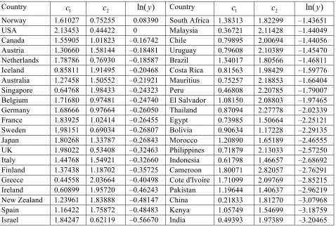
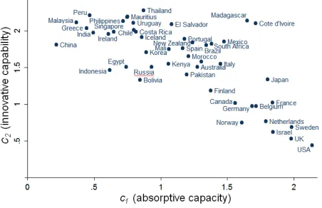
In the framework of the model described above, absorptive capacity and innovative capability
may be calculated as c1= q1b1 , c2= q2b2 where projects b1, b2 each gives 1% increase of TFP
of a capital unit. This means b1ψ1( b1)=0.01(1 – α)–1 , b2ψ2( b2)=0.01(1 – α) –1. Therefore,
ci 0.01(1 α)−1µiqi / (µi 0.01(1 α) ),−1 i 1, 2
= − − − = . (19)
Formula (19) will be used to measure the absorptive capacity and innovative capability of
countries.
3. Analysis of the static model
Let us denote
(
)
2
2 ( )
( ) i i ( ) ( ) = i , 1, 2
i i i i i i i
i i i
dw b
b b b b i
db b
µ
ϕ ψ ψ
µ ʹ′
= = + =
+ , (20)
and write down the first order conditions for the problem (17), (15).
ηx w b⋅ 2( ) ( )2 ϕ1 b1 ≤kq a1( ), (21)
1 1 2 2 2
ηx w b⋅ ( )ϕ ( )b ≤kq a H( , ), (22)
If an inequality holds in (21)-(22) then a related variable 0 i
b = or H H
ν = .
( )
(
)
(
)
(
)
1 2 1 1 2 2 2 2 1 1 1 1 1 2 2 2
( , ) Z = k , ( ) ( ) ( ) ( ) )
z b b q a b q a H b w b b b w b b b
NAx x
ν
ν ν
η ϕ ϕ
= + = + (23)
do not depend on x ,H
ν ν. Therefore, the balance condition (18) takes the form
( ) ( )
( ) ( )
i i i i
i i
i i i i
b b b
R b
w b S b
ϕ
= = , k x
(
w b b( , )1 2 z b b( , )1 2)
ν= + , (24)
where Si(bi)=wi(bi)/ϕi(bi).
The following system of equations follows from (21) – (22), (24) and determines an interior
equilibrium.
1 1 1 1 2 2 2
1
1 1 1 1 1 2 2
( ) ( ) ( )
1
( ) ( ) ( ) ( )
w b w b b b
b
q a b b w b
ϕ
ηϕ ϕ
= + + , (25)
2 2 2 2 1 1 1
2
2 2 2 2 2 1 1
( ) ( ) ( )
1
( , ) ( ) ( ) ( )
w b w b b b
b
q a H b b w b
ϕ
ηϕ ϕ
= + + , (26)
Let us define:
1
1 1 Q ( )
( ) a
q a = , 2
2 1 ( , )
( , ) Q a H
q a H
= ,
(27)
2
( ) ( )( )
( ) , 1, 2
( )
i i i i i i i i
i i
i i i
w b b b b
S b i
b
µ µ µ
ϕ µ
+ + +
= = = , ( ) ( ) / ( )
( ) i i i
i i i i i i i
b b
R b b S b
w b ϕ
= = . (28)
Then one gets from (25), (26)
1 1 1 2 2 1
Q ( )a =S b( )[1/η+R b( )]+b, (29)
2 2 2 1 1 2
Q ( ,a H ) S ( )[1/b R b( )] b
ν = η+ + . (30)
Assume that bi are not too large so that Ri are increasing functions. Then right-hand sides of (29), (30)
both are increasing in each bi; Q1 is decreasing in a; Q2 is increasing in both variables. Differentiating
(29), (30), it is easy to check that b a H1( , ), is decreasing ina,
2( , )
b a H is increasing ina, and both
functions are increasing in H.
Thus, we have proved the following statement:
Consider the interior solution case, and let b1, b2 be not too large for some a. Then there exists a
This comparative statics result is analogous to Proposition 1 in Pikulina (2009), where firms
rationally choose the amount of human capital.
4. Dynamic model
We consider a quasi-dynamic model that generates trajectories by iterations of the static
model described above. Thus it is assumed that firms have one period horizon, and that all of
them get the average (expected) technologyA% that were found at a previous period but partially
depreciated2. Therefore,
A+1=(1−ρ)A%, A+1=(1−ρ)A% (31)
where 1 1 1 1 2 2 2
0 (1 ( ) )(1 ( ) )
A A d b b b b A
ν ν ψ ψ
=
∫
= + +% and ρ is the knowledge depreciation rate
(0 ≤ρ≤ 1).
Assume that output Y of the final good producers is taxed to finance education sector. Let
( )a
τ be the education tax rate depending on a. It is simple to check (see formulas (3)-(5), (11))
that this tax does not influence the choice of projects b1 , b2 so that equations (25), (26) hold.
We assume that the evolution of human capital His subject to the following equation:
1 1 (1 H) ( ) ( )
N H δ NH m a τ a Y
+ + = − + , (32)
where δHis the human capital depreciation rate (0 ≤δH≤ 1), m a( ) is a multiplier measuring the
impact of education on human capital.
Here A+1 , H+1 play the same role for the next-period firms as A, H for the current-period
firms. In each period, all firms start from the same initial productivity and human capital due to
assumed total spillovers of technology and human capital among sectors. The assumptions about
one period horizon as well as about independence of industry’s future productivity level on its
current innovation/imitation efforts seem to be very restrictive. In particular, the model does not
describe the behavior of long-run investors. To eliminate these shortcomings, one could use an
OLG model. In this case, however, it would be difficult to investigate transition dynamics rather
than steady states.
To finish with the description of the model, we need to specify, how labor and capital evolve
over time. We assume that the number of workers N grows at a constant rate
N g :
N+1 =(1+gN)N,
where Nand 1 N
+ denote the number of workers, respectively, in the current and the next period.
2
Let K and K+1 be the capital stocks at the current period and the next one, respectively. We
assume that the next-period capital stock is determined by the following equation
1 (1 K) (1 ( )) K δ K σ τ a Y
+ = − + − (33)
where δK∈[0,1] is the capital depreciation rate, Y is the total output of the final good, and
[0,1]
σ∈ is a (constant) saving rate. Parameter σ is assumed to be country-specific. It may
depend on the quality of institutions and investment climate in the country. We also assume that
ρ <δK , i. e. physical capital depreciates faster than technology.
A dynamic equilibrium in the model is defined as a sequence of variables {Kt , At , xt , Ht , b1t ,
b2t}t such that, in each period t, four quantities x H bt, t, 1t,b2t form a static equilibrium under
1 t K
− , At−1, Ht−1, and evolution equations (31)-(33) hold.
To summarize, the economy evolves as follows. At the beginning of the period, all firms in a
country start from the same productivity level A. Firms choose the sizes of their imitation and
innovation projects which maximize their profits. Then random events are realized; success or
failure of these projects and, correspondingly, random values Aν turn out to be known.
Production takes place and profits are revealed. The next-period productivity level, human and
physical capital stocks are determined. All next-period firms start their projects from the new
productivity level. They make their innovations and imitations determining their successors’
productivity level, and so on.
Assume that the productivity of the most developed countryA increases with a constant
growth rateg . Then
(
)
(
)
1 1 1 1 2 1 ( , )1
w b b A A
a
A g A
ρ + + + − = =
+ or
1 2 1
( , ) w b b
a a
γ
+ = , (34)
where 1
1 g γ ρ + = − .
Equation (33) takes the following form:
(
)
1 1
1 1 1 2
(1 ) (1 ( )) (1 ) 1 ( , )
K
N
K K a Y
k
N A g w b b A
δ σ τ
ρ + + + + − + − = =
+ − , or 1
(
)
1 2(1 ( )) ( ) (1 ) (1 ) 1 ( , )
K
N
a f x k
k
g w b b
σ τ δ
ρ +
− + −
=
+ − . (35)
In addition to the model described above, another, simplified version of the model will be
considered. The only difference of the simplified model from the original one is that the
evolution of H is given exogenously rather than determined by (32); in this case, τ( )a is
supposed to be zero. This model is equivalent to the model presented in Polterovich and Tonis
(2005). The two versions of the model will be referred to as the model with, respectively,
A stationary equilibrium for the model with exogenous human capital is defined as a dynamic
one at which variables k and a are not changing over time (and exogenous human capital H is
also stationary). As follows from (34) and (35), equations for a stationary equilibrium take the
form
1 2 ( , )
w b b =γ , (34’)
(
)
1 2(1 ( )) ( )
(1 N) 1 ( , ) (1 K)
a f x k
g w b b
σ τ
ρ δ
−
=
+ − − − . (35’)
1 2 1 2
( , ) ( , )
k x
w b b z b b
=
+ (24’)
1 1 1 1 2 2 2
1
1 1 1 1 1 2 2
( ) ( ) ( )
1
( ) ( ) ( ) ( )
w b w b b b
b
q a b b w b
ϕ
ηϕ ϕ
= + + , (25’)
2 2 2 2 1 1 1
2
2 2 2 2 2 1 1
( ) ( ) ( )
1
( , ) ( ) ( ) ( )
w b w b b b
b
q a H b b w b
ϕ
ηϕ ϕ
= + + , (26’)
An important question is whether a given stationary equilibrium is stable or not. If it is stable,
then convergence takes place within the corresponding group of countries. Otherwise, the
equilibrium marks the boundary between the attraction areas of different centers of convergence.
Stability conditions for stationary equilibria under exogenous human capital are established in
Polterovich and Tonis (2005).
Proposition (Polterovich and Tonis, 2005). Consider a stationary equilibrium, at which
1 1
b <b. Then
1. If there is no innovation in equilibrium, then the equilibrium is asymptotically stable.
2. If there is no imitation in equilibrium, then the equilibrium is unstable.
3. If both imitation and innovation are present in the equilibrium, then its stability is
depends on the relation between the absolute values of q1 a
∂
∂ and 2
q a
∂
∂ : if 2 1 / / q a q a −∂ ∂ ∂ ∂
is high, then the stationary equilibrium is unstable; otherwise, it is stable.
A stable stationary equilibrium may be considered as prediction of long-run development of
the economy. In some cases, there could be multiple stable stationary equilibria.
Country-specific exogenous parameters affecting the normalized cost functions (institutional quality,
international trade and so on) thereby influence possible stable stationary equilibria – not only
their position but even their structure: steady states may emerge or vanish. Even if the
equilibrium structure does not change, the long-run outcome may change substantially. For
close to the upper boundary of this area, a short-run positive shock of exogenous parameters may
get it out of the trap.
Note that under endogenous human capital, there is no natural concept of stationary
equilibrium, because equation (32) suggests that h H A
= is to be stationary over time, so that
1 2
( ) ( ) ( , ) ( ) (1 N)(1 A) (1 H)
m a a w b b f x h
g g
τ
δ =
+ + − − , (32’)
whereas according to (26’), b2 depends on H rather than on h. There could be a stationary
equilibrium, if b2 were depending on h. Note also that when we calibrate the model, a proper
interpretation of human capital is needed: what H (or h) is? If human capital is measured in
schooling years, as in Barro – Lee dataset used here, then it cannot grow exponentially as H
does in a stationary equilibrium. Not only the duration but also the quality of education should be
taken into account, if we want to calibrate stationary regimes.
5. Calibration of the model: data and methodology
Sections 5–9 give an empirical adjustment of the model considered above. We are going to test
some of basic assumptions of the model (in particular, those concerning the per-unit cost
functions of innovation and imitation) and to adjust the parameters of the model to the statistical
data. Our approach to empirical investigation combines two methods: estimation of a linear
regression model (calculating TFP and estimating the normalized cost functions for imitation and
innovation) and non-linear optimization procedure used for calibration of “basic” parameters of
the model.
One of the most important questions concerning calibration of the model is how to calculate
proxies for q1 and q2, the normalized costs of imitation and innovation. Saying this by a
different way, we have to separate TFP growth effects of imitation and innovation. As follows
from the previous section (see (25) and (26)), q1 and q2 can be calculated, if we know which
part of the growth rate can be explained by imitation and which one by innovation. Obtaining
this information from regular cross-country data is a non-trivial problem. We suggest using the
ratio of royalty receipts over royalty payments to deal with it (with bought licenses being a proxy
for the result of imitation and sold ones for innovation). We suggest also two alternative ways to
separate imitation-based and innovation-based growth. One way called “growth-based
Another way entails such separation that the ratio of imitation costs to innovation costs is
proportional to the royalty-receipts-payments ratio.
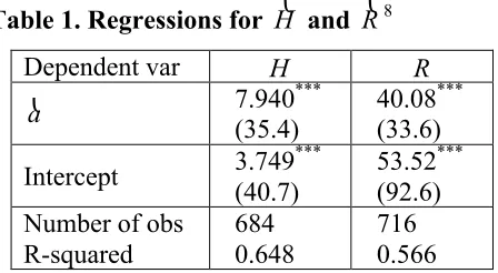
The estimation process consists of a preliminary stage and an iteration cycle. At the
preliminary stage, TFP is calculated using basic national account data (GDP, population, capital,
investment) and initial values of basic parameters are set. Then a cyclical routine starts. Given
the basic parameters and the data on royalty receipts and royalty payments q1 and q2 are
calculated. Then the normalized cost functions are estimated using regressions with q1 and q2 as
dependent variables and a number of explanatory variables. After the set of regression
coefficients is derived, the dynamic model of Section 4 (or similar) is run with the estimated cost
functions. The predictive quality of the dynamic model is used as a criterion based on which the
basic parameters are corrected and a new loop starts until the error of prediction becomes close
to minimum. A more detailed description of the algorithm will be given later on.
We use data from the following sources: World Development Indicators (WDI, 2008),
International Country Risk Guide (ICRG, 2004), physical capital stock dataset (Nehru and
Dhareshwar, 1993), Barro-Lee dataset on human capital. The data structure is as follows:
Y – GDP, years 1980,…, 2006, 180 countries; source: WDI;
N – population, years 1980,…, 2006, 188 countries; source: WDI;
I – gross fixed capital formation, years 1980,…, 2006, 173 countries; source: WDI;
K – capital stock, years 1980,…,1990, 89 countries; source: Nehru and Dhareshwar;
R – ICRG composite risk index, measure of the institutional quality, years 1984,…, 2003,
129 countries; source: ICRG; R∈
[
0,100]
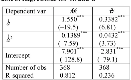
; R is higher for lower risks;B
L – royalty payments, total value of licenses bought, years 1980,…, 2006, 123 countries;
source: WDI;
S
L – royalty receipts, total value of licenses sold, years 1980,…, 2006, 88 countries;
source: WDI;
T – manufactures trade (export+import) , years 1980,…, 2006, 164 countries; source: WDI;
B – domestic credit provided by banking sector, years 1980,…, 2006, 180 countries;
source: WDI;
F – foreign direct investment, years 1980,…, 2006, 172 countries; source: WDI;
H – total years of schooling (age 15+), measure of human capital stock, years 1980,…, 2000,
111 countries; source: Barro-Lee dataset.
ED – public spendings on education, years 1990-2006, 105 countries; source: WDI;
Using WDI data on GDP, all these variables (except for N, R, P and H) are put to the same
unit of measure, namely, constant 2005 international $ (adjusted to PPP).
In order to smooth fluctuations, we have averaged the data by 9 three-year periods
(1980-1982,…,2004-2006). The time subscript refers to the median year of the corresponding
three-year period: for example, Y1981 for period 1980-1982 and so on.
Using the above data, we are going to calibrate our dynamic model, i. e. estimate its
parameters so as to obtain good quality of prediction. We consider two versions of our model: a
simplified one where human capital is considered as an exogenous parameter and a full version
with endogenous human capital, as in Section 4.
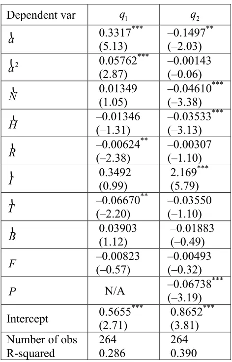
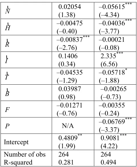
We assume also that the per-unit cost functions of innovation and imitation q1 and q2 depend
not only on a but also on country-specific variables N ,H, R, I , T, B, F and P. We are
going to estimate these functions parametrically: we assume that they are quasi-polynomial
functions determined by an array of coefficients β which is to be estimated. The specific form
of the cost functions and their coefficients β will be defined later on.
So, the calibration of the model involves estimating the following parameters:
α – the parameter of the Cobb-Douglas production function;
1
µ – maximal growth rate due to imitation;
2
µ – maximal growth rate due to innovation;
ρ – technology obsolescence rate;
λ – adjustment ratio used for estimating the share of innovation and imitation in TFP growth
(see below);
β – a set of regression coefficients of two cost functions q1 and q2 (with dependent variables
listed above: relative level of development, population, human capital etc). Coefficients β are
found using the OLS method.
Parameters µ1, µ2, ρ and λ are called “basic” and are estimated using a non-linear
To obtain plausible results, we need to suggest estimators for the above parameters so as to
reproduce the actual growth dynamics in various countries. To measure the level of country’s
development, we use its relative per capita GDP y which can be defined as the ratio of country’s
per capita GDP to that of the USA:
/
/ USA USA
Y N y
Y N
=
We start from y1981, the relative per capita GDP in 1981 (corresponding to the earliest period
1980-1982 in our data series) and, using the dynamic model, try to predict y2005, the relative per
capita GDP in 2005 (corresponding to the latest period 2004-2006). There are many possible
ways to measure the quality of prediction. Here we use the minimal sum of squares criterion: the
sum of squares of logarithmic errors
(
)
22005 2005 ˆ
ln( ) ln( )
E=
∑
y − yshould be minimized, where y2005 and yˆ2005 are, respectively, the actual and the predicted
relative per capita GDP values.
The problem of minimizing E as a function of the parameters is difficult because of its large
dimension. To simplify the problem, we decompose it into three stages. At the first, preliminary
stage, we estimate α , the parameter of the Cobb-Douglas production function, from the standard growth regression and calculate the productivity variable. The second and the third stage are
repeated cyclically. At the second stage, we fix the basic parameters µ1, µ2, ρ, λ and
calculate q1, q2 using LB,LS and the basic parameters. Then we estimate β as the set of
coefficients in two regressions with dependent variables q1 and q2 and explanatory variables a,
N,H, R, I , T, B, F , P (so β is a function of the basic parameters). At the third stage, all
these data are put into the dynamic model and it is iterated starting from y1981 and predicting
2005
y . Here the basic parameters are given; coefficients β are determined at the second stage;
variables N, R, I, T, B, F, P (and H in the case of exogenous human capital) are taken
from the statistical data; a (and H in the case of endogenous human capital) is calculated for
the previous 3-year period (for 1981 – taken from the data). Then the second and the third stages
are repeated for slightly perturbed values of the basic parameters in order to calculate the
parameters. Then basic parameters are changed in the direction opposite to the gradient and the
procedure returns to the second stage. Thereby, the basic parameters µ1, µ2, ρ and λ are
calibrated through minimization of E.
Such decomposition of the calibration problem not only simplifies the process of calibration
but also allows estimation of statistical significance of factors contributing to the absorptive
capacity and innovative capability. A seeming disadvantage of this method is that its result is not
an exact solution to the calibration problem because at the first stage, not E but other function is
minimized (actually, the sum of squares of errors in regression for each of qi is minimized). In
fact, we restrict our opportunities for adjustment getting in return for an opportunity to interpret
key results at intermediate stages, and, in the case of success, to get higher confidence that the
success is not occasional.
Now we are going to describe the procedure in more detail. Let us start with a description of
the first stage. We need to decompose the per capita GDP growth rate into three components:
growth due to capital accumulation, innovation and imitation. Firstly, we need to extract the
growth rate of the total factor productivity from the annual per capita GDP growth rate. In period
1984,1987, , 2005
t= K , the latter is given by
1/3
3 3
/
1 /
t t t
t t Y N g
Y− N−
⎛ ⎞
=⎜ ⎟ −
⎝ ⎠
.
Due to our assumption about the Cobb-Douglas form of the production function, GDP can be
represented as follows (see (8)):
( )
1Y = NA%−α Xα,
where X is the amount of capital used in production and A% is the average productivity level
proportional to the TFP. Denote by gX the growth rate of X
N , the per capita value of the
intermediate good, and by gK, the growth rate of K
N the capita stock per capita. According to
the model, X is equal to the total capital stock K less the imitation and innovation expenditures
which constitute a small share of K. So, gK could be a good proxy for gX. Hence, as follows
from the standard growth accounting considerations, α can be estimated from the following
ln(1+g)=αln(1+gK) const+ (36)
We have found systematic cross-country data on capital stock only for the period until 1990. For
more recent years, we have to apply the perpetual inventory estimation3 method using the recursive formula of capital stock evolution:
1 (1 )
t K t t
K δ K I
+ = − + ,
where δK, the rate of physical capital depreciation, is estimated from the capital stock data
before 1990. The estimated levels of δ for different countries vary from 2% to 7%, with average 4.13% per year4.
It can be seen from the data that the expenditures on imitation and innovation (R&D and
royalties) constitute a small part of GDP, typically, less than 2%, so we can put X =K for
simplicity. Thus, to extract the productivity, we use the following formula:
1 1
Y A
K
α α
−
⎛ ⎞
=⎜ ⎟
⎝ ⎠
% ,
where α can be found from regression (36). In our computations, the estimate for α is close
to 0.50.
Based on A%, we construct some other country-specific variables useful for our analysis:
USA
A a
A
=
% %
% – relative productivity level (compared to that of the USA), a measure for the distance
to the frontier;
ln( )
a(= a%;
3 1
(1 )
t t
t
A w
A ρ
+
=
−
% %
% – a proxy for productivity growth factor w in the model (actually, w%=w,
when the productivity growth in the current period is equal to that in the next one).
3
This method is used in a number of papers on growth accounting (e. g., see Bosworth and Collins, 2003 or Senhadji, 2000).
4
Now let us turn to the second stage, the estimation of q1 and q2, using the WDI data on
royalties5. Firstly, we need to separate the imitation and innovation components of the productivity growth factor w% based on the values of bought and sold licenses. As it has been
already said, we use two alternative ways of separation: growth-based and cost-based. Under
growth-based separation, the following heuristic formula is used:
2 1 ( 1 1) S B L w w L λ − = −
% % . (38)
This is an important hypothesis: ratio of TFP rates of growth induced by innovations and
imitations is proportional to royalty receipts over royalty payments. We have no
microfoundations behind this hypothesis. Implicitly, it describes a mechanism by which
domestic knowledge, embodied into royalty receipts, and foreign knowledge, embodied into
royalty payments, both influence domestic rate of growth.
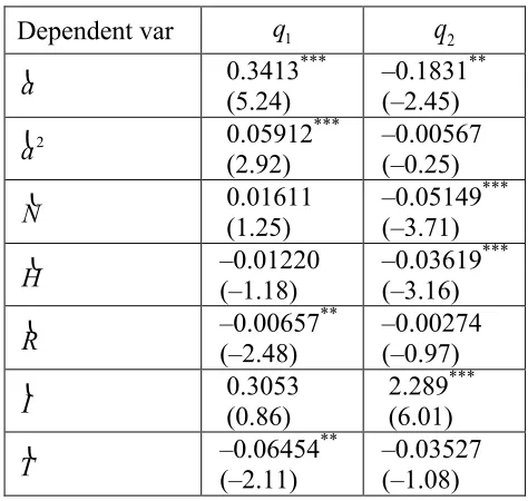
In Section 8, an alternative method of determining contributions of imitation and innovation
will be presented. We call it cost-based separation. Under cost-based separation, the ratio of
royalty receipts to royalty payments is proportional to the ratio of innovation to imitation costs
rather than growth rates.
Since wi = +1 biψ( )bi
% %
% , one gets
( 1) 1 i i i i i w b w µ µ − = + − % % %,
where bi
%are proxies for
i b.
If a country is so close to the world technology frontier that the size of the imitation project b%1
exceeds the feasible level (that for which the imitated technology does exist), then b%1 and 2 b% are
recalculated so as to satisfy this requirement (see (13)).
Now from the first-order conditions for the firm’s optimal choice of b1 and
2
b , we obtain 1 q%
and q%2 which are proxies for 1
q and q2:
2 1 2 1 1 1 w q b η µ = ⎛ ⎞ + ⎜ ⎟ ⎝ ⎠ % % % ; 1 2 2 2 2 1 w q b η µ = ⎛ ⎞ + ⎜ ⎟ ⎝ ⎠ % %
% . (39)
5