Forecasting Value at Risk and Expected Shortfall using Fractionally Integrated Models of Conditional Volatility: International Evidence

(1)

Munich Personal RePEc Archive

Forecasting Value-at-Risk and Expected

Shortfall using Fractionally Integrated

Models of Conditional Volatility:

International Evidence

Degiannakis, Stavros and Floros, Christos and Dent, Pamela

Department of Economics, Portsmouth Business School, University

of Portsmouth, Postgraduate Department of Business

Administration, Hellenic Open University

2013

(2)

Forecasting Value-at-Risk and Expected Shortfall using Fractionally Integrated Models of Conditional Volatility: International Evidence

Stavros Degiannakis1,2,∞, Christos Floros1 and Pamela Dent1

1_{Department of Economics, Portsmouth Business School, University of Portsmouth,}

Richmond Building, Portland Street, Portsmouth, UK, PO1 3DE

2

Postgraduate Department of Business Administration, Hellenic Open University, Aristotelous 18, Greece, 26 335

Abstract

The present study compares the performance of the long memory FIGARCH model, with that of the short memory GARCH specification, in the forecasting of multi-period Value-at-Risk (VaR) and Expected Shortfall (ES) across 20 stock indices worldwide. The dataset is comprised of daily data covering the period from 1989 to 2009. The research addresses the question of whether or not accounting for long memory in the conditional variance specification improves the accuracy of the VaR and ES forecasts produced, particularly for longer time horizons. Accounting for fractional integration in the conditional variance model does not appear to improve the accuracy of the VaR forecasts for the 1-day-ahead, 10-day-ahead and 20-day-ahead forecasting horizons relative to the short memory GARCH specification. Additionally, the results suggest that underestimation of the true VaR figure becomes less prevalent as the forecasting horizon increases. Furthermore, the GARCH model has a lower quadratic loss between actual returns and ES forecasts, for the majority of the indices considered for the 10-day and 20-day forecasting horizons. Therefore, a long memory volatility model compared to a short memory GARCH model does not appear to improve the VaR and ES forecasting accuracy, even for longer forecasting horizons. Finally, the rolling-sampled estimated FIGARCH parameters change less smoothly over time compared to the GARCH models. Hence, the parameters' time-variant characteristic cannot be entirely due to the news information arrival process of the market; a portion must be due to the FIGARCH modelling process itself.

Keywords: Expected Shortfall, Long Memory, Multi-period Forecasting, Value-at-Risk,

Volatility Forecasting.

JEL Classifications: G17; G15; C15; C32; C53.

(3)

1. Introduction – Motivation and Review of Literature

The recent financial crisis has emphasised the importance for financial institutions of producing reliable Value-at-Risk (VaR) and Expected Shortfall (ES) forecasts. VaR quantifies the maximum amount of loss for a portfolio of assets, under normal market conditions over a given period of time and at a certain confidence level. ES quantifies the expected value of the loss, given that a VaR violation has occurred.

Following the recommendations of the Basel Committee on Banking Supervision (1996, 2006), many financial institutions have flexibility over their choice of model for estimating VaR. The guidelines prescribe, however, that financial institutions should use up to one year of data to calculate the VaR of their portfolios for a ten-day holding period1. The Basel Committee recommend producing multi-step VaR forecasts by scaling up the daily VaR figure using the square root of time rule2. However, this method is criticised in the literature, with Engle (2004) noting that it makes the invalid assumption that volatilities over time are constant. Further, Rossignolo et al. (2011) give emphasis to both the current (Basel II3) and proposed regulations (Basel III4) with regard to VaR estimation. Focusing on 1-trading-day VaR, they compare results from current and proposed regulations and suggest that heavy-tailed distributions are the most accurate technique to model market risks.

The majority of existing models for forecasting VaR and ES are focused on producing accurate forecasts for 1-trading-day. An enormous variety of VaR models have been tested in the literature, including both parametric and non-parametric models. The results have not been entirely consistent, often suggesting that the optimum choice of model, as well as the distributional assumptions, may depend upon a number of factors including the market for which the model is being estimated, the length and frequency of the data series, and whether or not the VaR relates to long or short trading positions (Angelidis et al., 2004; Shao et al., 2009).

1_{Following the financial crash, amendments to the regulations were announced, necessitating financial}

institutions to calculate a ‘stressed value-at-risk’ measure, using data covering a year of trading in which the financial institution incurred significant losses (Basel Committee on Banking Supervision, 2009).

2_{To account for the non-linear price characteristics of option contracts, financial institutions are expected to}

move towards calculating a full 10-day VaR for positions involving such contracts.

3_{Basel II VaR quantitative requirements include: (a) daily-basis estimation; (b) confidence level set at 99%; (c)} one-year minimum sample extension with quarterly or more frequent updates; (d) no specific models prescribed: banks are free to adopt their own schemes; (e) regular backtesting and stress testing programme for validation purposes, see Rossignolo et al. (2011).

(4)

The Generalised Autoregressive Conditionally Heteroskedastic (GARCH) model has been shown in the literature to produce reasonable low and high frequency VaR forecasts across a variety of markets and under different distributional assumptions. For example Sriananthakumar and Silvapulle (2003) estimate the VaR for daily returns and select the simple GARCH(1,1) model with Student-t errors as the preferred model. Some studies have concluded that the use of a skewed, rather than a symmetrical, distribution for the standardised residuals produces superior VaR forecasts. For example, Giot and Laurent (2003, 2004) find the skewed Student-t APARCH model to be superior to other specifications for estimating both in-sample and out-of-sample VaR. On the other hand, Angelidis and Degiannakis (2007) conclude that the Student-t and skewed Student-t overestimate the true VaR, and consequently other distributions such as the normal may be more appropriate for the standardised residuals. There is some debate over the relative merits of conditional volatility models compared to other specifications. Whilst, Danielsson and Morimoto (2000) find that conditional volatility models produce more volatile VaR predictions, Kuester et al. (2006) conclude that the VaR violations arising from unconditional VaR models do not occur independently throughout the estimation period, but may be clustered together.

Accounting for long memory and asymmetries in the conditional volatility process has been shown to improve VaR and ES forecasting accuracy for short (1-day and 5-day) forecasting horizons (Härdle and Mungo, 2008; Angelidis and Degiannakis, 2007).

Recently, Halbleib and Pohlmeimer (2012) propose a methodology of computing VaR based on the principle of optimal combination that accurately predicts losses during periods of high financial risk. They develop data-driven VaR approaches that provide robust VaR forecasts; the examined methods include the ARMA-GARCH, RiskMetricsTM and ARMA-FIGARCH. They argue that popular VaR methods perform very differently from calm to crisis periods. Further, they show that, in the case of 1-day VaR forecasts, proper distributional assumptions (Student-t with estimated degrees of freedom, skewed Student-t

and extreme value theory), deliver better quantile estimates and VaR forecasts.

(5)

inherently flawed". Further, they show that the EGARCH technique brings no significant advantage over the GARCH method for daily time horizon.

Finally, Chen and Lu (2010) review the robustness and accuracy of several VaR estimation methods, under normal, Student-t and normal inverse Gaussian (NIG) distributional assumptions, and further test both the unconditional and conditional coverage properties of all the models using the Christoffersen's test, the Ljung-Box test and the dynamic quantile test. Using data from Dow Jones Industrial, DAX 30 and Singapore STI, they argue that conditional autoregressive VaR (CAViaR) and the NIG-based estimation are robust and deliver accurate VaR estimation for the 1-day forecasting interval, whilst the filtered historical simulation (FHS) and filtered EVT perform well for 5-day forecasting interval5.

The aim of this paper is to test empirically whether the short memory GARCH model is outperformed for forecasting multi-period VaR for longer time horizons (10-day and 20-day) by the long memory FIGARCH model, which accounts for the persistence of financial volatility (Baillie et al., 1996; Bollerslev and Mikkelsen, 1996; Nagayasu, 2008)6.

The FIGARCH specification has been shown in some empirical studies to produce superior VaR forecasts (Caporin, 2008; Tang and Shieh, 2006). However, these contrast with the findings of McMillan and Kambouroudis (2009) who conclude that the FIGARCH (as well as the RiskMetricsTM and HYGARCH) specifications are adequate to forecast the volatility of smaller emerging markets at a 5% significance, but that the APARCH model is superior for modelling a 99% VaR.

Recently, attention has turned towards extending the existing literature on the accuracy of various modelling specifications to produce one-step-ahead VaR forecasts, to formulate reliable modelling techniques for multi-step-ahead VaR forecasts. For example, historical simulation using past data on the sensitivity of the assets within a portfolio to macroeconomic factors has been used to estimate 1-day and 10-day VaR (Semenov, 2009). Furthermore, a Monte Carlo simulation has been shown to produce useful estimates of intra-day VaR using tick-by-tick data (Dionne et al., 2009; Brooks and Persand, 2003).

The empirical analysis in this paper makes use of an adaptation of the Monte Carlo simulation technique of Christoffersen (2003) for estimating multiple-step-ahead VaR and ES forecasts to the FIGARCH model. This enables comparisons to be made between the

5_{Chen and Lu (2010) show that NIG works well if the market is normal, whereas the method provides low} accurate VaR values within a financial crisis period.

6_{It should be recognised that some authors suggest that accounting for structural breaks in volatility (Granger}

(6)

forecasting performances of the GARCH and FIGARCH models for i) 1-step-ahead, ii) 10-step-ahead and iii) 20-10-step-ahead VaR and ES predictions. The 95% VaR and 95% ES forecasting performances of the GARCH and FIGARCH models are tested on daily data across 20 leading stock indices worldwide.

This study further provides evidence for the time-variant characteristic of the estimated parameters7. In particular, this paper contributes to the debate on the out-of-sample forecast performance of fractionally integrated models (see Ellis and Wilson, 2004). The out-of-sample forecast performance of the GARCH and FIGARCH models is investigated in order to examine (i) whether the FIGARCH model provides superior multi-period VaR and ES forecasts and (ii) in what extend do the rolling-sampled estimated parameters confirm a time-variant characteristic (see Degiannakis et al., 2008).

We show that i) the long memory FIGARCH model, as compared to the short memory GARCH model, does not appear to improve the VaR and ES forecasting accuracy and ii) the estimated parameters of the models present a time-varying characteristic, which can be linked to market dynamics in response to the unexpected news. However, the estimated parameters of the FIGARCH model exhibit relatively a more time-varying characteristic than those of the GARCH model, inferring evidence that not all of the time-varying characteristics can be due to the news information arrival process of the market. These findings are similar to those of Ellis and Wilson (2004) who argue that fractionally integrated models for forecasting the conditional mean of financial asset returns (i.e. ARFIMA model) fail to outperform forecasts derived from short memory models.

Furthermore, we conclude that the models should be constructed carefully, either by risk managers or by market regulators. The ES estimates the capital requirements when a violation of normal market conditions occurs. The forecast of such measures must not be based on fractionally integrated models before their forecasting ability has been investigated. The results provide valuable information to risk analysts and managers on the application of long memory volatility models in forecasting VaR and ES. When a long memory volatility model is compared to a short memory GARCH model, it does not appear to improve the VaR forecasting accuracy, even for longer forecasting horizons.

7_{To this end, we allow the standardised residuals of the model to follow the relatively parsimonious normal}

(7)

The remainder of the paper is organised as follows: Section 2 illustrates the short memory and long memory frameworks of modelling conditional variance. Section 3 presents the techniques for modelling 1-step-ahead and multiple-step-ahead VaR and ES measures, whilst Section 4 describes the data. Section 5 presents the empirical analysis, and Section 6 concludes the paper and summarises the main findings.

2. GARCH and FIGARCH Modelling

Let us assume that the continuously compounded returns series,

 









T t t t T

t

t p p

y ₁  log ₁ _₁, where pt is the closing price on trading day

t

, follows Engle's (1982) ARCH process:

t t t

y   , t t t  z

  , (1)

where z_t ~N

 

0,1 . The conditional mean has an AR(1) specification8, and the error termt_,

is conditionally standard normally distributed9. The conditional variance of the error term, 2

t

 , is modelled first on a short memory GARCH(1,1) specification (Bollerslev, 1986):

2 1 1 2

1 1 0 2

  



 _t _t

t a a  

 . (2)

A GARCH(1,1) specification has been selected as it has been shown that a lag of order 1 on the squared residuals and the conditional variance are sufficient to model conditional volatility (Angelidis and Degiannakis, 2007; Hansen and Lunde, 2005).

The VaR forecasting performance of the GARCH(1,1) specification, is compared to that of the fractionally integrated GARCH, or FIGARCH



p,d,q



, model, which allows for long memory within the conditional volatility of the returns (Baillie et al., 1996). The FIGARCH



p,d,q



process is given by:

 

 







2

 

2

0 2

1

1 t t

d

t a B L L L  B L

       , (3)

where 

 

L 



1A

   

L B L



1L



1, and A

 

L _andB

 

L are the lag operator polynomials of order q and p , respectively (Harris and Sollis, 2003).

The fractional differencing operator



1L



d is defined as:

8_{Research suggests that the specification of the conditional mean is not important to the forecasting of the} conditional variance. However, the proposed specification allows for discontinuous or non-synchronous trading in the stocks making up an index (see Angelidis and Degiannakis, 2007; Lo and MacKinlay, 1990).

9_{The normal density function has been selected to reduce the degree of parameterisation of the model, in order}

(8)





_

 

 

0 1

j j j d

L

L  , (4)

where







1

 

 1





  

j d

d j d j

 . In the FIGARCH model, 0d1indicates that shocks to the

conditional variance decay at a hyperbolic rate (Baillie et al., 1996). The FIGARCH model nests the IGARCH



p,q



where d 1, as well as the GARCH



p,q



, where d0. Once again, it is assumed that pq1, therefore the FIGARCH



1,d,1



is presented as (see Xekalaki and Degiannakis, 2010):









2 .

1 1 1

2 1 1 2 2

1 1 1 0 2

 

 

   

 





t

j

t t j j t

t a a b   L  a b

 ₍₅₎

3. Modelling one-step-ahead and multiple-step-ahead VaR and Expected Shortfall

One-step-ahead VaR

The VaR figure presents a single number which indicates the worst possible outcome for a portfolio, under normal market conditions and for a specified confidence level. VaR has well-documented limitations, i.e. it is not sub-additive, so the VaR of the overall portfolio may be greater than the sum of the VaRs of its component assets.

Nonetheless, VaR is a straightforward measure of market risk, and its estimation remains ubiquitous within financial risk management. The one-step-ahead 95% VaR is calculated using:

 

_{ }

_,

| 1 |

1 1

|

1t t t t t

t N

VaR  



    (6)

where 195%,10 _t₁_|_t and t1|t are the conditional forecasts of the mean and of the standard deviation at time t1, given the information available at time

t

, respectively. N

 



is the th

quantile of the normal distribution.

The accuracy of the VaR forecasts is examined using the Kupiec (1995) and Christoffersen (1998) tests. Kupiec's unconditional coverage statistic tests the null hypothesis that the observed violation rate



0



~__

T

N is statistically equal to the expected violation

(9)

rate,  , where N is the number of days on which a violation occurred across the total estimation period T~11_{. The likelihood ratio statistic used to test this is given by:}













2

1 ~

0 ~

0 2log 1 ~

1 log

2



T N



N



T N



N



UC

LR      

. (7)

The null hypothesis will be rejected wherever the observed failure rate is statistically different to the expected failure rate, denoted by the level of significance of the VaR figure,



_{(for long trading positions).}

Christoffersen's conditional coverage statistic examines the null hypothesis that the VaR failures occur independently, and spread across the whole estimation period, against the alternative hypothesis that the failures are clustered together. This is tested on the likelihood ratio statistic:

















2

1 0

0 11

11 01

01 1 2log 1 ~

1 log

2  n00 n01  n10 n11  n00 n10 n01 n11 

IN

LR        . (8)

The nij is the number of observations with value i followed by j for i,j0,1, and





j ij ij

ij n n

 are the corresponding probabilities. A violation has occurred if i,j1,

whereas i,j0indicates the converse. _ij indicates the probability that j occurs at time

t

, given that i occurred at time t1. The H₀:₀₁ ₁₁ hypothesis is tested against the alternative H1:0111.

If the null hypothesis of both the unconditional and independence hypotheses is not rejected for a particular model, then we consider that the model produces the expected proportion of VaR violations, and that these violations occur independently of each other.

One-step-ahead Expected Shortfall

Taleb (1997) and Hoppe (1999) argue that the underlying statistical assumptions of VaR modelling are often violated in practice. VaR does not measure the size of the potential loss, given that this loss exceeds the estimate of VaR; hence, we know nothing about the expected loss. In other words, the magnitude of the expected loss should be the priority of the risk manager. To overcome such shortcomings of the VaR, Artzner et al. (1997) introduce the ES risk measure, which expresses the expected value of the loss, given that a VaR violation occurred. Hence, we consider ES risk measure in our study for comparison purposes, as

(10)

previous studies clearly show the main advantages of ES12. The ES is a measure of the expected loss on a portfolio conditional on the VaR figure being breached. Following Dowd (2002), to calculate the ES we divide the tail of the probability distribution of returns into 5,000 slices each with identical probability mass, calculate the VaR attached to each slice and find the mean of these VaRs to estimate the ES:







| (1 )



.

| 1 1 1 ) 1 ( | 1       

t  t t  t t

t E y y VaR

ES (9)

The ES is a coherent risk measure that satisfies the properties of sub-additivity, homogeneity, monotonicity and risk-free condition (for more information see Artzner et al., 1999).

In addition to evaluating an Expected Shortfall forecast, Angelidis and Degiannakis (2007) propose measuring the squared difference of the loss using ES as VaR does not give any indication about the size of the expected loss:

         _          . VaR if , 0 , VaR if , ) ES ( ) 1 ( | 1 1 ) 1 ( | 1 1 2 ) 1 ( | 1 1 1    t t t t t t t t t t y y y (10) 1 

t compares the actual return to the expected return in the event of a VaR violation. The best model will have the smallest mean squared error:



    _  1 ~ 0 1 1 ~ T t t T

MSE . (11)

Multiple-step-ahead VaR

In order to compute the multi-period VaR forecasts, we utilise the Monte Carlo simulation algorithm presented in Xekalaki and Degiannakis (2010) and originally proposed for the GARCH model by Christoffersen (2003). We should note that this is the first attempt of restructuring the Monte Carlo simulation algorithm for fractionally integrated conditional volatility model. The approach involves dividing the out-of-sample estimation period into non-overlapping intervals13. For each non-overlapping interval, a distribution of  -step-ahead returns (where in this case  =1, 10, or 20) is produced, from which the  -step-ahead 95% VaR figure can be estimated:

12_{There is evidence that VaR may not be reliable during market turmoil as it can mislead rational investors,} whereas ES can be a better choice overall (Yamai and Yoshiba, 2005).

(11)

 



5000



1 , % 5 %) 95 (

| f  _

 t  it _i

t y

VaR    . (12)

The simulation algorithm for computing the  -step-ahead conditional return and conditional variance figures as well as the (95%)

|t t

VaR__ and (95%) |t t

ES__ based on the AR(1)-FIGARCH(1,1) model is presented in the Appendix. The collective accuracy of the VaR figures produced for each of the non-overlapping intervals is then evaluated using the Kupiec and Christoffersen tests, as outlined above.

Multiple-step-ahead Expected Shortfall

Subsequently, the models are further compared by the calculation of the  -day-ahead 95% Expected Shortfall,ESt(95|t%). This measures the  -day-ahead expected value of the loss, given that the return at time

t





falls below the corresponding value of the VaR forecast:







(1 )



| ) 1 ( | |          

 t  t t  t t

t E y y VaR

ES . (13)

The value of the  -day-ahead ES measure is given by:



(1 ~)



| ) 1 ( |      

 t  t t

t EVaR

ES , 0~ . (14)

Hence, by slicing the tail into a large number of slices, we can estimate the  -day-ahead VaR associated with each slice and then take the  -day-ahead ES as the average of these VaRs using:  







         k i k i t t t

t k VaR

ES ~ 1 ) 1 ~ 05 . 0 05 . 0 1 ( | 1 %) 95 ( | 1 ~ 

 . (15)

The best performing model deemed adequate for ES forecasting, will have the minimum mean squared error:



   _  / _ ~ 1 1 ~ T t t T

MSE , (16)

which is calculated based on the following quadratic loss function:

                . VaR if , 0 , VaR if , ) ES ( %) 95 ( | %) 95 ( | 2 %) 95 ( | t t t t t t t t t t y y y      

 (17)

4. Data Description

In order to examine the robustness of the VaR and ES forecasting performances of the selected volatility models, the VaR forecasts were generated using daily returns data from 20

(12)

developed market stock indices. The indices are AEX Index (AMSTEOE), ATHEX Composite (GRAGENL), Austrian Traded Index (ATXINDX), CAC 40 Index (FRCAC40), DAX 30 Performance (DAXINDX), Dow Jones Industrial (DJINDUS), FTSE 100 (FTSE100), Ireland SE Overall (ISEQUIT), Hang Seng (HNGKNGI), Korea SE Composite (KORCOMP), Madrid SE General (MADRIDI), Mexico IPC (MXIPC35), NASDAQ Composite (NASCOMP), Nikkei 225 Stock Average (JAPDOWA), NYSE Composite (NYSEALL), OMX Stockholm (SWSEALI), Portugal PSI General (POPSIGN), S&P500 Composite (S&PCOMP), S&P/TSX Composite (TTOCOMP) and Swiss Market (SWISSMI). The data, which was obtained from Datastream® for the period from 12th January, 1989 until 12th February, 2009, was conditioned to remove any non-trading days. Thus the total number of log-returns, Tˆ, ranged from 4.924 for the Japanese and Korean indices, to 5.072 for the Dutch index. Based on a rolling sample of T 2.000 observations, a total of T~TˆT out-of-sample forecasts were produced for each model, with the parameters of the models re-estimated each trading day14.

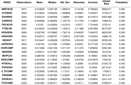
Descriptive statistics for the daily log returns for the selected indices are given in Table 1. All of the returns distributions are leptokurtic and the majority are negatively skewed. The Jarque-Bera test results indicate that none of the log returns series follows a Gaussian distribution15. The absolute value of the log-returns is significantly positively auto-correlated for a high number of lags. Examining the correlograms for the various indices, the decay in the value of the autocorrelation coefficients is initially rapid, before slowing and is suggestive of the hyperbolic decay which is typical for a long memory volatility process16.

[Insert Table 1 about here]

5. Empirical Analysis

VaR Analysis

14_{The estimations were carried out using the G@RCH (Laurent, 2009) for Ox programming language.}

15_{The unconditional distribution of the log-returns is not assumed to be the normal one. Under our model} framework, the log-returns are assumed to be conditionally, to the information set, normally distributed, i.e.







2



1 1 1 0

1~ 1 ,

| t t t

t I Nc c cy

y      . However, Bollerslev and Wooldridge's (1992) quasi-maximum likelihood

covariances and standard errors are estimated. If the assumption of conditional normality does not hold, the quasi-maximum likelihood parameter estimates of conditional variance will still be consistent, provided that the mean and variance functions are correctly specified.

(13)

The results for the one-step-ahead VaR forecasting across the 20 indices for both the FIGARCH and GARCH specifications are shown in Table 2. Overall, the fractionally integrated modelling of conditional volatility does not appear to improve the forecasting accuracy of VaR across the 20 stock indices for the one-step-ahead time horizon. Furthermore, the results appear to corroborate the findings from the literature that VaR models are not robust across different markets, so that the optimal model varies from one index to the next (Angelidis et al., 2004; McMillan and Kambouroudis, 2009).

According to the results of the Kupiec (1995) test, the observed violation rate is not statistically different to the expected violation rate (5%) for the one-step-ahead VaR forecasts produced by both the GARCH and FIGARCH models for the ATXINDX, GRAGENL, HNGKNGI, MXIPC35, POPSIGN, and S&PCOMP indices. This is also the case for the one-step-ahead VaR forecasts produced by the FIGARCH specification for the JAPDOWA and MADRIDI indices, and for the one-step-ahead VaR forecasts produced by the GARCH model for the DJINDUS index. In general, the models appear to underestimate the true VaR figure, as the observed proportion of VaR violations exceeds the expected value of 5% in almost all cases, sometimes by a large amount. This is in accordance with the findings of Kuester et al. (2006) who report that the majority of VaR models suffer from excessive VaR violations due to the models underestimating the true VaR figure.

According to the Christoffersen (1998) test, the VaR violations are independently distributed for the majority of the stock indices for both models, with just one exception, that of the ATXINDX for the FIGARCH



1,d,1



specification. However, although there is limited

evidence of clustering of the VaR violations, this is overridden by the results of the Kupiec test suggesting a widespread underestimation of the true VaR figure by both models.

(14)

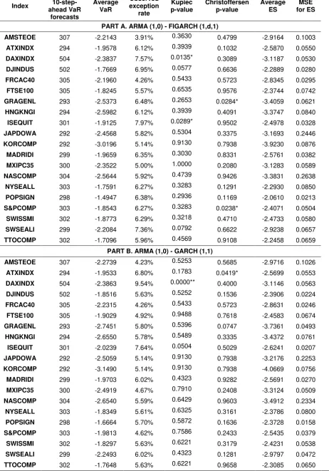
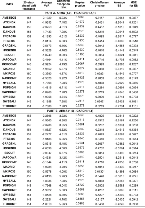
Table 4 shows the results for the forecasting of 20-step-ahead VaR across the 20 indices for both the FIGARCH and GARCH models. For this longer time horizon the performance of the FIGARCH model slightly improves from the 10-step-ahead forecasting period, as the Kupiec test results suggest that the observed exception rate is not statistically different to the expected failure rate for all the indices. Furthermore, the Christoffersen test results suggest that for two of these indices, namely the MXIPC35 and SWSEALI, the VaR violations are not independently distributed. A similar case holds for the performance of the GARCH model. It is now only marginally better than that of the FIGARCH model, with the Kupiec test indicating an adequate forecasting performance for all the 20 indices, but with one (MXIPC35) index showing evidence of clustering of VaR violations according to the Christoffersen test.

Another emerging pattern suggests that the longer the VaR forecasting time horizon, the less both models underestimate the true VaR. For the 1-day ahead time horizon, the observed failure rate was more than 5% in all 20 cases for the FIGARCH model and in 19 cases for the GARCH specification. At the 10-day-horizon the observed failure rate exceeded 5% in 18 cases (FIGARCH) and 15 cases (GARCH), whilst for the 20-day horizon the observed failure rate exceeded 5% in 13 and 11 cases for the FIGARCH and GARCH models, respectively.

Expected Shortfall Analysis

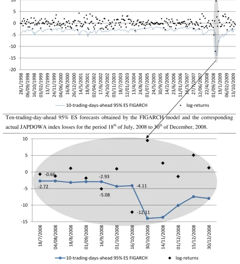
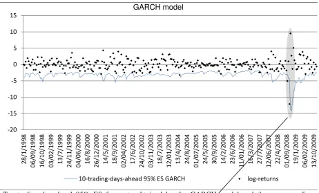
The ES measure reports to the risk manager the expected loss of his investment if an extreme event occurs; in other words, the capital requirement under stress test conditions. Figures 1 and 2 plot, indicatively, the non-overlapping 10-trading-days-ahead 95% ES forecasts for the JAPDOWA index. In order to provide a more explanatory review of the 95% ES forecasts, we focus on a specific period which is characterized by high volatility. The second part of Figures 1 and 2 provides a magnified illustration for the specific volatile period, which is indicated in the bubble scheme17.

17_{For example, for the trading day 18}th_{of July, 2008, for a portfolio of ¥10.000.000, the predicted amount of the}

(15)

[Insert Figure 1 about here] [Insert Figure 2 about here]

Turning to the estimates for the quadratic loss function that measures the distance between actual returns and expected returns in the event of a VaR violation (MSE for ES), the FIGARCH model produces lower values for the 1-day horizon for 13 of the indices. However, the GARCH model produces a lower MSE for ES values for 17 and 15 of the indices for the 10-day and 20-day forecasting horizons, respectively. These results corroborate the earlier results from the Kupiec and Christoffersen tests, that the performance of the two models is similar for the 1-day horizon, whilst the GARCH model slightly outperforms the long memory FIGARCH model for the 10-day and 20-day horizons. Therefore, accounting for long memory does not appear to improve the model’s ability to accurately forecast losses, and consequently the short memory GARCH specification is preferable since it is the more parsimonious model.

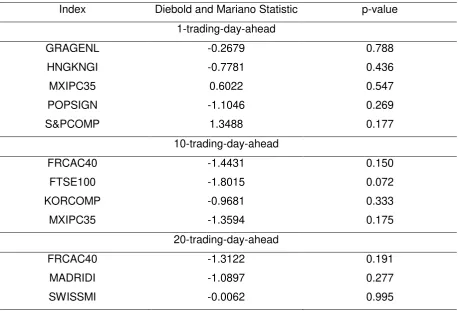
The Diebold and Mariano (1995) test is applied in order to investigate whether the difference between the MSE loss functions of GARCH and FIGARCH models is statistically significant. The null hypothesis of no difference in the forecasting accuracy of GARCH and FIGARCH models,



 tFIGARCH



0

GARCH t

E _ _ , is tested against the alternative

   





0

:

1   

FIGARCH t GARCH t

E

H _ _ . A negative value of the loss differential

 



  FIGARCH



t GARCH t FIGARCH GARCH

t   

 ,

indicates that the GARCH model provides a lower value of MSE for ES than the FIGARCH model18. The Diebold and Mariano statistic is computed as the t-statistic of regressing GARC HFIGARC H

t ,

 

 on a constant under the assumption

of Newey and West's (1987) heteroskedastic and autocorrelated consistent standard errors. Table 5 presents the Diebold and Mariano statistics and the relative p-values, indicatively, for indices that both GARCH and FIGARCH models forecast the 95% VaR accurately according to the Kupiec and Christoffersen tests. In all the cases, without any exception, the null hypothesis that the GARCH and FIGARCH models provide statistically equal MSE loss functions for Expected Shortfall forecasts is not rejected. Therefore, the long memory modelling of conditional volatility does not appear to improve the forecasting accuracy of ES, even for longer forecasting horizons.

18_{If the loss differential is a covariance-stationary short-memory process, then the Diebold and Mariano}

statistic,  



 

   _



  / _

~

1 , 1

, ~ T

t

FIGARCH GARCH t FIGARCH

GARCH

T , is asymptotically normally distributed, or

   

_{ }

1 , 0 ~

2 / 1 ,

,

N V GARCHFIGARCH

FIGARCH

GARCH 

   



 _

  

 

(16)

Rolling-sampled Parameter Estimates

A further aim of this study is to investigate the behaviour of the rolling-sampled estimated parameters over time. The topic of constancy of parameters across time is a long-standing historical debate as old as the role of econometrics in economics. Hendry (1996) notes : "The parameter is constant over the time period T if it has the same value for all

T

t . ... As the historical debate19 showed, constancy has long been regarded as a fundamental requirement for empirical modelling. ... Keynes claimed a number of ‘pre

-conditions’ for the validity of inferences from data, including both ‘time homogeneity’ (or

parameter constancy) and a complete prior theoretical analysis, so he held to an extreme

form of the ‘axiom of correct specification’ (see Leamer, 1978): statistical work in economics

was deemed impossible without prior theoretical knowledge. ... However, as argued in

Hendry (1995), if partial explanations are devoid of use (i.e., we cannot discover empirically

anything that is not already known theoretically), Keynes must have believed no science ever

progressed."

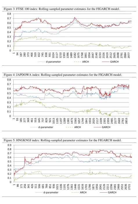
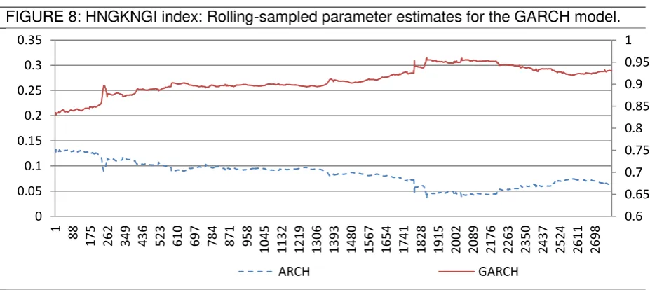
Due to the fact that news information arrives daily in an unpredictable fashion, the estimated parameters should be revised on a daily basis (see Engle et al., 1990; Degiannakis et al., 2008). Figures 3 to 8 illustrate the time plot of the rolling-sampled estimated parameters from the FIGARCH and GARCH models. In our case, there is evidence of a considerable time-varying characteristic of the estimated parameters of both models for FTSE-100, JAPDOWA and HNGKNGI indices20. Test statistics, i.e. Andrews (1993) and Bai and Perron (1998), would reject the hypothesis of constancy of parameters of both models across various subsamples.

[Insert Figures 3-8 about here]

However, the research question arises: Why do long memory FIGARCH models have more time-varying parameters than the short memory GARCH models? Meitz and Saikkonen (2008) give conditions under which the AR(1)-GARCH(1,1) model is stable in the sense that its Markov chain representation is geometrically ergodic. Although, there is no previous

19_{The historical debate refers to Robbins (1932), Keynes (1939) Frisch (1938), and Hendry and Morgan (1995),}

among others.

20_{The time-varying characteristic of the estimated parameters holds for all 20 indices. Figures for other indices}

(17)

evidence on the stability of FIGARCH parameters, we show that these parameters change less smoothly over time compared to the GARCH models.

Hence, we observe that the estimated parameters of the FIGARCH model exhibit a relatively more time-varying characteristic than those of the GARCH model. Not all of the instability can be due to the news information arrival process of the market since both models are fitted to data from the same sample period; a portion must be due to the FIGARCH modelling process itself.

6. Conclusion and Suggestions for Further Research

This research has examined whether or not accounting for fractional integration in the volatility process improves VaR and ES forecasting performances, particularly as the forecasting time horizon lengthens. To this end, the paper proposes the application of the Monte Carlo simulation technique of Christoffersen (2003) to estimating multiple-step-ahead VaR forecasts using the FIGARCH model. The models were tested across 20 leading stock indices worldwide over the period from 1989 to 2009, at the 95% confidence level, for the 1-step-ahead, 10-step-ahead and 20-step-ahead VaR forecasts.

The modelling results suggest that despite evidence of persistence in the volatility process, accounting for long memory in the model did not improve the VaR and ES forecasting accuracy relative to the short memory specification. Kuester et al. (2006) find that the majority of VaR models suffer from excessive VaR violations, implying an underestimation of market risk. Our results suggest that for both modelling specifications underestimation of the true VaR becomes less prevalent as the forecasting time horizon increases.

In addition, the time-varying property of the rolling-sampled FIGARCH parameters estimates appear not to be due solely to the news information arrival process on the market, but a portion must be due to the FIGARCH modelling process itself. The manuscript concludes that the models should be constructed carefully, either by risk managers or by market regulators. The ES estimates the capital requirements when a violation of normal market conditions occurs. The forecast of such measures must not be based on fractionally integrated models before their forecasting ability has been investigated. The incorporation of the long memory property in volatility modelling is not a panacea.

(18)

forecast period. As a result, particularly for the 20-day time horizon, the results of the Kupiec and Christoffersen tests are highly sensitive to the number of VaR violations such that a very small number of additional (or fewer) violations can be pivotal in determining whether or not the forecasting performance of the model is deemed to be adequate. Furthermore, the Kupiec model has been shown to lack power when the number of observations is small (Crouhy et al., 2001).

The models presented in this paper were estimated under the assumption of normally21 distributed standardised residuals, since this distribution has fewer parameters and allowed the focus of the research to be on the relative VaR forecasting performances of the long memory and short memory specifications. Overall, in the literature, the long memory volatility models provide a superior one-day-ahead forecasting performance, in cases that the long memory is combined with skewed distribution. Degiannakis (2004) provides evidence that a fractionally integrated asymmetric ARCH model with skewed Student-t conditionally distributed innovations forecasts 1-day-ahead VaR adequately. The adaptive FIGARCH specification, of Baillie and Morana (2009), which accounts for both long memory and structural changes within the conditional variance process, outperforms the FIGARCH model in the presence of structural breaks, whilst the parameters of the model are less biassed and more efficient compared to those of a FIGARCH specification. Future research may incorporate multi-day-ahead VaR and ES forecasts allowing for asymmetry in the returns' distribution, i.e. the skewed Student-t, which has been suggested to improve VaR forecasting accuracy (Giot and Laurent 2003, and 2004; Tang and Shieh, 2006; McMillan and Kamboroudis, 2009).

Further research might benefit from the use of intra-daily data since the longer time series would increase the number of observations and will strengthen the results, particularly for longer forecasting time horizons. The emerging observation that the underestimation of the true VaR becomes less prevalent as the forecasting time horizon increases also warrants further investigation.

Acknowledgement

We thank the participants of the 17th Annual Conference of the Multinational Finance Society, in Barcelona, for their comments, and especially Professor Johan Kniff from the

(19)

Hanken School of Economics for his valuable suggestions. Dr. Christos Floros and Dr.

Stavros Degiannakis acknowledge the support from the European Community’s Seventh Framework Programme (FP7-PEOPLE-IEF) funded under grant agreement no. PIEF-GA-2009-237022.

References

Andrews, D.K (1993). Tests for parameter instability and structural change with unknown change point. Econometrica, 61,4, 821-856.

Angelidis, T., Benos, A. and Degiannakis, S. (2004). The use of GARCH models in VaR estimation. Statistical Methodology, 1, 105-128.

Angelidis, T. and Degiannakis, S. (2007). Backtesting VaR models: a two-stage procedure.

Journal of Risk Model Validation, 1 (2), 1-22.

Artzner, P., Delbaen, F., Eber, J. and Heath, D., (1997). Thinking Coherently. Risk, 10, 68-71.

Artzner, P., Delbaen, F., Eber, J. and Heath, D., (1999). Coherent Measures of Risk.

Mathematical Finance, 9 (3), 203-228.

Bai, J. and Perron, P. (1998). Estimating and testing linear models with multiple structural changes. Econometrica, 66,1, 47-78.

Baillie, R., Bollerslev, T. and Mikkelsen, H. (1996). Fractionally integrated generalised autoregressive conditional heteroscedasticity. Journal of Econometrics, 74, 3-30.

Baillie R. and Morana, C. (2009). Modelling long memory and structural breaks in conditional Variances: An adaptive FIGARCH approach. Journal of Economic Dynamics and Control, 33, 1577-1592.

Basel Committee on Banking Supervision (1996). Amendment to the Capital Accord to incorporate Market Risks. Basel.

Basel Committee on Banking Supervision (2006). International Convergence of Capital Measurement and Capital Standards – A Revised Framework. Basel.

Basel Committee on Banking Supervision (2009). Revisions to the Basel II Market Risk Framework. Basel.

Bollerslev, T. (1986). Generalised autoregressive conditional heteroscedasticity. Journal of Econometrics, 31, 307-327.

(20)

Bollerslev, T. and Wooldridge, J.M. (1992). Quasi-maximum Likelihood Estimation and Inference in Dynamic Models with Time-Varying Covariances. Econometric Reviews, 11, 143-172.

Brooks, C. and Persand, G. (2003). Volatility Forecasting for Risk Management. Journal of Forecasting, 22, 1-22.

Caporin, M. (2008). Evaluating Value-at-Risk measures in presence of long memory conditional volatility, Journal of Risk, 10(3), 79-110.

Chen, Y. and Lu, J. (2010). Value at Risk Estimation, Chapter in Handbook of Computational Finance (Eds: Duan, J-C, Gentle, J.E. and Hardle, W.), Springer.

Christoffersen, P. (1998) Evaluating interval forecasts. International Economic Review, 39,

841-862.

Christoffersen, P. (2003). Elements of Financial Risk Management. CA: Elsevier Science. Crouhy, M., Galai, D. and Mark, R. (2001). Risk Management. McGraw-Hill, New York. Danielsson, J. and Morimoto, Y. (2000). Forecasting extreme financial risk: A critical

analysis of practical methods for the Japanese market. Monetary and Economic Studies, 18(2), 25-48.

Degiannakis, S. (2004). Volatility forecasting: evidence from a fractional integrated asymmetric power ARCH skewed-t model. Applied Financial Economics, 14, 1333-1342. Degiannakis, S., Livada, A. and Panas, E. (2008). Rolling-sampled parameters of ARCH and

Levy-stable models. Applied Economics, 40, 3051-3067.

Diebold, F.X. and Mariano, R. (1995). Comparing Predictive Accuracy. Journal of Business and Economic Statistics, 13(3), 253-263.

Dionne, G., Duchesne, P. and Pacurar, M. (2009). Intraday Value at Risk (IVaR) using tick-by-tick data with application to the Toronto Stock Exchange, Journal of Empirical Finance, 16, 777-792.

Dowd, K. (2002). Measuring Market Risk. John Wiley & Sons, New York.

Ellis, C. And Wilson, P. (2004). Another look at the forecast performance of ARFIMA models. International Review of Financial Analysis, 13, 63-81.

Engle, R.F. (1982). Autoregressive conditional heteroskedasticity with estimates of the variance of UK inflation. Econometrica, 50, 987-1008.

Engle, R.F. (2004). Risk and Volatility: Econometric Models and Financial Practice. The American Economic Review, 94 (3), 405-420.

(21)

Frisch, R. (1938). Statistical versus theoretical relations in economic macrodynamics. Mimeograph dated 17 July 1938, League of Nations Memorandum.

Giot, P. and Laurent, S. (2003). Value-at-Risk for Long and Short Trading Positions. Journal of Applied Econometrics, 18 (6), 641-664.

Giot, P. and Laurent, S. (2004). Modelling daily Value-at-Risk using realised volatility and ARCH type models. Journal of Empirical Finance, 11, 379-398.

Granger, C. and Hyung, N. (2004). Occasional structural breaks and long memory with an application to the S&P500 absolute returns, Journal of Empirical Finance, 11, 399-421. Halbleib, R. and Pohlmeier, W. (2012). Improving the value at risk forecasts: Theory and

evidence from the financial crisis, Journal of Economic Dynamics & Control, 36, 1212-1228.

Hansen, P.R. and Lunde, A. (2005). A Forecast Comparison of Volatility Models: Does Anything Beat a GARCH(1,1)? Journal of Applied Econometrics, 20(7), 873-889.

Härdle, W. and Mungo, J., (2008). Value-at-Risk and Expected Shortfall when there is long range dependence. SFB 649, Discussion Paper 2008-006, Humboldt-universität zu Berlin, Germany.

Harris, R. and Sollis, R. (2003). Applied Time Series Modelling and Forecasting. John Wiley & Sons, New York.

Hendry, D.F. (1995). Econometrics and business cycle empirics. Economic Journal, 105, 1622–1636.

Hendry, D.F. (1996). On the Constancy of Time-Series Econometric Equations. Economic and Social Review, 27, 401-422.

Hendry, D.F., and Morgan, M.S. (1995). The Foundations of Econometric Analysis. Cambridge University Press, Cambridge.

Hoppe, R. (1999). Finance is not Physics. Risk Professional, 1(7).

Keynes, J.M. (1939). Professor Tinbergen’s method. Economic Journal, 44, 558–568.

Kuester, K. Mittnik, S. and Paolella, M.S. (2006). Value-at-Risk prediction: a comparison of alternative strategies. Journal of Financial Econometrics, 4(1), 53-89.

Kupiec, P. (1995). Techniques for verifying the accuracy of risk measurement models.

Journal of Derivatives, 2, 73-84.

Laurent, S. (2009). G@RCH 6. Estimating and Forecasting GARCH Models. Timberlake Consultants Press, London.

(22)

Lo, A. and MacKinlay, A.C. (1990). An Econometric Analysis of Non-synchronous Trading.

Journal of Econometrics, 45, 181-212.

McMillan, D. and Kambouroudis, D. (2009). Are Riskmetrics forecasts good enough? Evidence from 31 stock markets. International Review of Financial Analysis, 18, 117-124. McMillan, D. and Ruiz, I. (2009). Volatility persistence, long memory and time-varying

unconditional mean: Evidence from 10 equity indices. The Quarterly Review of Economics and Finance, 49, 578-595.

Meitz, M. and Saikkonen, P. (2008). Stability of non-linear AR-GARCH models. Journal of Time Series Analysis, 29 (3), 453-475.

Nagayasu, J. (2008). Japanese Stock Movements from 1991-2005: evidence from high- and low-frequency data. Applied Financial Economics, 18 (4), 295-307.

Newey, W. and West, K.D. (1987). A Simple Positive Semi-Definite, Heteroskedasticity and Autocorrelation Consistent Covariance Matrix. Econometrica, 55, 703-708.

Robbins, L. (1932). An Essay on the Nature and Significance of Economic Science. Macmillan, London.

Rossignolo, A. F., Fethi, M. D. and Shaban, M. (2011). Value-at-Risk models and Basel capital charges: Evidence from Emerging and Frontier stock markets. Journal of Financial Stability. in press.

Semenov, A. (2009). Risk factor beta conditional Value-at-Risk. Journal of Forecasting. 28(6), 549-558.

Shao,X.-D., Lian Y.-J. and Yin, L.-Q. (2009). Forecasting Value-at-Risk using high frequency data: The realized range model. Global Finance Journal. 20(2), 128-136.

Sriananthakumar, S. and Silvapulle, S. (2003). Estimating value at risks for short and long trading positions. Working paper, Department of Economics and Business Statistics, Monash University, Australia.

Taleb, N. (1997). Against VaR. Derivatives Strategy, April.

Tang, T. and Shieh, S. (2006). Long memory in stock index futures markets: A value-at-risk approach. Physica A, 366, 437-448.

Xekalaki, E. and Degiannakis, S. (2010). ARCH Models for Financial Applications. John Wiley & Sons, New York.

(23)

Appendix

Based on Xekalaki and Degiannakis (2010) and Christoffersen (2003), a Monte Carlo simulation algorithm for computing (95%)

|t t

VaR__ and (95%) |t t

ES__ based on fractionally integrated conditional volatility model is presented. Consider the AR(1)-FIGARCH(1,1):





t t

t c c c y

y  ₀ 1 ₁  ₁ _₁

t t t  z

 

 

0,1 ~N z_t









1 21,

1 2 1 1 2 2 1 1 1 0 2          





t

j t t j j t

t a a b   L  a b



(A1)

The  -day-ahead 95% VaR and Expected Shortfall estimates are obtained as:

One-day-ahead

 Step 1.1. Compute the one-day-ahead conditional variance as

 



   



 



 



 











 



1  2| 1 2 | 1 2 | 1 2 | 1 1 0 | 1 1

1 tt

t j j t t t j t t j t t t t t t t t t

t L a b

j d d j d b a

a    

 _                



      (A2)

 Step 1.2. Generate 5.000 random numbers

 

5000 1 1 , _i_ i z



from the standard normal distribution

 Step 1.3. Create the hypothetical returns of time t1 , as

 



 



  1 , | 1 1 1 0 1

, 1 t t t i

t t t t

i c c c y z

y _     _  , for i 1,,5.000 Two-day-ahead

 Step 2.1. Create the forecast variance for time t2, 2 2 ,t i



 Step 2.2. Generate 5.000 random numbers,

 

zi,2 5_i_.000₁



, from the standard normal distribution

 Step 2.2. Calculate the hypothetical returns of time t2 ,

 



 



  2 , 2 , 1 , 1 1 0 2

, 1 it it i

t t t t

i c c c y z

y   



 

     , for i 1,,5.000

Three-day-ahead

 Step 3.1. Create the forecast variance for time t3, 2 3 ,t i



 Step 3.2. Generate 5.000 random numbers,

 

zi,3 5_i_.000₁



(24)

 Step 3.3. Calculate the hypothetical returns of time t3 ,

 



 



 

3 , 3 , 2 , 1 1 0 3

, 1 it it i

t t t t

i c c c y z

y _     _  _  , for i 1,,5.000

…

 -day-ahead

 Step  .1. Generate 5.000 random numbers,

 

5.000 1 , _i_ i z _



, from the standard normal distribution

 Step  .2. Calculate the hypothetical returns of time

t





,

 



 



 

  

 0 1 1 , 1 , ,

, 1 it it i

t t t t

i c c c y z

y _     _ _   _ 

Step  .3. Calculate the  -day-ahead 95% VaR as



 

5000



1 , % 5 %) 95 (

| f  _

 t  it i

t y

VaR    and

the  -day-ahead 95% ES as





 





    



  k

i

k i t t t

t k VaR

ES

~

1

) 1 ~ 05 . 0 05 . 0 1 (

| 1

%) 95 (

|

1 ~

(25)

[image:25.595.47.554.126.454.2]

Figures and Tables

Table 1: Descriptive Statistics.

INDEX Observations Mean Median Std. Dev. Skewness Kurtosis

Jarque-Bera Probability

1

AMSTEOE 5072 0.016836 0.067192 1.395972 -0.16156 9.766062 9696.817 0.000 ATXINDX 4945 0.019052 0.054244 1.408684 -0.28461 10.83047 12700.47 0.000 DAXINDX 5044 0.025316 0.083406 1.48699 -0.12667 8.012514 5293.989 0.000 DJINDUS 5029 0.026568 0.049052 1.125719 -0.11793 11.44804 14966.53 0.000 FRCAC40 5050 0.0135 0.033854 1.412313 -0.0377 7.751845 4752.41 0.000 FTSE100 5051 0.016534 0.040528 1.150512 -0.11488 9.561969 9073.327 0.000 GRAGENL 4936 0.032748 0.018962 1.736119 0.044387 7.844572 4828.592 0.000 HNGKNGI 4944 0.042274 0.062797 1.725812 0.007238 12.05344 16884.78 0.000 ISEQUIT 5017 0.010447 0.049028 1.257524 -0.65183 13.22265 22200.69 0.000 JAPDOWA 4924 -0.02745 -0.01268 1.578394 -0.02021 8.277182 5713.949 0.000 KORCOMP 4924 0.011606 0.041168 1.911157 -0.11475 7.005832 3303.052 0.000 MADRIDI 4992 0.02815 0.077387 1.283485 -0.20082 8.496868 6318.39 0.000 MXIPC35 5003 0.088184 0.103812 1.640208 0.029248 8.16869 5569.752 0.000 NASCOMP 5042 0.031029 0.114602 1.57385 -0.04783 8.913875 7349.36 0.000 NYSEALL 5035 0.025034 0.058148 1.122936 -0.3696 15.23759 31532.73 0.000 POPSIGN 4984 0.021379 0.018262 0.966043 -0.42194 15.9026 34719.61 0.000 S_PCOMP 5039 0.022856 0.048103 1.17312 -0.19843 12.1539 17626.3 0.000 SWISSMI 5023 0.025303 0.067464 1.218007 -0.14656 9.126867 7874.477 0.000 SWSEALI 4999 0.030183 0.066004 1.393286 0.148244 7.555802 4341.474 0.000 TTOCOMP 5029 0.021684 0.061911 1.055662 -0.76711 14.25989 27059.97 0.000

1

(26)

[image:26.595.75.523.83.744.2]

Table 2: 1-step-ahead VaR and ES modelling results.

Index

Number of 1-step-ahead VaR forecasts

Average VaR

Observed exception

rate

Kupiec p-value

Christoffersen p-value

Average ES

MSE for ES

PART A. ARMA (1,0) - FIGARCH (1,d,1)

AMSTEOE 3072 -2.279 5.99% 0.0145* 0.5369 -2.873 0.041 ATXINDX 2945 -2.009 5.57% 0.1639 0.0278* -2.534 0.042 DAXINDX 3044 -2.426 6.47% 0.0004** 0.3937 -3.059 0.040 DJINDUS 3029 -1.832 5.81% 0.0458* 0.5662 -2.310 0.036 FRCAC40 3050 -2.252 6.36% 0.0009** 0.4328 -2.838 0.038 FTSE100 3051 -1.889 5.97% 0.0174* 0.3296 -2.378 0.027

GRAGENL 2936 -2.553 5.48% 0.2361 0.1624 -3.210 0.052

HNGKNGI 2944 -2.638 5.40% 0.3243 0.8833 -3.325 0.068

ISEQUIT 3017 -2.015 6.20% 0.0035** 0.6102 -2.260 0.060

JAPDOWA 2924 -2.483 5.75% 0.0705 0.9069 -3.117 0.050

KORCOMP 2924 -3.112 6.12% 0.0071** 0.9902 -3.914 0.101

MADRIDI 2992 -2.019 5.51% 0.2035 0.6936 -2.550 0.035

MXIPC35 3003 -2.415 5.46% 0.2529 0.4732 -3.059 0.047

NASCOMP 3042 -2.665 6.48% 0.0003** 0.2375 -3.361 0.044 NYSEALL 3035 -1.815 5.83% 0.0402* 0.1448 -2.289 0.029

POPSIGN 2984 -1.528 5.76% 0.0613 0.7195 -1.929 0.038

S&PCOMP 3039 -1.930 5.76% 0.0608 0.7135 -2.434 0.032 SWISSMI 3023 -1.919 6.42% 0.0006** 0.6541 -2.423 0.032 SWSEALI 2999 -2.255 5.80% 0.0492* 0.7090 -2.852 0.039 TTOCOMP 3029 -1.754 6.50% 0.0003** 0.2309 -2.214 0.043

PART B. ARMA (1,0) - GARCH (1,1)

AMSTEOE 3072 -2.272 6.28% 0.0017** 0.2553 -2.863 0.0441 ATXINDX 2945 -1.967 5.74% 0.0721 0.1665 -2.481 0.0457 DAXINDX 3044 -2.391 6.73% 0.0000** 0.0715 -3.015 0.0422 DJINDUS 3029 -1.844 5.55% 0.1748 0.8158 -2.326 0.0343 FRCAC40 3050 -2.234 6.43% 0.0005** 0.8558 -2.815 0.0379 FTSE100 3051 -1.895 6.33% 0.0012** 0.2666 -2.386 0.0299

GRAGENL 2936 -2.596 4.97% 0.9459 0.3093 -3.264 0.0513

HNGKNGI 2944 -2.623 5.71% 0.0851 0.4251 -3.306 0.0649

(27)

[image:27.595.60.523.84.746.2]

Index

Number of 10-step-ahead VaR

forecasts

Average VaR

rate

Average ES

MSE for ES

AMSTEOE 307 -2.2143 3.91% 0.3630 0.4799 -2.9164 0.1003 ATXINDX 294 -1.9578 6.12% 0.3939 0.1032 -2.5870 0.0550 DAXINDX 504 -2.3837 7.57% 0.0135* 0.3089 -3.1187 0.0530 DJINDUS 502 -1.7669 6.95% 0.0577 0.6636 -2.2889 0.0280 FRCAC40 305 -2.1960 4.26% 0.5433 0.5723 -2.8345 0.0295 FTSE100 305 -1.8245 5.57% 0.6535 0.9576 -2.3744 0.0742 GRAGENL 293 -2.5373 6.48% 0.2653 0.0284* -3.4059 0.0621 HNGKNGI 294 -2.5982 6.12% 0.3939 0.4091 -3.3747 0.0840 ISEQUIT 301 -1.9125 7.97% 0.0289* 0.9502 -2.4978 0.0328 JAPDOWA 292 -2.4568 5.82% 0.5304 0.3375 -3.1693 0.2446 KORCOMP 292 -3.0196 5.14% 0.9130 0.7938 -3.9230 0.0876 MADRIDI 299 -1.9659 6.35% 0.3030 0.8331 -2.5761 0.0382 MXIPC35 300 -2.3522 5.00% 1.0000 0.2080 -3.1283 0.0589 NASCOMP 304 -2.5644 5.92% 0.4739 0.9426 -3.3831 0.2638 NYSEALL 303 -1.7591 6.27% 0.3283 0.1291 -2.2930 0.0850 POPSIGN 298 -1.4947 6.38% 0.2936 0.1169 -2.0610 0.0213 S&PCOMP 303 -1.8543 6.27% 0.3283 0.0238* -2.4071 0.0504 SWISSMI 302 -1.8773 6.29% 0.3218 0.4710 -2.4733 0.0580 SWSEALI 299 -2.2084 7.36% 0.0792 0.6622 -2.9238 0.0657 TTOCOMP 302 -1.7096 5.96% 0.4569 0.9108 -2.2458 0.0659

PART B. ARMA (1,0) - GARCH (1,1)

(28)

[image:28.595.58.527.80.751.2]

Index

Number of 20-step-ahead VaR

forecasts

Average VaR

rate

Average ES

MSE for ES

AMSTEOE 153 -2.1929 5.23% 0.8969 0.3457 -2.9664 0.0837 ATXINDX 147 -1.9353 7.48% 0.1972 0.8431 -2.6041 0.1201 DAXINDX 152 -2.3759 4.61% 0.8232 0.4457 -3.1815 0.0349 DJINDUS 151 -1.7433 7.28% 0.2273 0.8219 -2.2948 0.1522 FRCAC40 152 -2.1893 4.61% 0.8232 0.4093 -2.8817 0.0727 FTSE100 152 -1.8114 6.58% 0.3930 0.1414 -2.4085 0.0518 GRAGENL 146 -2.5173 6.16% 0.5342 0.3042 -3.4558 0.0398 HNGKNGI 147 -2.5828 4.76% 0.8930 0.4010 -3.4149 0.0349 ISEQUIT 150 -1.8749 8.00% 0.1195 0.3054 -2.4824 0.0341 JAPDOWA 146 -2.4164 4.11% 0.6111 0.4716 -3.1703 0.0082 KORCOMP 146 -2.9924 4.79% 0.9067 0.3993 -3.9593 0.1267 MADRIDI 149 -1.9552 5.37% 0.8377 0.3388 -2.6116 0.0367 MXIPC35 150 -2.3390 4.67% 0.8513 0.0282* -3.1549 0.0707 NASCOMP 152 -2.5020 5.92% 0.6126 0.2853 -3.3686 0.3173 NYSEALL 151 -1.7308 7.28% 0.2273 0.1868 -2.2929 0.0356 POPSIGN 149 -1.4615 6.71% 0.3616 0.2284 -2.0694 0.0094 S&PCOMP 151 -1.8266 7.28% 0.2273 0.8219 -2.4045 0.0400 SWISSMI 151 -1.9058 4.64% 0.8373 0.3090 -2.5744 0.0793 SWSEALI 149 -2.1658 7.38% 0.2117 0.0342* -2.9428 0.1061

TTOCOMP 151 -1.7006 7.28% 0.2273 0.8219 -2.2734 0.1151

PART B. ARMA (1,0) - GARCH (1,1)

AMSTEOE 153 -2.2896 3.92% 0.5248 0.4825 -3.0813 0.0222 ATXINDX 147 -1.9360 6.80% 0.3413 0.1512 -2.6161 0.1250 DAXINDX 152 -2.3736 3.95% 0.5381 0.5207 -3.1831 0.0233 DJINDUS 151 -1.8627 6.62% 0.3832 0.2318 -2.4515 0.1364 FRCAC40 152 -2.2477 4.61% 0.8232 0.4093 -2.9269 0.0627 FTSE100 152 -1.9136 5.26% 0.8840 0.3440 -2.5249 0.0644 GRAGENL 146 -2.8315 5.48% 0.7931 0.3667 -4.0362 0.0643 HNGKNGI 147 -2.6596 4.08% 0.5975 0.4732 -3.5204 0.0514 ISEQUIT 150 -2.0047 6.67% 0.3708 0.6854 -2.6492 0.0244 JAPDOWA 146 -2.4931 3.42% 0.3540 0.5501 -3.2518 0.0043 KORCOMP 146 -3.1844 4.11% 0.6111 0.4716 -4.2056 0.0768 MADRIDI 149 -1.9788 4.70% 0.8653 0.4044 -2.6439 0.0217 MXIPC35 150 -2.5278 4.00% 0.5610 0.0130* -3.4393 0.0684 NASCOMP 152 -2.6196 5.26% 0.8840 0.3440 -3.5615 0.2221 NYSEALL 151 -1.8336 7.28% 0.2273 0.1868 -2.4266 0.0321 POPSIGN 149 -1.7368 6.04% 0.5722 0.2802 -2.6582 0.0289 S&PCOMP 151 -1.9922 5.30% 0.8669 0.4207 -2.6065 0.0111 SWISSMI 151 -1.8528 5.30% 0.8669 0.4207 -2.5202 0.0793 SWSEALI 149 -2.2321 4.70% 0.8653 0.3137 -3.0435 0.0942