Munich Personal RePEc Archive
(Ir)rational Voters?
Spenkuch, Jörg
Northwestern University
November 2014
Online at
https://mpra.ub.uni-muenchen.de/60100/
(Ir)rational Voters?
J•org L. Spenkuch
Northwestern University
November 2014
Abstract
Social scientists have long speculated about the extent of agents' rationality, espe-cially in the context of voting. However, existing attempts at classifying voters as (ir)rational have been hampered by the fact that preference orderings and, thus, optimal strategies are generally unobserved. Exploiting the incentive structure of Germany's electoral system, this paper develops a novel set of empirical tests in or-der to pit the canonical rational choice model against behavioral theories according to which voters simply choose their most preferred candidate. The results indicate that neither approach can rationalize the most-salient features of the data. The ndings are consistent, however, with a simple hybrid model in which boundedly rational agents su er a small psychic cost from acting strategically.
1. Introduction
Rational choice theory is, without question, the dominant paradigm in economics and much of political science. Even issues once thought to be far beyond the realm of traditional economics have long been analyzed through the lens of rational choice (see, e.g., Becker 1993). At the same time, a large behavioral literature suggests that agents face cognitive constraints, and that deviations from strict, unbounded rationality may matter for many real-world outcomes (Simon 1955, 1972; see also the surveys by Conlisk 1996; Camerer 2006; and DellaVigna 2009). If economics is to be a positive science of actual human behavior|as opposed to a normative one of how people should behave|then understanding how prevalent these deviations are is a matter of rst-order importance.
An area of economics within which scholars have long been interested in this question is social choice (e.g., Black 1948; Downs 1957; Duverger 1954; Farquharson 1969; Sen 1970). On the one hand, practically every reasonable electoral system fails to be strategy-proof, and voters are known to have a systematic incentive to misrepresent their true preferences in order to a ect the outcome of an election (Arrow 1951; Gibbard 1973; Satterthwaite 1975). On the other hand, pivot probabilities in large elections are often vanishingly small. If voters su er even a small cost from abandoning their favorite candidate or from determining their optimal strategy, then one may not expect any of them to act strategically (Downs 1957; Green and Shapiro 1994; Sen 1970).
Given the theoretical merits of both arguments, it may not be surprising that there exists no consensus on how voters actually behave. Some model voters as strategic, unboundedly rational individuals seeking to a ect electoral outcomes (e.g., Austen-Smith and Banks 1988; Besley and Coate 1997; Bouton 2013; Feddersen and Pesendorfer 1996). Others, however, cast voters as behavioral agents who na•vely choose their most preferred candidate, irrespective of her chances of winning (e.g., Callander 2005; Osborne and Slivinski 1996; Palfrey 1984). As practically all formal theories in which agents face more than two alternatives require an assumption about the rationality of individuals, and given that the conclusions from nearly identical models may depend critically on whether voters are taken to be strategic or sincere (compare, for instance, Besley and Coate 1997 with Osborne and Slivinski 1996), it is crucial to close this gap in knowledge. More generally, studying voter behavior in large elections with (arguably) weak electoral incentives helps to understand to what extent agents act \as if" they are unboundedly rational.
deviate from the underlying preference orderings. In fact, in an important paper, Degan and Merlo (2009) prove thatany cross section of votes can be explained by some utility function, without resorting to strategic behavior.
To illustrate the problem, consider the 2000 presidential election in Florida, in which George W. Bush beat out Al Gore by a margin of 537 votes, and as a result, won the U.S. presidency. Although Florida was widely expected to be a swing state, more than 138,000 voters chose third-party candidates. Viewed through the lens of the canonical rational choice model, these 138,000 voters could not have behaved strategically, as doing so would have required them to abandon their favorite candidate and vote for either Bush or Gore. Unfortunately, all one can infer from data like these is that at least 138,000 out of almost 6 million voters did not behave in accordance with standard theory.1 In order to derive
more meaningful results, one would ideally like to know how many voters actually prefered a third-party candidate, whom they should have abandoned in favor of Bush or Gore. With this information in hand, it would be straightforward to determine whether the observed number of \mistakes" is economically large or small.
Given the prominence of the pivotal voter model, i.e. the assumption of cognitively uncon-strained actors attempting to a ect the outcome of an election, this paper's primary goal is to quantify deviations from this baseline. As a matter of terminology, agents are said to be not instrumentally rational if they fail to abandon a candidate who has no chance of winning.
In order to circumvent the fundamental identi cation problem, the present paper exploits the incentive structure of parliamentary elections in Germany. Under the German system, individuals have two votes. Both are submitted simultaneously and are used to elect rep-resentatives to the same chamber of parliament. Critically, they are associated with very di erent incentives. Thelist vote is cast for a party and counted at the national level. Up to a rst-order approximation, list votes determine the distribution of seats in the Bundestag. Since mandates are awarded on a proportional basis (conditional on clearing a 5%-threshold), it is in most agents' best interest to reveal their (induced) preferences over which party they wish to gain the marginal seat by voting for said party.2
By contrast, the candidate vote is counted in a rst-past-the-post system at the district level. Whichever candidate wins the plurality of votes in a given district is automatically
1
Kawai and Watanabe (2013) call this \misaligned voting." Clearly, the set of agents who cast misaligned votes is only a (potentially small) subset of strategic voters, i.e. those who would abandon their preferred candidate if need be.
2
elected. Votes cast for any other contestant are \lost." Although the candidate vote is pri-marily used to determine the identity of local representatives, by securing a disproportionate share of districts parties may actually increase their seat totals (see Section 2 for details). The important point is that when it comes to choosing among di erent candidates, voters have a clear incentive to behave tactically. As in all elections under plurality rule, agents who act in accordance with standard rational choice theory should never vote for a party's nominee if she is known to be \out of the race." Only by choosing one of the candidates who remain in contention for victory can voters hope to a ect the outcome of the race.
Under the assumption that voters are not exactly indi erent about who carries their home district, it is possible to shed light on whether individual choices are consistent with leading theories of how voters behave. To see why the German context is helpful, consider an agent who cast his party vote for the small, libertarian FDP. Although the FDP elds candidates in practically all district-level races, they are almost never in contention for victory. Thus, as long as this voter knows that the FDP candidate in his district is \out of the race," he should not vote for her. Doing so would be inconsistent with instrumental rationality. Instead, conditional on supporting the FDP, he should split his ticket and vote for the candidate of another party|one who actually is in contention for victory.
While it is tempting to think of the list vote as a proxy for agents' preferences over parties and the associated candidates|especially if one believes that voters do not have strong incentives to behave strategically under proportional representation|it is important to emphasize at the outset that such an assumption is not required for testing rational choice theory. Voting for a candidate who is known to be \out of the race" is inconsistent with instrumental rationality, irrespective of why a given individual chose to support the associated party.
Hence, instead of asking the di cult question of what fraction of voters sticks with their preferred candidate despite her having no chance of winning, the German electoral system allows us to tackle a much simpler one: Conditional on having a strategic incentive to split their ballot, how many voters fail to do so? That is, how many of a party's supporters simply vote for the associated candidate despite her being \out of the race?"3
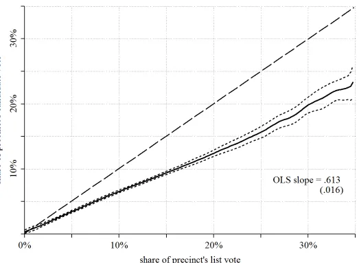
As Figure 1 demonstrates, the answer turns out to be \most." Restricting attention to candidates who trailed the runner-up by more than 10 percentage points, the gure displays a semiparametric estimate of the relationship between precinct-level vote shares of a candi-date's party and the candidate herself. If individuals behaved as prescribed by the standard
3
pivotal voter model and were not \irrationally" optimistic about these candidates' chances of being in contention for victory, then none of them should have gotten any votes, irrespective of how popular the party happened to be in a particular precinct. The data resoundingly reject this prediction. In fact, the slope estimate indicates that more than 60% of party supporters stick with candidates who are \out of the race."
This and all other ndings are based on previously unavailable, o cial precinct-level data from the 2005 and 2009 federal elections. In Germany, precincts are the smallest administra-tive units at which votes are counted, and each precinct is fully contained within one electoral district. Since races take place at the district level, these data allow for the use of within-candidate variation only, therebyconditioning on the characteristics of candidates and their competitors, pivot probabilities, and various other sources of unobserved heterogeneity.
The results in this paper speak directly to large theoretical literatures on tactical voting (e.g., Austen-Smith and Banks 1988; Bouton 2013; Cox 1994; Feddersen and Pesendorfer 1996; Myatt 2007; Myerson 2002; Myerson and Weber 1993) and strategyproofness in social choice (see Barbera 2011 for a recent review). On a purely descriptive level, the empirical evidence indicates that the fundamental assumption in rational choice studies of voting fails for the vast majority of individuals.
At the same time, behavioral theories according to which voters sincerely choose their most preferred candidate are also at odds with the data. Instead of simply positing that the 35% of voters who cast split tickets when it is optimal to do so are acting strategically, the German context allows for an explicit test of sincere voting. The intuition for this test is, again, quite simple. Under the null hypothesis of sincere behavior, an agents' list vote must reveal his true party preference. If preferences over parties and candidates are su ciently correlated, then list and candidate vote shares should track each other almost one for one. After controlling for candidate quality, this turns out to be the case in situations in which voters have no incentive to cast split ballots, butnot when strategically splitting one's ballot would be instrumentally rational. In total, the data are inconsistent with sincere behavior for about one in ten voters.
In sum, both the canonical rational choice model as well as the leading alternative are re-jected. The evidence is consistent, however, with a simple hybrid model in which agents are boundedly rational in the sense that they face a heterogenous cost of behaving strategically. Such \psychic" costs could, for instance, stem from a preference for consistency across do-mains, social image, true cognitive limitations, or any other impediment to making optimal choices.4
4
Support for the assertion that agents act \as if" they are boundedly rational comes from several key pieces of evidence. First, not only do individuals who cast split tickets substitute toward the nominee of a potential coalition partner, but the tendency to abandon candidates who are \out of the race" is higher among voters faced with at least one palatable alternative than among those who can only choose between two evils. Second, voters' choices are less likely to violate instrumental rationality in elections perceived as \critical" than in ordinary ones. Lastly, ancillary results show that individuals' sophistication varies systematically with observational characteristics, such as socioeconomic status and experience with the electoral system. That is, poor, inexperienced agents are less likely to behave in accordance with the canonical rational choice model than their wealthy and more experienced counterparts.
The latter ndings contribute to a nascent literature on \who is behavioral." Benjamin et al. (2013), for instance, show that preference anomalies are related to cognitive skills, and Choi et al. (2014) demonstrate that decision-making ability in laboratory experiments correlates strongly with socio-economic status and wealth. That is, wealther individuals violate the axioms of rationality less frequently than poorer ones.
The remainder of the paper proceeds as follows. The next section provides a more detailed description of Germany's electoral system and explains how to detect deviations from in-strumental rationality. Section 3 provides a rst look at the data, while the main results appear in Section 4. Section 5 studies how the share of behavioral agents varies with voters' observational characteristics. The penultimate section places the results in the context of the relevant literature, and the last section concludes.5
2. Germany's Electoral System
2.1. Political Landscape and Electoral Rules
The political landscape in Germany has traditionally been dominated by ve major parties: CDU/CSU (conservative), SPD (center-left), FDP (libertarian), Green Party (green/left-of-center), and The Left (far left). Among these, the CDU/CSU and the SPD each have nearly as many supporters as the three smaller parties combined. Neither party, however, can govern on the federal level without a coalition partner. Since the mid-1980s, the CDU/CSU's traditional partner has been the FDP, whereas the SPD, whenever possible, entered into coalitions with the Green Party. These \preferences" are well-known to voters.
5
In order to shed light on the prevalence of deviations from instrumental rationality, the present paper exploits the incentive structure of elections to the Bundestag, the lower house of the German legislature. Elections are held every four years according to a mixed-member system with approximately proportional representation. Except for minor modi cations, the same system has been in place since 1953.6
As mentioned in the introduction, each voter casts two di erent votes. The rst vote, or candidate vote (Erststimme), is used to elect a constituency representative in each of 299 single-member districts. District representatives are determined in a rst-past-the-post system. That is, whichever contestant achieves the plurality of candidate votes in a given district is automatically awarded a seat in the Bundestag. Winners are said to hold direct mandates, and votes cast for any other candidate are discarded.7
The arguably more important vote, however, is the list vote (Zweitstimme). It is cast for a party list, and the total number of party members who enter the Bundestag is roughly proportional to a party's share of the national list vote among parties clearing a 5%-threshold. To achieve approximately proportional representation despite potentially lopsided outcomes in the candidate vote, the German electoral system awards list mandates. First, all list votes are aggregated up to the national level, and a total of 598 preliminary seats are distributed to parties on a proportional basis. Each party's allotment is then broken down to the state level and compared to its number of direct mandates in the same state. Whichever number is greater determines how many seats the party will actually receive.
More formally, let dp;s denote the number of districts that party p won in state s, and let lp;s be how many mandates it would have received in the same state under proportional representation. Then, the nal number of seats that pretains in s equals
np;s = maxfdp;s; lp;sg;
and its total in the Bundestag is given by np = Psnp;s (see Appendix A for a detailed, algorithmic description).
If dp;s < lp;s, then, in addition to the district winners, the rst lp;s dp;s candidates on p's list are elected as well. Otherwise, only holders of direct mandates receive a seat. Parties are said to win overhang mandates ( •Uberhangmandate) whenever dp;s > lp;s. In such cases the total number of seats in the Bundestag increases beyond 598. Since the total number of
6
In describing the German electoral system this section borrows from Spenkuch (2014).
7
mandates awarded under proportional representation, i.e. Pp
P
slp;s, exceeds the number of districts,Pp
P
sdp;s, by a factor of two, situations in which dp;s> lp;s are not as common as one might expect. For instance, relative to its share of the list vote, the CDU/CSU received an additional 7 mandates in 2005, whereas the SPD secured 9 extra seats. In 2009, there were 24 overhang mandates, 21 of which accrued to the CDU.
It is also important to point out that a party can eld only one direct candidate per district and that all of Germany's ve major parties do so in almost every district. Candidates can run in only one district, but the vast majority of them also appear on the respective party's list in the same state|often in prominent positions. By law, no one is allowed to appear on multiple parties' lists or on lists in di erent states.
2.2. Detecting Deviations from Instrumental Rationality
Although the list vote is more important in practice, for the purposes of this paper the incen-tives associated with the candidate vote are what matters the most. As in all elections under plurality rule, if a particular candidate is known to be \out of the race," then instrumentally rational agents can always do better by voting for somebody else.
To see this, note that a single vote matters only if it is pivotal, i.e. if (at least) two candidates are running neck-and-neck ahead of all others. In large elections, such a tie is orders of magnitudes more likely to involve contestants believed to be front-runners than an underdog (cf. Myerson 2000). Thus, only a subset of candidates can be serious contenders, and instrumentally rational voters behave as if they are restricting their choice set to contestants who are \in the race." This is because, by de nition, instrumentally rational agents seek to a ect the outcome of the election, and voting for anybody but a serious contender would be akin to \wasting" one's vote.
same party's list in the same state enters parliament. Although expected payo s are unlikely to be very large, the important point is that as long as instrumentally rational voters are not exactly indi erent to who wins their district, they should never waste their vote on a candidate who is \out of the race."
Since exact indi erence is a nongeneric case, the German system allows for a straightfor-ward way of identifying individuals who do not behave in accordance with standard rational choice theory. As stated in the introduction, quantifying deviations from the canonical piv-otal voter model amounts to inferring the share of individuals who stick with a candidate who is \out of the race," conditional on voting for the associated party. Simply put, agents who|for whatever reason|cast their list vote for a party whose direct candidate is not in contention for victory violate instrumental rationality if they also choose the respective candidate.
The converse, of course, does not hold. That is, individuals who do cast split tickets may, but need not necessarily, be strategic. For instance, some may desert a particular party's candidate not because she is \out of the race," but simply because they dislike her. Thus, without imposing further assumptions, the empirical strategy outlined above will recover a lower bound on the extent to which agents' observed actions contradict the predictions of standard theory.
Naturally, estimating a lower bound leaves open the possibility that voters do not behave strategically at all. In order to rule out sincere voting, the next section constructs a simple empirical test.
3. A First Look at the Data
3.1. Data Sources and Descriptive Statistics
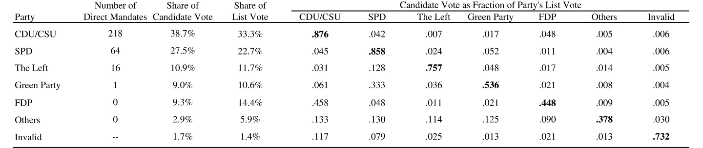
Before doing so, however, it is useful to get a sense of the broad patterns in the data. Table 1 shows aggregate frequencies of di erent list and candidate vote combinations in the 2009 federal election.8 First and foremost, the evidence suggests that some, but not
all, voters desert weak candidates. Although nominees of FDP, Greens, and other minor parties are rarely in contention for victory, they are abandoned by only about half of their followers. At the same time, the numbers show that, conditional on abandoning their own party's candidate, about 83% of all FDP supporters voted for a contestant of the CDU| its coalition partner|whereas 72% of Green Party adherents chose an SPD nominee. It, therefore, appears that voters who do desert noncontenders substitute toward close political
8
allies.
Although Table 1 is suggestive of some voters behaving strategically, with others likely being sincere, it is ultimately insu cient to quantify the prevalence of either type of behavior. Again, some FDP supporters might have chosen CDU candidates not because of tactical considerations, but because they are better quali ed or more charismatic. Also, not all CDU and SPD adherents voted for their own party's nominee. In fact, almost one-third of those who deviate end up picking a political rival. While it is possible that these voters chose among the lesser of two evils in districts in which the CDU or the SPD candidate happened to be \out of the race," it is also plausible that their voting decisions were based on candidate idiosyncrasies.
In fact, the descriptive statistics in Table 2A demonstrate that candidates di er along several dimensions.9 For instance, only 19% of CDU candidates are female, compared with
35% of Social Democrats and 34% of Green Party nominees. 95% of SPD candidates are also on the party list, compared with 43% of their colleagues from The Left. Moreover, relative to their FDP, Left, or Green Party counterparts, CDU and SPD contestants are about four times more likely to be a current member of parliament and more than forty times as likely to be an incumbent. Therefore, any argument linking di erences in the distribution of list and candidate votes to (ir)rational behavior must be based on an econometric strategy that carefully controls for candidates' idiosyncratic appeal.
To this end, the present paper relies on o cial results of the 2005 and 2009 federal elec-tions, by polling precinct (Wahlbezirk).10 These data have been obtained from the Federal
Returning O cer and were until recently not publicly available. In Germany, precincts are the smallest administrative units in which votes are counted. Each precinct is fully contained within an electoral district and associated with one polling station where a returning o -cer oversees the election. By law, no precinct can contain more than 2,500 eligible voters. As of 2009, there were 299 electoral districts and almost 89,000 precincts. Since races take place at the level of the electoral district, precinct-level data allow for all estimates to be based on within-candidate variation only, thereby conditioning on all observable as well as unobservable characteristics of candidates and their competitors, the marginal candidates on parties' lists, pivot probabilities, and many other sources of unobserved heterogeneity across
9
The information in Table 2A has been compiled from o cial publications by the Federal Returning O cer (Bundeswahlleiter 2005c, 2009b).
10
candidates and districts.
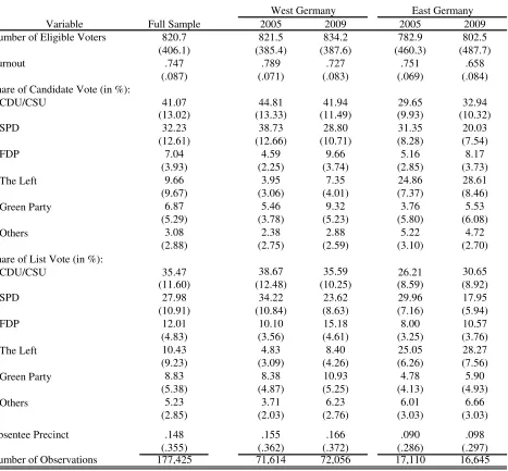
Di erentiating between East and West Germany as well as election year, Table 2B dis-plays summary statistics for all precinct-level variables. Compared with the U.S., turnout is fairly high. Averaging across 2005 and 2009, almost 75% of the electorate went to the polls. Together with an average size of 821 eligible voters, this means that precincts handle about 615 votes. As is well-known, CDU, SPD, FDP, and the Green Party fare substantially better in West Germany than in the East. The opposite is true for The Left. Moreover, CDU and SPD receive more candidate than list votes. Given that the nominees of these two parties are serious contenders in most districts, this could, but need not, be due to strategic voting.
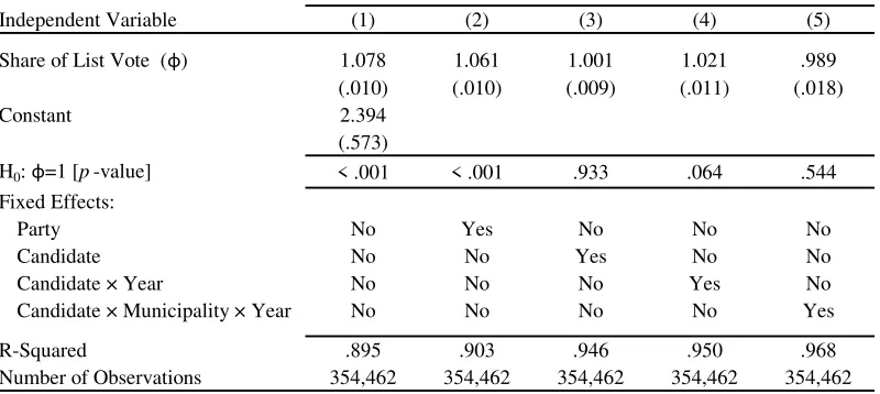
3.2. Testing the Null Hypothesis of Sincere Voting
Following the argument in the introduction, it is straightforward to test the null hypothesis that voters are \behavioral" in the sense that they fail to internalize the electoral incentives. If, as in a substantial part of the theoretical literature, all individuals simply choose their most preferred option|meaning that they cast sincere listand sincere candidate votes|and if preferences over parties are su ciently correlated with that over candidates, then, after carefully controlling for nominees' idiosyncratic appeal, it should be the case that list and candidate vote shares track each other almost one for one. That is, under the null hypothesis of sincere voting, an extra list vote should translate into an additional vote for the nominee of the respective party.
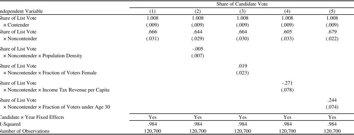
The results in the upper panel of Table 3 show that this is not the case. The ordinary least squares estimates therein correspond to the econometric model
(1) vk;r;tC = m;k;t+ vLk;r;t+ k;r;t;
where vC
k;r;t denotes contestant k's share of the candidate vote in precinct r during election year t, and vL
k;r;t is her party's share of the list vote in the same precinct. To allow for ar-bitrary forms of autocorrelation in the residuals as well as for correlation within and across districts, standard errors are clustered by state.11 Going from the left of the table to the
right, the set of xed e ects grows steadily. The most inclusive speci cation contains m;k;t, a municipality- and year-speci c candidate xed e ect. It, therefore, controls nonparametri-cally for the appeal of individual candidates (and that of their competitors) as perceived by the voters in a given town or village.12
11
Note that there are only 16 states in Germany, which raises issues associated with a small number of clusters. In order to account for this issue when testing hypotheses, the reportedp-values are based on the wild bootstrap procedure suggested by Cameron et al. (2008).
12
munic-Using this model, one can dismiss the null of sincere voting if it is possible to reject
H0 : = 1. Clearly, in all speci cations of Table 3 that control for candidates' idiosyncrasies,
the slope between list and candidate votes is considerably smaller than one (p < :001). On average, only nine out of ten voters stick with the same party's candidate. Put di erently, for about 10% of agents observed choices are inconsistent with sincere behavior.
Of course, all hypothesis tests are joint tests of the null and the underlying assumptions. Under the null hypothesis, list and candidate votes must reveal voters' true preferences over parties and candidates, respectively. The actual identifying assumption then is not that list votes proxy for preferences, but that tastes for parties and candidates are heavily correlated, at least after strongly controlling for candidate quality. This assumption is testable.
To see that is does appear to hold, consider the lower two panels in Table 3. The middle one restricts attention to the eventual winner and runner-up of each race. Voters who support the parties associated with these candidates have no strategic reason to cast split ballots. After all, surprises in large-scale elections are very rare, and partisans have no incentive to desert someone they should have believed to be in contention for victory. Thus, if party votes are, indeed, heavily correlated with individuals' preferences over candidates, then, in this subsample of the data, party and candidate vote shares ought to track each other very closely. Conversely, seeing a slope considerably smaller than unity should lead one to question the identifying assumption.
Fortunately, there is no indication that this is warranted. After accounting for candidate quality, candidate and list vote shares move together almost one for one. Taking the estimate in column (5) at face value, it appears that, on the margin, an extra list vote results in about
:989 additional candidate votes. Although the point estimate is quite precise, it isnot possible to rule out that it is exactly equal to one.13
By contrast, the bottom panel focuses on candidates who nished in third place or worse. At least some agents who voted for the parties associated with these candidates had a strategic incentive to cast split ballots; and about one in three did so. Taken together, the results in Table 3 reject the null hypothesis that all voters are \behavioral."
4. Quantifying Deviations from Instrumental Rationality
4.1. Econometric Approach
Strictly speaking, the evidence thus far only shows that observed choices are incompatible with sincere behavior for about 10% of voters. It does not rule out that most agents are
ipalities. This allows for straightforward identi cation of m;k;t.
13
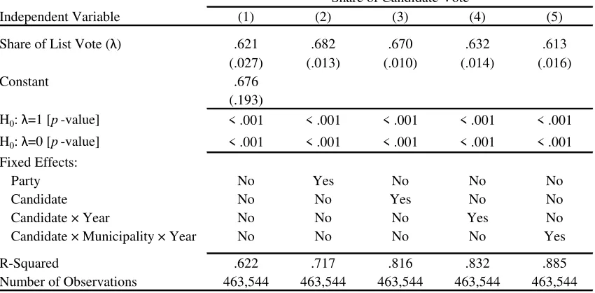
strategic but happen to cast ballots that are also consistent with sincerity. In order to shed light on how frequently the predictions of canonical rational choice theory are actually violated, and to inform our understanding of the extent to which individuals behave \as if" they are unboundedly rational, this section pursues two related empirical strategies.
The rst strategy identi es the share of voters whose choices deviate from instrumental rationality by considering only candidates who were clearly not in contention for victory. This approach's main requirement is that, conditional on the equilibrium being observed by the econometrician, one can nd a subset of nominees whom rational voters cannot have believed to be \in the race." For this set of candidates, one then estimates
(2) vk;r;tC = m;k;t+ vk;r;tL + k;r;t;
where all symbols are as de ned above.14
The parameter of interest is . It denotes the fraction of party supporters who stick with the associated candidate despite her being \out of the race." As explained at the end of Section 2, the share of agents whose observed choices violate the canonical pivotal voter model is a lower bound on the actual fraction of noninstrumentally rational voters. The reason is that, without observing individuals' true preferences, some choices will appear consistent with instrumental rationality, even though agents were not strategically motivated.
Thus, one reason to control for candidate quality by including municipality- and year-speci c candidate xed e ects, i.e. m;k;t, is to tighten the estimated bound. The more important reason, however, is to ensure that can, in fact, be interpreted as a lower bound. In the absence of individual-level data on vote combinations, there remains the possibility that candidatekreceived a substantial share of her votes from the supporters of other parties. Although the behavior of these individuals is also inconsistent with instrumental rationality, simply dividing the number of candidate votes by the number of party votes might lead to an overestimate of the share of behavioral agents|in extreme cases this ratio might even exceed one. It is, therefore, preferable to explicitly control for candidate quality and estimate at the margin. That is, is identi ed from changes in candidates' vote shares as a result of cross-precinct variation in the vote shares of the associated parties.15
Of course, if one were willing to assume that list votes are a good proxy for voters' (induced) preferences over candidates, then most of these issues would become moot. In the ideal case
14
It is straightforward to derive equation (2) from a simple model along the lines of Myerson and Weber (1993), extended to include a sincere type of voter (see Spenkuch 2013).
15
in which preferences over parties and candidates are perfectly correlated, would exactly identify the fraction of voters who fail to abandon their prefered candidate despite her being out of the race. While the evidence in the middle panel of Table 3 suggests that such an assumption may not be completely unreasonable|especially after carefully controlling for candidates' idiosyncrasies|it is important to emphasize that it isnot required. Without it, the point estimates still recover a lower bound on the share of behavioral agents.
Also note that, as long as there is no heterogeneity in , it is irrelevant if the set of candidates who are included in the sample used to estimate equation (2) is chosen too conservatively, i.e. if one discards some candidates who were also believed to be \out of the race." Settling on a too narrowly de ned set of noncontenders would only come at a loss of statistical power, but it would not prevent consistent estimation of .
If, however, there is heterogeneity in and if this heterogeneity is systematically correlated with who remains in contention for victory, then restricting attention to supporters of parties that eld candidates who trail far behind might lead to biased estimates. The second (and, therefore, preferred) empirical strategy addresses this problem by adopting a data-driven approach to classifying contestants.16
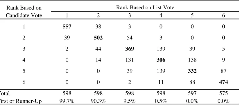
To see that the actual data are highly predictive of which candidates end up competing for a direct mandate, consider Table 4, which shows a cross-tabulation of candidates' own rank (based on the candidate vote) against the standing of their party among voters in the same district (based on the list vote). Out of the 598 contestants whose party placed rst, only 41 did not win a direct mandate, and a mere 2 nished third or worse. In contrast, none of the candidates who ran for a party ranked fourth or below came in rst, and only 3 nished second. Overall, the correlation between list and candidate vote based rank is :93. The evidence, therefore, suggests that voters coordinate on the nominees of the district's most popular parties.
If one believes that agents do, indeed, play focal equilibria of this type, then contestants backed by one of a district's two favored parties should be considered serious contenders, whereas candidates of parties ranked fourth and below are \out of the race." The only ambiguity arises with respect to those in third place. In practice, almost 10% of third ranked contestants nish rst or second. Hence, one would want to classify some (but not all) of them as contenders, especially in cases in which only a few percentage points separate their own party from the one in second place.17
16
Unfortunately, pre-election surveys in Germany are too small to derive reliable estimates of voters' expec-tations. For instance, in only 50 electoral districts did the German Longitudinal Election Study (GLES)|the best available data source|survey more than 15 adults prior to the 2009 elections.
17
Drawing from the literature on structural breaks in time series data, it is possible to estimate a cuto value, , separating candidates into contenders and noncontenders. More speci cally, the second empirical strategy classi es candidatek as a contender if, and only if, her party trails a district's second most popular candidate by less than percentage points.
With this de nition in hand, the estimating equation becomes
(3) vCk;r;t= m;k;t+ vLk;r;t 1
h
vL;d;t2nd v L k;d;t >
i
+ vLk;r;t 1
h
vL;d;t2nd v L k;d;t
i
+ k;r;t:
Here, vL
k;d;t denotes the list vote share of candidate k's party in districtd, and v L;2nd
d;t is that of the second most popular party in the same district.
If (3) is correctly speci ed, then searching for the value of that maximizes the R2 yields
a super-consistent estimate of the true break point (Hansen 2000). Moreover, under the null hypothesis that such a point exists, estimates of the model's other parameters are normally distributed, and standard errors need not be adjusted for sampling variability in the location of the break (see, e.g., Bai 1997).
Although intuitively appealing, there is no guarantee that this method classi es all candi-dates correctly. For this reason, Section 4.4 performs a series of robustness checks, demon-strating that the main results are qualitatively and quantitatively robust to more than 25 alternative assumptions on how voters form beliefs about which candidates are in contention for victory.
4.2. Main Results
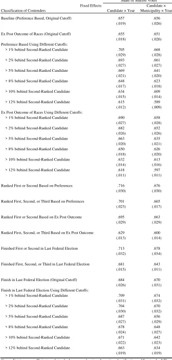
Focusing on nominees of the ve major parties, Table 5 displays the main results. The upper panel follows the rst empirical strategy and restricts the sample to candidates who trailed the runner-up by more than 10 percentage points. The lower panel implements the second approach.
The rst row within each panel presents estimates of the share of behavioral voters, i.e. those who stick with a party's candidate despite her having no chance of winning. Controlling for the idiosyncrasies of candidates and their competitors, estimates of range from :613 to
:657 and are fairly precise. Moreover, it is worth noting that the evidence from both empirical approaches lines up very well. Despite small standard errors, estimates from the rst and second approaches are statistically indistinguishable. Taken at face value, the results indicate that (at least) 65% of voters do not behave in accordance with the canonical rational choice model.
An important question is whether most agents who do cast split ballots when it is optimal
to do so are, in fact, strategically motivated. Strictly speaking, any model that predicts the candidate{list vote gradient for noncontenders to lie between zero and one is consistent with the evidence presented in Table 5. For instance, some fraction of individuals might simply vote for whichever candidate advertises the most, and advertising expenditures may be highly correlated with who remains in contention for victory. It would, therefore, appear as if some voters abandon weak candidates, despite the fact that most agents do not behave tactically. In such a case, the estimates above might severely understate the extent of \behavioral" voting.
In order to rule out mechanical explanations of this kind, Table 6 compares estimates of across a number of di erent settings. The rst set of results demonstrates that the extent to which observed behavior violates instrumental rationality depends on who remains in contention for victory. That is, conditional on voting for a party whose candidate is \out of the race," agents are about 25 percentage points less likely to stick with a noncontestant when the candidate of an allied party is still \in the race" than when faced with the choice among two evils, i.e. less palatable alternatives.18 A Chow test for equality of coe cients
rejects the null hypothesis of equal point estimates at the 1%-level.
Moreover, distinguishing between races that were \close" and those that were not, sincere voting appears to have been less prevalent in the former|though the di erence is not sta-tistically signi cant|and disaggregating the data by election year shows that desertion of noncontenders was signi cantly more common in 2005 than in 2009 (p < :001).
This is not surprising. The 2005 election followed a failed motion of con dence that trig-gered the dissolution of the Bundestag and was widely perceived to be a \critical election," in which di erences between parties and, therefore, the stakes were signi cantly higher than usual (Korte 2009).19 In line with these results, o cial statistics show a substantially larger
fraction of split tickets in 2005, and an approximately 7 percentage points higher turnout than in 2009 (Bundeswahlleiter 2006, 2010).
The change in turnout, however, is too small to account for the entire di erence in . Estimating the share of behavioral voters for each municipality-year combination separately and regressing the resulting k;t on turnout in the respective village in the same year yields a point estimate of :698 (with a standard error of:173). Based on this evidence, a 7 percentage point increase in turnout would be predicted to lead to an approximately 4:9 percentage
18
The following parties are de ned as allies: CDU and FDP, SPD and Green Party. Results are qualitatively similar if supporters of The Left are assumed to consider SPD candidates to be close substitutes. Also, note that there were no uncontested races in 2005 and 2009.
19
points lower fraction of behavioral voters. While the available evidence does suggest that inframarginal voters are considerably more likely to violate instrumental rationality than marginal ones, a 7 percentage point increase in turnout would not cause a near 50% change in the estimated extent of sincere voting. Some simple back-of-the-envelope calculations show that this conclusion continues to hold even if every additional voter is assumed to behave strategically.20
Importantly, the results in Table 6 are at odds with many mechanical theories for why voters abandon candidates who are \out of the race." Any model in which voters desert candidates for nonstrategic reasons would not only have to predict a correlation between desertion rates and a contestant's chance of winning, but it would also have to explain why defection is more common among marginal voters, when the stakes are higher, and why it depends on which candidates remain in contention for victory. The patterns above, as well as the fact that voters who do cast split tickets substitute toward candidates of a potential coalition partner (cf. Table 1), suggests that desertion is, in fact, driven by instrumentally rational considerations.
4.3. Interpreting the Evidence
Neither the canonical rational choice model nor behavioral theories in which agents simply vote for their favorite candidates are able to explain the ndings above. Instead, the evidence suggests that it might be more appropriate to consider strategic behavior a conscious decision rather than an agent's \type." That is, all agents may be capable of voting tactically, but only for a subset of them do the subjective bene ts outweigh the (psychic) costs of abandoning the candidate of one's preferred party or of guring out one's optimal strategy. In such a richer model, would not refer to the population share of behavioral \types," but to the fraction of voters whose costs are below some endogenously determined threshold.21
If a large share of voters have costs very close, but not exactly equal, to zero, then such a hybrid model with boundedly rational agents would predict the two most-salient features of the data: (i) most voters do not ( nd it worthwhile to) abandon weak candidates, but (ii) when the stakes increase, agents' tendency to \waste their vote" plummets. That is, a
20
In 2005, about 13.3 million voters chose a party whose direct candidate is estimated to be \out of the race," and almost half of them also abandoned the respective nominees. Suppose that every single one of the approximately 4 million additional voters in 2005 chose a party whose direct candidate was not in contention for victory and deserted the respective direct candidate. If this were, indeed, the case, then about 70% of the inframarginal voters, i.e. 6.5 out of 9.3 million, would not have behaved instrumentally rational. Even under these extreme assumptions, the di erence in turnout cannot account for only the entire change in .
21
signi cant share of agents are close enough to the margin, so that small changes in absolute payo s cause large shifts in observed behavior.
Another potential explanation for the preceding ndings is that individuals receive a het-erogeneously distributed utility boost from voting for the eventual winner of the election. If the utility bene t from doing so was close, but not exactly equal, to zero for su ciently many agents, then such a model of \bandwagon e ects" (Simon 1954) would be able to rationalize (i). Moreover, if the bene t of voting for the winner depends on the perceived stakes of the election, then bandwagon e ects might also be consistent with (ii).
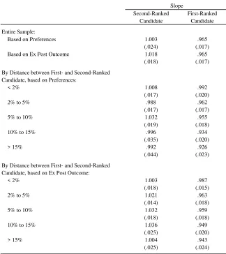
The key testable di erence between both theories is that the latter predicts runner-ups to be abandoned as well, especially those who trail far behind and are, therefore, unlikely to win. By contrast, a pivotal voter model in which agents face a cost from behaving strategically predicts that agents do not abandon the runner-up, even if her chances of winning are very small. This is because if a race were to be tied|however unlikely that may be|the tie would almost certainly involve the second-ranked candidate (see Myerson 2000, 2002; Myerson and Weber 1993), in which case voting for her would change the outcome of the election. Thus, even agents who choose to cast tactical ballots would not abandon a runner-up who trails far behind.
Although counterintuitive, the evidence in Table 7 supports this prediction. The numbers therein refer to the slope parameter, i.e. in equation (1), estimated separately for rst-and second-ranked crst-andidates, by distance between the two. Perhaps surprisingly, all point estimates are rather close to one, and, if anything, the coe cients for second-ranked candi-dates are slightly larger than those for their rst-ranked counterparts. This helps to rule out alternative explanations based on bandwagon e ects.
4.4. Sensitivity and Robustness Checks
of Table 5.
Although individual point estimates do, of course, vary, the majority of them are very close to their baseline values. For instance, assuming that voters have perfect foresight regarding the winner and runner-up of the election, one would estimate the fraction of behavioral votes to equal 66:3% instead of 65:6%, whereas adaptive expectations based on the outcome of the last election (i.e. the winner and runner-up in the previous federal election are believed to be \in the race") would lead to point estimates ranging from 67:8% to 71:3%. Of the fty-two additional estimates in Table 8, the lowest one is 58:9% and the highest one equals 71:6%. Slightly more than 90% of coe cients fall within the original 95%-con dence intervals. The evidence, therefore, suggests that misclassi cation of contestants is not a rst-order problem.
Exact Indi erence Some individuals could beexactly indi erent about who carries their district, and might therefore stick with a candidate who is \out of the race." The empirical strategy in this paper would classify these agents as \behavioral," leading to estimates of that include indi erent voters.
One piece of evidence suggesting that the vast majority of voters are not indi erent to who represents them in parliament comes from the fact that less than 2% of those going to the polls cast invalid or no candidate votes (despite the fact that it is possible to cast a valid list vote while leaving the candidate vote blank). For the U.S., for instance, it has been argued that ballot roll-o (i.e. voters not completing one of several sections on the ballot) is a sign of voters not caring \enough" about a particular race (e.g., Bullock and Dunn 1996; Burnham 1965). If Germans were exactly indi erent about district-level races, then one would not expect them to be willing to incur even a small \hassle cost" to cast their candidate vote. The fact that more than 98% of voters do cast valid candidate votes suggests that the potential bias from exact indi erence is likely very small.
Endogenous Nomination of Candidates Another concern relates to the behavior of parties. Depending on the anticipated likelihood of winning the district, parties might nomi-nate a particularly \good" or \bad" candidate. Since the empirical strategy relies on within-candidate variation, this sort of behavior could bias the point estimates if within-candidate quality interacts with the share of voters who choose to behave sincerely|say, because voters might be reluctant to abandon very charismatic contestants. Although plausible, the data do not suggest that \good" candidates, as measured by k;t, are less likely to be deserted when they are \out of the race." If anything, estimating separate slope parameters for all candidate-year combinations and regressing them on the estimated xed e ects shows that the covariance between k;t and a noncontender's k;t is slightly negative.
have more supporters and that this may lead to bias in . However, estimating for each candidate-year combination and regressing the resulting k;t on the district-wide list vote as a measure of party strength yields a point estimate of :001 with a standard error of :003, which is not only economically small but also statistically indistinguishable from zero. Put di erently, local party strength is nearly uncorrelated with the estimated share of voters who stick with the respective candidate.
To get a sense of how varies with candidates' observational characteristics, consider Appendix Table A.2. Although voters appear to desert younger candidates somewhat more frequently than older ones, the point estimates have a very similar range as those in Table 8, which suggests that there is no single type of candidate that drives the results. That is, even if one were to focus on the types of candidates delivering the most-extreme estimates, one would still conclude that neither the pivotal voter model nor a theory based on sincere voting provides an accurate description of reality.
Also note that the results cannot be driven by comparisons between direct candidates and those on the party list. While it is theoretically possible that some agents desert their favorite party's candidate because they would like someone else on the party list to enter parliament instead (see Section 2 or Appendix A for details on how seats are allocated), this behavior should not a ect the estimates. The reason is simple. None of the identifying variation comes from candidates who are in contention for victory, i.e. who have a realistic chance of entering the Bundestag and for whom this sort of comparison is theoretically relevant. Moreover, whatever voters may think about the marginal candidates on parties' lists, it continues to be true that voting for someone who is not in contention for victory will not a ect the outcome of the election and is, therefore, inconsistent with the predictions of the pivotal voter model.
Additional Robustness Checks The remainder of Table 9 demonstrates that the results do not depend on the weighting scheme nor on whether one also includes candidates of \micro parties."
5. Observed Violations of Instrumental Rationality and Voter Characteristics
The evidence above shows that a nontrivial fraction of agents does not behave as predicted by standard theories of voting. Though it does appear that the share of voters whose behavior violates canonical rational choice decreases with the electoral stakes, most agents just stick with weak candidates. Simple averages, however, may conceal considerable heterogeneity across individuals, which is why it is also important to understandwhovotes \behaviorally." In order to infer whether varies with the characteristics of the electorate, the present paper relies on o cial statistics for the universe of German cities and villages, published by the Federal Statistical O ce and the statistical o ces of the L•ander (Statistische •Amter des Bundes und der L•ander 2007, 2011).22 After aggregating election results to the village level
and focusing on the set of municipalities that are fully contained within an electoral district, it is straightforward to estimate speci cations that allow for to increase or decrease in some village characteristic.
Table 10 displays the results. The rst column demonstrates that aggregation to the mu-nicipality level does not materially a ect the point estimates. The remaining four columns examine how changes with population density, income tax revenue per capita, as well as the gender and age composition of the electorate. For ease of interpretation, covariates have been demeaned, so that the estimates in the second row refer to the share of behavioral voters at the sample average.
Interestingly, urban voters are not less behavioral than rural ones, nor is there a signi cant gender gap. The results do, however, indicate di erences with respect to socioeconomic status (as proxied by income tax revenue per capita) and age.
Since the income tax variable captures only revenues that accrue to the respective munici-palities, and given that the German tax system is highly nonlinear, it is easiest to judge the magnitude of the coe cient by an example. Consider two villages: one's per capita income tax revenue is a standard deviation below the mean, while that of the other village is one standard deviation above the sample average.23 The share of voters who do not abandon a
weak candidate is estimated to be almost 6 percentage points lower in the latter.
Disparities by age are even larger. Taken at face value, the coe cient in column (5) suggests
22
Unfortunately, comparable data for polling precincts do not exist. Polling precincts are too small to produce reliable estimates from existing data sets.
23
that observed violations of the pivotal voter model are almost universal among voters below the age of 30, i.e. those who could have participated in, at most, three federal elections. Of course, the respective estimate is based on limited variation and is therefore not very precise. But, together with the results in column (4), it suggests that sophistication and experience correlate with the extent to which agents act in accordance with traditional rational choice theory.
To further investigate the e ect of experience, the remainder of this section uses the Ger-man Reuni cation as a natural experiment. Although the GerGer-man Democratic Republic (GDR) held regular, formal elections to the Volkskammer (People's Chamber), they were e ectively meaningless. East Germans could only choose from candidates on a single list controlled by the Socialist Unity Party (SED), and it was customary to cast one's ballot in public, simply accepting all nominated candidates. Unsurprisingly, o cial approval rates often exceeded 99%. Free, democratic elections were only held on March 18, 1990|after months of peaceful political protest. The newly elected government then negotiated the end of the GDR.
In stark contrast, citizens of the Federal Republic of Germany had the opportunity to participate in free elections since 1949, and, from 1953 on, under a two-ballot system almost identical to the current one. Thus, they had more than 40 years of democratic experience by the time the GDR joined the West.
The rst parliamentary elections in uni ed Germany were held on December 2, 1990 and were subject to (essentially) the same rules that had previously been used in the West and that continue to be in place today.24 If experience and familiarity with the electoral system
do indeed matter, then one would expect large initial di erences in the share of agents whose behavior is at odds with instrumental rationality, which should disappear over time.
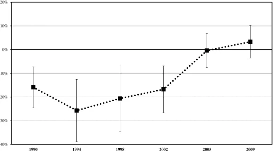
This prediction is borne out in Figure 2. For each election since 1990, the gure plots the estimated di erence in the share of behavioral voters between East and West Germany. Negative values indicate more violations of the pivotal voter model among residents of the former GDR.25
The results show that just two months after reuni cation, East Germans were almost 16 percentage points more likely to stick with a noncontender than their Western counterparts. By 2005, however, the gap had vanished. Although none of the point estimates is very precise,
24
The most important exception was that the 5%-threshold applied separately to East and West Germany. Thus, in 1990 a party had to gain more than 5% of the list vote in only one of the two regions to enter the Bundestag.
25
one can nevertheless reject the null hypothesis of a constant di erence at the 1%-signi cance level. Moreover, both the initial gap as well as the speed of convergence are in line with the \age e ect" in Table 10.26
6. Related Literature
There exists a large empirical literature concerned with the extent of instrumental ratio-nality in voting. Within this literature, laboratory experiments provide typically convincing evidence of tactical behavior by some, but not all, individuals (e.g., Du y and Tavits 2008; Eckel and Holt 1989; Esponda and Vespa 2013). Interestingly, the share of strategic agents generally increases with subjects' experience and the availability of coordination devices, such as pre-election polls (e.g., Forsythe et al. 1993, 1996). However, given the relatively small number of subjects in the laboratory, it remains unknown whether these results generalize to large, real-world elections.
The evidence on this question is decidedly mixed. Coate et al. (2008), for instance, reject the pivotal voter model based on the nding that it is unable to replicate winning margins in Texas liquor referenda. Reed (1990) and Cox (1994), however, argue that the distribution of votes in Japan's multimember districts does conform to the predictions of rational choice theory. More recently, Fujiwara (2011) uses a sharp regression discontinuity in Brazilian mayoral elections to show that third-place candidates are more likely to be deserted in races under simple plurality rule than in runo elections. The most comprehensive study to date is Cox (1997). His ndings are suggestive of strategic behavior in a number of electoral systems but indicate a lack thereof in others.
Even less is known about theextent of instrumental rationality among voters, or violations thereof. Two recent exceptions are Spenkuch (2014) as well as Kawai and Watanabe (2013). Spenkuch (2014) exploits a highly unusual by-election in Germany, which allowed a party to gain one seat by receiving fewer votes, to show that at least 9% of voters did not behave sincerely.
Kawai and Watanabe (2013) estimate a fully structural model of voting decisions in Japan's general election, concluding that between 63% and 85% of voters are strategic|but in equi-librium less than 5% cast misaligned votes. Put di erently, Kawai and Watanabe (2013) estimate that, at most, 37% of Japanese voters are sincere, whereas this paper derives a lower bound of about 65%. Whether this discrepancy is due to systematic di erences in the environment (say, higher stakes in Japanese elections), true di erences in the rationality
26
of the underlying populations, or di erences in the empirical approach is (as of yet) un-known. Although Japan uses a mixed-member electoral system similar to the German one, it is important to note that the analysis in Kawai and Watanabe (2013) makes no use of party votes. All identi cation comes from variation in candidate vote shares and observable characterictics of voters.
Recall, the fundamental di culty in inferring (non)strategic behavior from naturally oc-curring data is that voters' preferences are not observed. Thus, any existing evidence is either based on indirect tests (as in Coate et al. 2008; Cox 1997; Fujiwara 2011; Spenkuch 2014), or preference orderings are structurally estimated in order to compare them to actual vote counts (as in Kawai and Watanabe 2013).
A separate strand of the literature tries to circumvent these problems by using survey data on voting decisions and political orientations (see, e.g., Abramson et al. 1992; Blais et al. 2001; Kiewiet 2013; Niemi et al. 1993; or, for Germany, Gschwend 2007; Pappi and Thurner 2002). Estimates in this tradition are often very low. Wright (1990, 1992), however, points to important survey biases and raises serious doubts about conclusions based on self-reported votes. Alvarez and Nagler (2000) even show that, depending on the survey design, estimates of instrumentally rational voting di er by as much as a factor of seven.
7. Concluding Remarks
Whether individuals act approximately \as if" they are unboundedly rational is an important question in economics. In the context of social choice it has interested scholars for more than six decades. Yet, outside of the laboratory it has proven extremely di cult to quantify deviations from the baseline pivotal voter model. By exploiting the incentive structure of parliamentary elections in Germany, the present paper presents evidence indicating that at least 65% of voters do not behave as predicted by standard rational choice theory.
Of course, in light of a plethora of anecdotal evidence, one might not have expected literally all agents to be \perfectly rational," especially not in large elections with arguably weak electoral incentives. Nevertheless, the results above are noteworthy for at least two reasons. First, the magnitude of the point estimates implies that the single most common assumption about the behavior of voters is violated for the vast majority of agents. Second, the leading alternative theory according to which voters sincerely choose their most preferred candidate is also rejected by the data.
agents pay a \psychic" cost to behave strategically, the results suggest that a signi cant number of people face very low costs and are thus close to the margin of acting strategically.
References
Alesina, A., andH. Rosenthal(1996). \A Theory of Divided Government."Econometrica, 64, 1311{1341.
Abramson, P. R.,J. H. Aldrich,P. Paolino, andD. W. Rohde(1992). \Sophisticated Voting in the 1988 Presidential Primaries,"American Political Science Review, 86, 55{69.
Alvarez, R. M., and J. Nagler(2000). \A New Approach for Modelling Strategic Voting in Multiparty Elections."British Journal of Political Science, 30, 57{75.
Arrow, K. J.(1951).Social Choice and Individual Values.New York: Wiley.
Austen-Smith, D., andJ. S. Banks(1988). \Elections, Coalitions, and Legislative Outcomes."American
Political Science Review, 82, 405{422.
Bai, J. (1997). \Estimation of a Change Point in Multiple Regression Models." Review of Economics and
Statistics, 79, 551{563.
Barbera, S. (2011). \Strategyproof Social Choice," (pp. 731{831) in K. J. Arrow, A. K. Sen, and K. Suzumaru(eds.),Handbook of Social Choice and Welfare, Vol. 2. Amsterdam: Elsevier.
Becker, G. S. (1993). \Nobel Lecture: The Economic Way of Looking at Behavior." Journal of Political
Economy, 101, 385{409.
Benjamin, D. J., S. A. Brown, andJ. M. Shapiro(2013). \Who is Behavioral? Cognitive Ability and Anomalous Preferences."Journal of the European Economic Association, 11, 1231{1255.
Besley, T., andS. Coate(1997). \An Economic Model of Representative Democracy."Quarterly Journal
of Economics, 112, 85{114.
Black, D.(1948). \On the Rationale of Group Decision-making."Journal of Political Economy, 56, 23{34.
Blais, A.,R. Nadeau,E. Gidengil, andN. Nevitte(2001). \Measuring Strategic Voting in Multiparty Elections."Electoral Studies, 20, 343{352.
Bouton, L. (2013) \A Theory of Strategic Voting in Runo Elections."American Economic Review, 103, 1248-1288
Bundeswahlleiter (2005a). Wahl zum 16. Deutschen Bundestag am 18. September 2005. Heft 3:
Endg•ultige Ergebnisse nach Wahlkreisen. Wiesbaden: Statistisches Bundesamt.
(2005b).Wahlkreiskarte f•ur die Wahl zum 16. Deutschen Bundestag. Wiesbaden: Statistisches Bun-desamt.
(2005c).Wahl zum 16. Deutschen Bundestag am 18. September 2005. Sonderheft: Die Wahlbewerber
f•ur die Wahl zum 16. Deutschen Bundestag 2005. Wiesbaden: Statistisches Bundesamt.
(2006).Wahl zum 16. Deutschen Bundestag am 18. September 2005. Heft 4: Wahlbeteiligung und
Stimmabgabe der M•anner und Frauen nach Altersgruppen. Wiesbaden: Statistisches Bundesamt.
(2008).Wahlkreiskarte f•ur die Wahl zum 17. Deutschen Bundestag. Wiesbaden: Statistisches Bun-desamt.
(2009a).Wahl zum 17. Deutschen Bundestag am 27. September 2009. Heft 3: Endg•ultige Ergebnisse
nach Wahlkreisen. Wiesbaden: Statistisches Bundesamt.
(2009b).Wahl zum 17. Deutschen Bundestag am 27. September 2009. Sonderheft: Die Wahlbewerber
f•ur die Wahl zum 17. Deutschen Bundestag 2009. Wiesbaden: Statistisches Bundesamt.
(2010).Wahl zum 17. Deutschen Bundestag am 27. September 2009. Heft 4: Wahlbeteiligung und
Bullock, C. S., andR. E. Dunn(1996). \Election Roll-O : A Test of Three Explanations."Urban A airs
Review,32, 71{86.
Burnham, W. D. (1965). \The Changing Shape of the American Political Universe." American Political
Science Review, 59, 7{28.
Callander, S. (2005) \Electoral competition in heterogeneous districts." Journal of Political Economy, 113, 1116{1145.
Camerer, C.(2006). \Behavioral Economics," (pp. 181{214) inR. Blundell,W. Newey, andT. Pers-son(eds.),Advances in Economics and Econometrics: Theory and Applications, Ninth World Congress,
Vol. 2. Cambridge, UK: Cambridge University Press.
Cameron, A. C.,J. B. Gelbach, andD. L. Miller(2008). \Bootstrap-based Improvements for Inference with Clustered Errors."Review of Economics and Statistics, 90, 414{427.
Choi, S., S. Kariv, W. M•uller, and D. Silverman(2014).\Who Is (More) Rational?"American
Eco-nomic Review, 104, 1518-50.
Coate, S., M. Conlin, andA. Moro(2008). \The Performance of Pivotal-Voter Models in Small-Scale Elections: Evidence from Texas Liquor Referenda."Journal of Public Economics, 92, 582{596.
Conlisk, J.(1996). \Why Bounded Rationality?"Journal of Economic Literature, 34, 669{700.
Cox, G. W.(1994). \Strategic Voting Equilibria Under the Single Nontransferable Vote."American Political
Science Review, 88, 608{621.
(1997).Making Votes Count. Cambridge, UK: Cambridge University Press.
Degan, A., and A. Merlo (2009). \Do Voters Vote Ideologically?" Journal of Economic Theory, 144, 1868{1894.
DellaVigna, S. (2009). \Psychology and Economics: Evidence from the Field." Journal of Economic
Literature, 47, 315{72.
, J. A. List, U. Malmendier,andG. Rao(2013). \Voting to Tell Others." NBER Working Paper No. 19832.
Downs, A.(1957).An Economic Theory of Democracy. New York: Harper & Row.
Duverger, M.(1954).Political Parties: Their Organization and Activity in the Modern State. New York: Wiley.
Duffy, J., and M. Tavits (2008). \Beliefs and Voting Decisions: A Test of the Pivotal Voter Model."
American Journal of Political Science, 52, 603{618.
Eckel, C., and C. A. Holt (1989). \Strategic Voting in Agenda-Controlled Experiments." American
Economic Review, 79, 763{773.
Esponda, I., andE. Vespa(2013). \Hypothetical Thinking and Information Extraction in the Laboratory."
American Economic Journal: Microeconomics, forthcoming.
Farquharson, R.(1969).Theory of Voting. Oxford: Blackwell.
Feddersen, T. J., andW. Pesendorfer(1996). \The Swing Voter's Curse."American Economic Review, 86, 408{424.
Forsythe, R.,R. B. Myerson,T. A. Rietz, andR. J. Weber(1993). \An Experiment on Coordination in Multi-Candidate Elections: The Importance of Polls and Election Histories."Social Choice and Welfare, 10, 223{247.
, T. A. Rietz, R. B. Myerson, and R. J. Weber (1996). \An Experimental Study of Voting Rules and Polls in Three-Candidate Elections."International Journal of Game Theory, 25, 355{383.
Journal of Political Science, 6, 197{233.
Gibbard, A.(1973). \Manipulation of Voting Schemes: A General Result."Econometrica, 41, 587{601.
Green, D. P., andI. Shapiro (1994).Pathologies of Rational Choice Theory: A Critique of Applications
in Political Science. New Haven, CT: Yale University Press.
Gschwend, T. (2007). \Ticket-splitting and strategic voting under mixed electoral rules: Evidence from Germany."European Journal of Political Research, 46, 1{23.
Hansen, B. E.(2000). \Sample Splitting and Threshold Estimation."Econometrica, 68, 575{603.
Kawai, K., and Y. Watanabe (2013). \Inferring Strategic Voting." American Economic Review, 103, 624{662.
Kiewiet, D. R.(2013). \The Ecology of Tactical Voting in Britain."Journal of Elections, Public Opinion,
and Parties, 23, 86{110.
Korte, K.-R.(2009). \Die Bundestagswahlen 2005 als Critical Elections."Der B•urger im Staat, 59, 68{73.
Myatt, D. P.(2007). \On the Theory of Strategic Voting."Review of Economic Studies, 74, 255{281.
Myerson, R. B.(2000). \Large Poisson Games."Journal of Economic Theory, 94, 7{45.
(2002). \Comparison of Scoring Rules in Poisson Voting Games."Journal of Economic Theory, 103, 219{251.
, and Robert J. Weber (1993). \A Theory of Voting Equilibria." American Political Science
Review, 87, 102{114.
Niemi, R. G., G. Whitten, and M. N. Franklin (1993). \Constituency Characteristics, Individual Characteristics and Tactical Voting in the 1987 British General Election." British Journal of Political
Science, 22, 229{240.
Osborne, M. J., andA. Slivinski(1996). \A Model of Political Competition with Citizen Candidates."
Quarterly Journal of Economics, 111, 65{96.
Palfrey, T. R.(1984). \Spatial Equilibrium with Entry."Review of Economic Studies, 51, 139{156.
Pappi, F. U., and P. W. Thurner (2002). \Electoral Behaviour in a Two-Vote System: Incentives for Ticket Splitting in German Bundestag Elections."European Journal of Political Research, 41, 207{232.
Reed, S. R. (1990). \Structure and Behaviour: Extending Duverger's Law to the Japanese Case."British
Journal of Political Science, 20, 335{356.
Satterthwaite, M. A.(1975). \Strategy-proofness and Arrow's Conditions: Existence and Correspondence Theorems for Voting Procedures and Social Welfare Functions."Journal of Economic Theory, 10, 187{217.
Sen, A. K.(1970).Collective Choice and Social Welfare. San Francisco: Holden-Day.
Simon, H. A.(1954). \Bandwagon and Underdog E ects and the Possibility of Election Predictions."Public
Opinion Quarterly, 18, 245{253.
(1955). \A Behavioral Model of Rational Choice."Quarterly Journal of Economics,69, 99{118. (1972). \Theories of Bounded Rationality," (pp. 161{176) in C. B. McGuire and R. Radner
(eds.),Decision and Organization. Amsterdam: North-Holland.
Spenkuch, J. L.(2013). \Strategic Voting in Large Elections." Doctoral Dissertation. University of Chicago. (2014). \Please Don't Vote for Me: Voting in a Natural Experiment with Perverse Incentives."
Economic Journal, forthcoming.
Statistische •amter des Bundes und der L•ander (2007). Statistik lokal 2007: Daten f•ur die Kreise,
kreisfreien St•adte und Gemeinden Deutschlands. Wiesbaden: Statistisches Bundesamt.
Stratmann, T., and M. Baur (2002). \Plurality Rule, Proportional Representation, and the German Bundestag: How Incentives to Pork-Barrel Di er across Electoral Systems."American Political Science
Review, 46, 506{514.
Wright, G. C. (1990). \Misreports of Vote Choice in the 1988 NES Senate Election Study." Legislative
Studies Quarterly, 15, 543{63.
(1992). \Reported Versus Actual Vote: There Is a Di erence and It Matters." Legislative Studies
APPENDIX MATERIALS
A. Calculating a Party's Number of Seats
Following Spenkuch (2014), this appendix explains the algorithm that is currently used to calculate a party's number of seats in the Bundestag. Let dp;s denote the number of direct mandates accruing to party pin state s.vp;s is the number of list votes that preceived in s, with the equivalent number on the national level given by vp = Psvp;s. With this notation in hand, party p's seat total is calculated in three steps:
Step 1: Proportional Allocation of List Mandates to Parties. Absent overhang mandates, there are 598 seats in the Bundestag. These are allocated by proportionality rule to the set of parties clearing the 5%-threshold or winning at least three direct mandates. That is, the number of list mandates of party p equals
lp =
8 > < > :
598P vp p0 2Pevp0
if p2Pe
0 otherwise ;
wherePe = pjPvp
p0vp0 :05_
P
sdp;s 3 and = represents equality after rounding accord-ing to the Sainte-Lagu•e method, which ensures that Pplp = 598.27
Step 2: Proportional Allocation of Mandates to State Lists. German electoral law requires parties to compete with di erent lists in each state. Therefore, list mandates need to be allocated to the respective state lists. In practice, the number of mandates awarded to a party's state list is proportional to the list's contribution to the party's vote total. More precisely, for alls and allp,
lp;s =
8 < :
lp vp;s
vp if p2 e
P
0 otherwise ;
where = is de ned as above.
Step 3: Determination of the Actual Number of Seats. However, the actual number of seats that party p receives in state s is given by
np;s = maxfdp;s; lp;sg:
Ifdp;s < lp;s then, in addition to the district winners, the rst lp;s dp;s candidates on p's list in s are elected to the Bundestag as well. Otherwise, only holders of direct mandates
27