Extending the Economic Life of the Ogallala Aquifer with Water Conservation Policies in the Texas Panhandle

(1)

http://www.scirp.org/journal/jwarp ISSN Online: 1945-3108

ISSN Print: 1945-3094

Extending the Economic Life of the

Ogallala Aquifer with Water Conservation

Policies in the Texas Panhandle

Lal K. Almas

1*

_{, Bridget L. Guerrero}

1

_{, David G. Lust}

1

_{, Hina Fatima}

2

_{, Rachna Tewari}

3

_,

Robert Taylor

4

1_{Department of Agricultural Sciences, West Texas A & M University, Canyon, TX, USA} 2_{Fatima Jinnah Women University, Rawalpindi, Pakistan}

3_{Department of Agriculture, Geosciences, and Natural Resources, The University of Tennessee at Martin, Martin, TN, USA} 4_{Institutional Research & Effectiveness, Clarendon College, Clarendon, TX, USA}

Abstract

The continued decline in the availability of water from the Ogallala Aquifer in the Texas Panhandle has led to an increased interest in conservation policies designed to extend the life of the aquifer and sustain rural economies. Four counties were chosen for evaluation. This study evaluates the effectiveness of five policies in terms of changes in the saturated thickness, crop mix, water use per acre, and the net present value of farm profits over a 60-year planning horizon. The dynamic optimization models were developed using GAMS for the baseline as well as one for all five of the policy alternatives for each county. Results indicate that the policy scenarios of biotechnology adoption and a wa-ter use restriction will conserve the most wawa-ter among the policies analyzed. In terms of economic returns, the biotechnology adoption policy by far pro-vides the greatest benefit to producers due to yield increases that are estimated with current annual growth rates in new seed varieties. The water use restric-tion policy, on the other hand, has the lowest net present value of returns, in-dicating that conservation is accompanied with significant costs to producers. The irrigation adoption technology scenario is the next best policy in terms of net present value of returns (following biotechnology); however, it ranks last in terms of reducing aquifer depletion. It is important to note that while the models do not perfectly predict the factors being evaluated, it is the basis for comparison between the policy scenarios which are important. These com-parisons will aid policy makers in determining the most effective strategy to conserve water while simultaneously considering the economic costs to pro-ducers. In addition, the results of this study can be applied to other areas fac-ing similar conditions, either currently or in the future, throughout the Texas How to cite this paper: Almas, L.K.,

Guer-rero, B.L., Lust, D.G., Fatima, H., Tewari, R. and Taylor, R. (2017) Extending the Eco-nomic Life of the Ogallala Aquifer with Wa- ter Conservation Policies in the Texas Pan-handle. Journal of Water Resource and Pro-tection, 9, 255-270.

https://doi.org/10.4236/jwarp.2017.93017

Received: September 25, 2016 Accepted: February 21, 2017 Published: February 24, 2017

http://creativecommons.org/licenses/by/4.0/

(2)

Panhandle.

Keywords

Groundwater Conservation, Irrigated Agriculture, Ogallala Aquifer, Texas Panhandle, Water Management Policy

1. Introduction

The availability of water in the Texas Panhandle is a major concern, as is the conservation of the limited supply of water in the region. The Texas High Plains area has a semi-arid climate and low average rainfalls, which results in little sur-face water being available year-round for agriculture. As a result, more than 90% of the water used in agriculture in the High Plains area comes from the Ogallala Aquifer [1] [2]. The Aquifer covers about 36,080 square miles in this area and has a water supply of approximately 6.1 million acre feet, which is expected to decline to 4.8 million acre feet by 2060. From 1994 to 2004, the Aquifer declined at an average of 1.28 feet per year [2]. Adding to the problem is the low recharge rate of the Aquifer in the High Plains area [3]. In the southern region, the re-charge rate has been reported to be as low as 0.024 inch per year from precipita-tion [4]. References [5] [6] estimated that the recharge rate in the southern High Plains varied from 0.008 to 1.26 inches per year.

It is estimated that in the year 2010, approximately 6,111,751 acre-feet of water was pumped in the Texas Panhandle for municipal, industrial, steam-electric power generation, mining, irrigation, and total livestock use. An estimated 5,793,933 acre-feet of water was used in the agricultural industry with 93.25% of the total water being used for irrigated crop production. Additionally, livestock operations consumed about 1.48% of the water used in the region [7].

The use of low-energy-precision-application (LEPA) and low-energy-spray- application (LESA) has allowed for more efficient use of water in the region [8]. Producers have benefited from use of irrigation technology, which has higher wa-ter efficiency, yet these irrigation systems can actually lead to increased ground-water extraction [9] [10]. In the southern High Plains, cropping systems use in-tensive irrigation that accelerates the decline in the water table. Another contri-buting factor to the increased use of groundwater comes from the state laws concerning the right of capture of groundwater beneath the land, which grants the land owner rights to capture the water beneath the land regardless of the ef-fect on nearby or distant users of the water supply [1]. A survey conducted in 2013 shows that of the 81,511 operating wells in Texas, only 19,911 wells had a meter installed [11]. Finally, recent trends in purchasing “water rights” through land sale transactions and the potential uses (industrial, municipal, or other uses) of the water associated with these rights threaten to result in further depletion.

(3)

the rule of capture continues to be the primary law for governing groundwater use in Texas, the management and regulation of groundwater use is carried out by underground water conservation districts (UWCD). These were established by the Fifty-First Texas Legislature in 1949, with the first district (High Plains Un-derground Water Conservation District No. 1) being created in the Texas Pan-handle in 1951. In the current scenario, there are 98 groundwater conservation districts in Texas, of which 96 are confirmed and the remaining two have yet to be confirmed by voters via means of local elections [12].

Texas legislation, specifically Senate Bills 1 [13] and 2 [14] explicitly recognize the growing scarcity of groundwater supplies and require the Texas Water De-velopment Board to develop a comprehensive statewide water use plan that in-corporates locally developed regional water plans. The Texas Water Advisory Council was established as well as guidelines to improve management planning of surface water and groundwater at the local, regional, and state levels [15]. Senate Bill 2 also increases the authority of groundwater districts to regulate the use of groundwater within their jurisdiction, allowing them to impose production fees to limit groundwater withdrawals.

The main goal of any conservation policy is to limit the use of a resource in an effort to preserve the quantity of that resource for other purposes for future use

[16]. In this regard, it is important to understand the concept of sustainable yield from an aquifer, which incorporates an array of technical, environmental, so-cietal, and economic factors affecting long term sustainable use of groundwater

[17]. Sustainable yield can be defined as planned extraction of groundwater eva-luated over a specified timeframe that permits acceptable stress levels and safe-guards associated economic, social, and environmental factors [18]. In heavy groundwater mining areas with low recharge rates such as the Texas Panhandle, there is no long-term sustainable yield. Producers utilize irrigation for crops in an effort to increase returns and protect their investment from unfavorable weath-er conditions such as a lack of rain and increased tempweath-eratures. In addition, enweath-er- ener-gy costs are relatively low to apply irrigation water and new technoloener-gy has im-proved efficiency and reduced costs. However, continued pumping of groundwa-ter at the present rates will decrease the Aquifer down to where it will no longer be economically feasible to irrigate, which will result in a negative economic impact for the region. The implementation of water conservation policies will ideally prolong the life of the Aquifer in an effort to maintain the economy of the Texas Panhandle for many years to come. In choosing an appropriate policy, the bene-fits (decreased drawdown of the aquifer) need to be weighed against the costs (reduced producer and resource supplier revenues due to reduced irrigated crop acres).

(4)

counties were chosen because they have shown a significant level of water deple-tion in the baseline scenario during the 60-year simuladeple-tion. In addideple-tion, these counties have been projected in Senate Bills 1 [13], 2 [14], 3 [19], and 4 [20] to not be able to meet their conservation goals [21]. This study focuses on the changes in saturated thickness, water use, crop mix (irrigated versus dry land), actual crops, and the net present value of profits in the four-county area of the Texas Panhandle overlying the Ogallala Aquifer over a 60-year planning hori-zon. The results of the study allow a comparison to be made between the base-line and each of the five policies in terms of water use reduction as well as the economic impacts of the policies in these counties. This information will be par-ticularly valuable if water conservation policies are considered in the future to ensure that the strategies selected need to minimize changes to income and the economy.

2. Data and Research Methods

Generalized Algebraic Modeling System (GAMS), a computer software optimi-zation program, was used in the study to solve the optimioptimi-zation models formu-lated and to evaluate the water conservation policies [22]. The dynamic optimi-zation models were developed using GAMS for the baseline as well as one for all five of the policy alternatives for each county in this study. The models include production functions for six primary irrigated and dry land crops including corn, cotton, peanuts, sorghum, soybeans, and wheat. These production func-tions are estimated using data generated using the CroPMan management mod-eling software developed by the Texas A & M Black Land Research Center in Temple, Texas. CroPMan simulations were run for each crop under different le-vels of irrigation for each of the four counties, with the yields being regressed against the level of irrigation to develop the updated crop production functions. The GAMS models also include county-specific data such as aquifer recharge rate, acres planted in each crop and system in the base year, budgeted production and irrigation costs, actual crop prices, and a three-year average dry land yield as reported by the National Agricultural Statistics Service.

(5)

with center pivot systems and the rest furrow irrigated. Hartley County includes 235,733 cropland acres including 187,169 irrigated acres with 185,169 under center pivot sprinkler, 2000 furrow, and 65 drip irrigation. In Moore County, there are 233,267 cropland acres with 143,787 acres under irrigation of which 128,725 are sprinkler irrigated and 15,062 are furrow irrigated. Sherman County has 280,100 cropland acres with 228,911 of these being irrigated, 217,931 sprin-klers, 10,980 furrows, and 12 drips [23] [24] [25].

2.1. Model Specification

In order to estimate the economic life of the Aquifer across the region, a dynam-ic economdynam-ic optimization model is used originally developed by [26] and later expanded and modified by [27] [28] and [29]. The economic optimization mod-el for each county was designed to derive the optimal time path for groundwater extraction that maximizes the net present value of agricultural returns from se-lected crops over a 60-year planning horizon. The objective function of the op-timization model maximizes the net present value of annual net returns to land, management, groundwater stock, risk, and investment for a given county as a whole subject to the underlying constraints of land and water availability from the Ogallala Aquifer. The objective function is:

(

)

60

1

Max 1t t

t

NPV NR r −

=

∑

+ ₍₁₎

where, NPV is the net present value of net returns (NR), r is the discount rate, and NRt is the net revenue at time t and NRt is defined as:

(

)

(

)

{

, , ,

}

t i k ikt i ikt ikt ikt ik ikt t t

NR =

∑ ∑

Θ PY _WA WP _−C WP X ST (2)

where, i represents crop grown, k represents irrigation methods used, Θikt is the percentage of crop i produced using irrigation method k in time t, Pi is the out-put price of the crop i, WAikt water applied per acre, WPikt water pumped per acre, Yikt is the per acre yield production function, Cik represents costs per acre, Xt is the pump lift at time t, and STt is the saturated thickness of the aquifer at time t. The constraints and or conditions/restrictions of the model are:

(

)

1 * ,

t t i k ikt ikt

ST₊ =ST −_

∑ ∑

Θ WP _A SY (3)

(

)

1 * ,

t t i k ikt ikt

X₊ =X +_

∑ ∑

Θ WP _A SY (4)

(

) (

2

)

* 4.42 * ,

t t

GPC = ST IST WY AW (5)

* ,

t i k ikt ikt

WT =

∑ ∑

Θ WP (6)

t t

WT ≤GPC (7)

(

)

{

2.31*

}

* ,

ikt t ikt

PC = _EF X + PSI EP_ EFF WP (8)

ikt ik ikt ikt k k k

C =VC +PC +HC +MC +DP +LC (9)

1 for all , ikt

i kΘ ≤ t

(6)

( )

0.9 1 ikt ikt−

Θ ≥ Θ ₍₁₁₎

0. ikt

Θ ≥ (12)

Equation (3) updates the saturated thickness variable and Equation (4) up-dates the pumping lift variable in the model. A is the percentage of irrigated acres expressed as the initial number of irrigated acres in the county divided by the area of the county overlying the aquifer, and the parameter specific yield, (SY), is the percentage of aquifer volume available for pumping. The SY value assigned to each county model is 0.15, which is the average value for the South-ern Ogallala Aquifer. An equation of motion (Equation (4)) is used to monitor pumping-lift, which allows the model to capture the impact of agricultural water use on aquifer stock, pumping-lift, pumping cost, and net returns over the plan-ning horizon.

GPC, gross pumping capacity, in Equation (5) expresses the amount of water available to be pumped as the gross pumping capacity, IST represents the initial saturated thickness of the aquifer, WY represents the average initial well yield for the county expressed in gallons per minute, AW is number of average acres served per well and 4.42 is a conversion factor to calculate GPC assuming 2000 hours of pumping in a growing season. Equation (6) represents the total amount of water pumped per acre, WTt, which is the average water use on all acreage. Constraint (7) requires that total water pumped, WTt has to be less than or equal to GPC.

Equations (8) and (9) represent the cost functions in the model. In Equation (8), PCikt represents the cost of pumping, EF represents the energy use factor for natural gas, EP is the price of natural gas, EFF represents pump efficiency, and 2.31 feet is the height of a column of water that will exert a pressure of one pound per square inch. Equation (9) represents the cost of production, Cikt in terms of VCik, is the variable cost of production per acre, HCikt, the harvest cost per acre, MCk, the irrigation system maintenance cost per acre, DPk is the per acre depreciation of the irrigation system per year, and LCk is the cost of labor per acre for the irrigation system. Equation (10) limits the sum of all acres of crops i produced by irrigation systems k for time period t to be less than or equal to one (1). Equation (11) is a constraint placed in the model to limit the annual shift to a 10% change from the previous year’s acreage. This limit on the rate of transition between crop enterprises attempts to control the rate at which the model switches from one enterprise to another to replicate an orderly transition between crop enterprises. Equation (12) is a non-negativity constraint to assure all decision variables in the model take on positive values. The discount rate of 3% was used to calculate the discounted farm returns. This rate was assumed in the light of long run expected rate of return on investment in farming business.

(7)

2.2. Policy Scenarios

There have been several studies conducted in the state of Texas that focused on alternative policies to conserve groundwater. Reference [30] pointed out the in-volvement of stakeholders in all phases of the policy process as critical, especially when dealing with controversial issues such as water conservation strategies and policies. The stakeholders’ involvement ensures that the appropriate conserva-tion strategies are being evaluated and that realistic implementaconserva-tion schedules are being modeled. It also increases the likelihood of public acceptance of policy results. Using information from stakeholders will aid in an integrated approach in estimating realistic policy cost and water conserved. A survey of stakeholders in the Texas High Plains and western Kansas [30] identified five strategies to be analyzed:

i. Permanent conversion to dry land production: a voluntary incentive-based program that compensates landowners to permanently convert irrigated crop-land to dry crop-land (water right buyout),

ii. Irrigation technology adoption: a voluntary incentive based program that encourages land owners to adopt more water-efficient irrigation technology,

iii. Biotechnology: a voluntary incentive based program that encourages lan-downers to adopt more water-efficient, drought and insect resistant crop varie-ties,

iv. Water use restriction—a mandatory annual or multiyear limit that reduces the amount of water pumped, and

v. Temporary conversion to dry land production—a voluntary incentive-based program that compensates landowners to temporarily (10 years) converts ir-rigated cropland to dry land (water CRP).

The results of each policy scenario are intended to be used in the considera-tion of water conservaconsidera-tion strategies in the future to ensure any strategy imple-mented minimizes detrimental effects on producer income and the economy while conserving water for future purposes. The baseline scenario assumes that no water conserving policy is implemented and producers operate in an unregu-lated profit maximizing manner. The only restrictions in the models for the tar-get area are: 1) a maximum of 36 inches of irrigation is allowed per crop per year and 2) the saturated thickness is not allowed to fall below 20 feet. The biotech-nology adoption scenario assumes that drought resistant crops are used, result-ing in a 1% decline in water use each year while crop yields increase by 1.67% each year during the 60-year simulation. The most recent ERS estimated rate of growth in agricultural output from 1948-2006 is 1.67% [31]. In the irrigation technology scenario, it is assumed that 10% of the irrigated acreage under fur-row irrigation (65% efficiency) and LEPA sprinkler irrigation (95% efficiency) is replaced by drip irrigation systems operating at 99% efficiency.

(8)

This acreage is then allowed to re-enter irrigated production after year 15 of the scenario. Finally, the permanent conversion to dry land scenario assumes that 2% of irrigated acreage is switched to dry land production each year for the first 5 years for a total of 10% by year 5. This acreage remains in dry land production for the remainder of the 60-year simulation.

The results from the baseline and each policy alternative were then compared to evaluate the effectiveness of each policy in conserving water in terms of re-duced Aquifer withdrawals and water usage, the change in crop mix (irrigated versus dry land acreage), and the economic implications of each policy in terms of net present returns per acre for the four counties in this study.

3. Results and Discussion

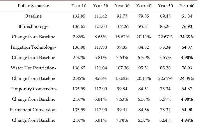
The beginning regional average saturated thickness was 152.3 feet, with Dallam County having a thickness of 128 feet, Hartley 153 feet, Moore 162 feet, and Sherman 192 feet. In the unrestrained baseline scenario, the regional average sa-turated thickness declines 53.4% during the 60-year planning horizon to reach a level of 61.8 (Table 1). In Dallam County, the saturated thickness declined 61.5% reaching 49.2 feet, Hartley 52.1% to 73.2 feet, Moore 65.5% to 55.8 feet, and Sherman 61.2% to 70.6 feet (Table 2).

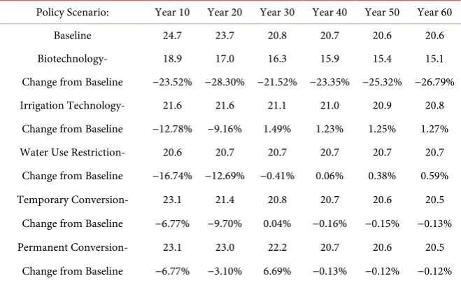
[image:8.595.210.541.513.721.2]

As the water level declines, well capacity drops and irrigation costs rise, lead-ing to less water belead-ing required to reach a profit maximizlead-ing level of water use. As the per acre water use is decreased, producers shift production from water inten-sive crops (corn) to crops that require less water (sorghum) or to dry land crops. In the baseline scenario, the regional average water use per irrigated acre dropped from 25.3 acre-inches to 20.6 acre-inches by year 60 (Table 3), and the regional average irrigated acres as a percent of total crop acres declined from 72.1% to 27.3% (Table 4). In the individual counties, Dallam County drops from 81.4%

Table 1. Regional average saturated thickness (feet).

Policy Scenario: Year 10 Year 20 Year 30 Year 40 Year 50 Year 60 Baseline 132.85 111.42 92.77 79.35 69.45 61.84 Biotechnology- 136.65 121.04 107.26 95.31 85.20 76.93 Change from Baseline 2.86% 8.63% 15.62% 20.11% 22.67% 24.39% Irrigation Technology- 136.00 117.90 99.85 84.52 73.34 64.87

Change from Baseline 2.37% 5.81% 7.63% 6.51% 5.59% 4.90% Water Use Restriction- 136.65 121.04 107.26 95.31 85.20 76.93 Change from Baseline 2.86% 8.63% 15.62% 20.11% 22.67% 24.39% Temporary Conversion- 135.99 117.90 99.84 84.51 73.34 64.87

Change from Baseline 2.37% 5.81% 7.63% 6.51% 5.59% 4.90% Permanent Conversion- 135.99 117.90 99.91 84.56 73.37 64.90

Change from Baseline 2.37% 5.81% 7.70% 6.57% 5.64% 4.94%

(9)

[image:9.595.210.539.89.313.2]

Table 2. Change in saturated thickness (feet) by county.

Policy Scenario: Dallam Hartley Moore Sherman

Year 1 Year 60 Year 1 Year 60 Year 1 Year 60 Year 1 Year 60 Baseline 128.0 49.2 153.0 73.2 162.0 55.8 182.0 70.6 Biotechnology 128.0 61.5 153.0 89.9 162.0 65.7 182.0 92.7

Change from Baseline 24.9% 22.7% 17.6% 31.2%

Irrigation Technology 128.0 52.2 153.0 76.5 162.0 57.6 182.0 74.6

Water Use Restriction 128.0 61.5 153.0 89.9 162.0 65.7 182.0 92.7

Temporary Conversion 128.0 52.2 153.0 76.5 162.0 57.6 182.0 74.6

Permanent Conversion 128.0 52.2 153.0 76.5 162.0 57.7 182.0 74.6

Table 3. Average water use per irrigated acre (acre-inches).

Policy Scenario: Year 10 Year 20 Year 30 Year 40 Year 50 Year 60

Baseline 24.7 23.7 20.8 20.7 20.6 20.6

Biotechnology- 18.9 17.0 16.3 15.9 15.4 15.1 Change from Baseline −23.52% −28.30% −21.52% −23.35% −25.32% −26.79% Irrigation Technology- 21.6 21.6 21.1 21.0 20.9 20.8

Change from Baseline −12.78% −9.16% 1.49% 1.23% 1.25% 1.27% Water Use Restriction- 20.6 20.7 20.7 20.7 20.7 20.7

Change from Baseline −16.74% −12.69% −0.41% 0.06% 0.38% 0.59% Temporary Conversion- 23.1 21.4 20.8 20.7 20.6 20.5

Change from Baseline −6.77% −9.70% 0.04% −0.16% −0.15% −0.13% Permanent Conversion- 23.1 23.0 22.2 20.7 20.6 20.5

Change from Baseline −6.77% −3.10% 6.69% −0.13% −0.12% −0.12%

The average is based on the total water use (at time = t) divided by the total irrigated acres (at time = t) for the region.

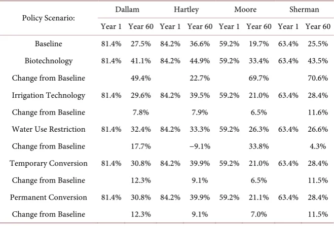
of all crop acres under irrigation to 27.5% of all acres in year 60, Hartley from 84.2% to 36.6%, Moore 59.2% to 19.7%, and Sherman from 63.4% to 25.5% (Table 5).

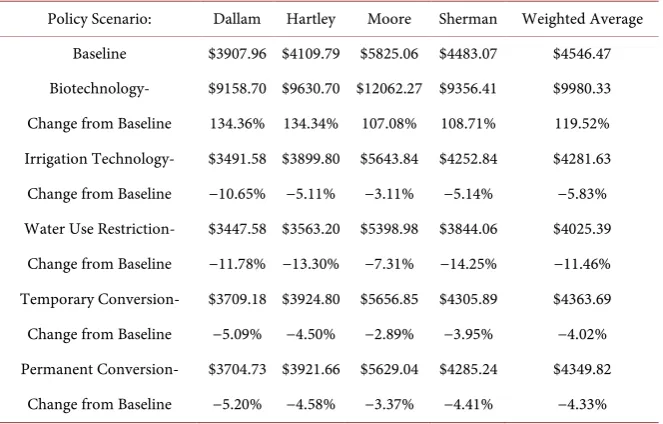
The regional average net income per acre drops 48% from $191.26 to $100.30 per acre as producers shift their production away from irrigated crops (Table 6). These returns yield an average net present value per acre in the baseline scenario of $4564 (Table 7).

[image:9.595.209.539.344.546.2]

(10)

[image:10.595.211.540.90.292.2]

Table 4. Average irrigated acres as a percentage of total crop acres.

Policy Scenario: Year 10 Year 20 Year 30 Year 40 Year 50 Year 60 Baseline 72.10% 72.10% 62.07% 45.15% 34.46% 27.25% Biotechnology- 71.99% 71.20% 65.03% 57.57% 49.65% 40.86% Change from Baseline −0.15% −1.24% 4.77% 27.50% 44.07% 49.93% Irrigation Technology- 69.35% 69.35% 68.04% 50.59% 37.92% 29.59% Change from Baseline −3.82% −3.82% 9.62% 12.04% 10.05% 8.57% Water Use Restriction- 66.07% 58.40% 51.20% 44.00% 36.81% 29.62%

Change from Baseline −8.36% −19.00% −17.52% −2.54% 6.82% 8.67% Temporary Conversion- 64.89% 69.80% 69.08% 51.31% 38.48% 30.02%

Change from Baseline −10.00% −3.19% 11.28% 13.65% 11.65% 10.15% Permanent Conversion- 64.89% 64.89% 64.89% 51.37% 38.51% 30.04% Change from Baseline −10.00% −10.00% 4.53% 13.78% 11.75% 10.24%

The percentage is based on the total irrigated acres (at time = t) divided by total irrigated and non-irrigated cropland acres in the region.

Table 5. Irrigated acres as a percentage of total crop acres by county.

Policy Scenario: Dallam Hartley Moore Sherman

Year 1 Year 60 Year 1 Year 60 Year 1 Year 60 Year 1 Year 60 Baseline 81.4% 27.5% 84.2% 36.6% 59.2% 19.7% 63.4% 25.5% Biotechnology 81.4% 41.1% 84.2% 44.9% 59.2% 33.4% 63.4% 43.5%

Irrigation Technology 81.4% 29.6% 84.2% 39.5% 59.2% 21.0% 63.4% 28.4%

Water Use Restriction 81.4% 32.4% 84.2% 33.3% 59.2% 26.3% 63.4% 26.6%

Change from Baseline 17.7% −9.1% 33.8% 4.3%

Temporary Conversion 81.4% 30.8% 84.2% 39.9% 59.2% 21.0% 63.4% 28.4%

Permanent Conversion 81.4% 30.8% 84.2% 39.9% 59.2% 21.1% 63.4% 28.4%

declines 52.0% to reach a level of 61.5 feet, Hartley declines 41.3% to 89.9 feet, Moore 59.5% to 65.7 feet, and Sherman 49.1% to 92.7 feet (Table 2). In this sce-nario, average water use per irrigated acre drops to 15.1 acre-inches (Table 3), which is 26.8% less than in the baseline scenario.

[image:10.595.209.539.351.574.2]

(11)

[image:11.595.209.540.88.293.2]

Table 6. Average net income per acre.

Policy Scenario: Year 10 Year 20 Year 30 Year 40 Year 50 Year 60 Baseline $183.99 $174.44 $147.16 $123.32 $109.27 $100.30 Biotechnology- $252.02 $336.47 $422.27 $507.26 $588.28 $661.21 Change from Baseline 36.97% 92.88% 186.95% 311.33% 438.36% 559.25% Irrigation Technology- $165.60 $160.19 $151.63 $127.07 $111.00 $101.04

Change from Baseline −10.00% −8.17% 3.04% 3.04% 1.58% 0.74% Water Use Restriction- $159.82 $146.99 $134.46 $123.07 $112.67 $103.11

Change from Baseline −13.14% −15.74% −8.63% −0.21% 3.11% 2.80% Temporary Conversion- $164.66 $165.23 $157.62 $131.42 $114.24 $103.56

Change from Baseline −10.51% −5.28% 7.11% 6.57% 4.54% 3.25% Permanent Conversion- $164.66 $163.21 $156.75 $131.53 $114.30 $103.59

Change from Baseline −10.51% −6.44% 6.52% 6.65% 4.60% 3.29%

The average is based on the total irrigated and non-irrigated net revenue (at time = t) divided by total irri-gated and non-irriirri-gated cropland acres in the region.

Table 7. Average net present value of returns per acre.

Policy Scenario: Dallam Hartley Moore Sherman Weighted Average Baseline $3907.96 $4109.79 $5825.06 $4483.07 $4546.47 Biotechnology- $9158.70 $9630.70 $12062.27 $9356.41 $9980.33 Change from Baseline 134.36% 134.34% 107.08% 108.71% 119.52% Irrigation Technology- $3491.58 $3899.80 $5643.84 $4252.84 $4281.63 Change from Baseline −10.65% −5.11% −3.11% −5.14% −5.83% Water Use Restriction- $3447.58 $3563.20 $5398.98 $3844.06 $4025.39

Change from Baseline −11.78% −13.30% −7.31% −14.25% −11.46% Temporary Conversion- $3709.18 $3924.80 $5656.85 $4305.89 $4363.69 Change from Baseline −5.09% −4.50% −2.89% −3.95% −4.02% Permanent Conversion- $3704.73 $3921.66 $5629.04 $4285.24 $4349.82

Change from Baseline −5.20% −4.58% −3.37% −4.41% −4.33%

Regional average net return (weighted by total cropland acres in each county) per acre discounted over a 60-year planning horizon at a discount rate of 3% per year.

Dallam County, irrigated acreage increases 49.4% over the baseline reaching 41.1% of total acres, Hartley 22.7% to reach 44.9%, Moore 69.7% to reach 33.4%, and Sherman 70.6% to reach 43.5% (Table 5). Average net income per acre in-creases significantly due to the increased yields this scenario provides, reaching $661.21 per acre or 559.3% more than the baseline (Table 6). This equates to a net present value of $9,980 per acre, which is 119.5% higher than in the baseline

(Table 7). It should be noted that the assumptions in this scenario are based on

[image:11.595.209.541.351.563.2]

(12)

In the irrigation technology adoption scenario, the regional average saturated thickness drops 57.5% to 64.9 feet in year 60 of the simulation, which is 4.9% higher than the baseline scenario level (Table 1). In Dallam County, the satu-rated thickness declines 59.2% to reach a level of 52.2 feet, Hartley declines 50.0% to 76.5 feet, Moore 64.4% to 57.6 feet, and Sherman 59.0% to 74.6 feet

(Table 2). In this scenario, average water use per irrigated acre drops to 20.8

acre-inches (Table 3), which is 1.27% higher than in the baseline scenario. Irrigated acres as a percent of all cropland acres in this scenario increases above the baseline in year 60 by 8.57% to 29.59% of all acres (Table 4). Here again, the increase in irrigated acreage in the later years is due to more water being available in those years because of less water usage in earlier years of the simulation. In Dallam County, irrigated acreage increases 7.8% over the baseline reaching 29.6% of total acres, Hartley 7.91% to 39.5%, Moore 6.5% to 21.0%, and Sherman 11.6% to 28.4% (Table 5). Average net income per acre increases 0.74% from the baseline by year 60, reaching $101.04 per acre (Table 6). This equates to a net present value of $4,282 per acre, which is 5.83% less than in the baseline (Table 7).

In the water use restriction scenario, the regional average saturated thickness drops 49.7% to 76.9 feet in year 60 of the simulation, which is 24.4% higher than the baseline scenario level (Table 1). In Dallam County, the saturated thickness declines 52.0% to a level of 61.5 feet, Hartley declines 41.3% to 89.9 feet, Moore 59.5% to 65.7 feet, and Sherman 49.1% to 92.7 feet (Table 2). In this scenario, average water use per irrigated acre drops to 20.7 acre-inches (Table 3), which is 0.59% more than in the baseline scenario.

Irrigated acres as a percent of all cropland acres in this scenario increase above the baseline in year 60 by 8.67% to reach 29.62% of all acres (Table 4). This in-crease in irrigated acreage is also due to more water being available in the later years as a result of less water usage in earlier years of the simulation. In Dallam County, irrigated acreage increases from 17.7% to 32.4% of total acres, Hartley decreases 9.1% to 33.3%, Moore increases 33.8% to 26.3%, and Sherman increases 4.3% to reach 26.6% (Table 5). Average net income per acre increases 2.8% from the baseline by year 60, reaching $103.11 per acre (Table 6). However, the net present value of these returns decreases from the baseline by 11.46% at $4025 per acre due to the increased annual returns occurring later in the scenario (Table 7).

The regional average saturated thickness drops 57.54% to 64.9 feet in year 60 in the temporary conversion to dryland scenario, which is 4.90% higher than the baseline scenario level (Table 1). In Dallam County, the saturated thickness de-clines 59.2% to reach a level of 52.2 feet, Hartley dede-clines 50.0% to 76.5 feet, Moore 64.45% to 57.6 feet, and Sherman 59.0% to 74.6 feet (Table 2). In this scenario, average water use per irrigated acre drops to 20.5 acre-inches (Table 3), which is 0.13% less than in the baseline scenario.

(13)

(Table 4). In Dallam County, irrigated acreage increases from 12.3% to 30.8% of total acres, Hartley increases 9.1% to 39.9%, Moore increases 6.5% to 21.0%, and Sherman increases 11.5% to 28.4% (Table 5). Average net income per acre for the region increases 3.25% from the baseline by year 60, reaching $103.56 per acre (Table 6). However, the net present value of these returns is 4.02% less than the baseline at $4364 per acre due to increased annual returns occurring later in the scenario (Table 7).

The permanent conversion to dry land scenario provided results similar to the temporary conversion to dry land scenario. Under the permanent conversion policy, the regional average saturated thickness drops 57.53% to 64.9 feet in year 60 of the scenario, which is 4.94% higher than the baseline scenario level (Table 1). In Dallam County, the saturated thickness declined 59.2% to a level of 52.2 feet, Hartley declined 50.0% to 76.5 feet, Moore however declined 64.36% to 57.7 feet, and Sherman 59.0% to 74.6 feet (Table 2). In this scenario, average water use per irrigated acre dropped to 20.5 acre-inches (Table 3), which is 0.12% less than in the baseline scenario.

Average irrigated acres as a percent of all cropland acres in this scenario in-creased above the baseline in year 60 by 10.24% to reach 30.04% of all acres

(Table 4). In Dallam County, irrigated acreage increased 12.3% over the baseline

reaching 30.8% of total acres, Hartley increased 9.1% to reach 39.9%, Moore in-creased 7.0% to 21.1%, and Sherman inin-creased 11.5% to 28.4% (Table 5). Aver-age net income per acre for the region increased 3.29% from the baseline by year 60, reaching $103.59 per acre (Table 6). However, the net present value of these returns is 4.33% less than the baseline at $4,350 per acre due to increased annual returns occurring later in the scenario (Table 7).

4. Conclusions

Following are the major conclusions drawn from this research:

 _{The policies that show the most favorable results in terms of conserving the} water available in the Ogallala Aquifer are the biotechnology adoption scena-rio and the water use restriction scenascena-rios. Both policies assume a 1% reduc-tion in water use per year during the 60-year planning horizon.

 _{The permanent conversion to dry land scenario proves to be the third best in} water conservation, though it is just marginally better than the temporary conversion to dry land and the irrigation adoption scenarios.

 The effect of each policy on the saturated thickness in the individual counties varies primarily due to the dependence each county has on irrigated acreage. For example, Sherman County has the greatest water savings in terms of ending saturated thickness in both the biotechnology and water use restric-tion scenarios when compared with the baseline scenario, but it also has the second least irrigated acreage as a percent of total cropland acres.

(14)

irrigated wheat with Dallam having 46.6% in irrigated corn and 28.4% in ir-rigated wheat and Hartley having 49.8% in irir-rigated corn and 25.4% in irri-gated wheat.

 Moore and Sherman counties, however, have a greater reliance on dry land crops. In Moore County, 34.5% of all cropland acreage is in dry land wheat, 23.6% in irrigated corn, and 14.5% in irrigated wheat. In Sherman County, dry land wheat accounts for 32.3% of all cropland acres, while irrigated corn accounts for 25.3% and irrigated wheat 24.3%.

 _{In terms of economic costs, the biotechnology adoption policy by far} vides the greatest net returns and net present values. The yield increases pro-vided in the models are based on seed varieties that are currently available to producers and do not include expected improvements in the future.

 _{The next best policy for the region and each individual county in terms of net} present value of returns is the irrigation adoption technology, though it ranks last (along with the temporary conversion to dry land policy) in terms of re-ducing aquifer depletion. The water use restriction policy, though as effective as the biotechnology adoption policy, has the lowest net present value of re-turns showing that, at present, it would be the best conservation policy but at a significant cost to producers.

5. Limitations and Need for Future Research

As is the case with most studies, there are limitations to the study at hand. These are mainly with regard to the economic model using county average hydrologic data where in reality the hydrological features may vary from one part of the county to another. Further, production functions for each county were estimated using data from the crop simulation software CropMan which is based on only one weather station and the most predominant soil type. Actual county average crop yields are used for dry land crops; however, yields can vary greatly from one area of a county to another. Also, economic parameters and irrigation tech-nology are assumed to be constant during the planning time frame. Finally, com-petition among farmers and between farmers and other residents, for use of avail-able groundwater is not included in the model.

(15)

re-gion and the individual counties while also providing an insight into the impact each policy will have on net farm returns during the 60-year planning horizon.

Acknowledgements

The research is funded, in part, by the Ogallala Aquifer Program, a consortium of the USDA Agricultural Research Service, Kansas State University, Texas AgriLife Research, Texas AgriLife Extension Service, Texas Tech University, and West Texas A & M University. This research is also supported, in part, by the Killgore Research Center and Dryland Agriculture Institute of West Texas A & M Uni-versity.

References

[1] Stewart, B. (2003) Aquifers, Ogallala. In: Stewart, B.A. and Howell, T., Eds., Encyc-lopedia of Water Science, Marcel Dekker, New York, 43-44.

[2] Jensen, R. (2004) Ogallala Aquifer: Using Improved Irrigation Technology and Wa-ter Conservation to Meet Future Needs. Texas WaWa-ter Resource Institute.

[3] Postel, S. (1998) Water for Food Production: Will There Be Enough in 2005. BioSci- ence, 48, 629-637.https://doi.org/10.2307/1313422

[4] Ryder, P.D. (1996) Geological Survey-Ground Water Atlas of the United States, Oklahoma, and Texas. http://capp.water.usgs.gov/gwa/ch_e/E-text5.html

[5] McMahon, P., Dennehy, K., Bruce, B., Böhlke, J., Michel, R., Gurdak, J. and Hurl-but, D. (2006) Storage and Transit Time of Chemicals in Thick Unsaturated Zones under Rangeland and Irrigated Cropland, High Plains, United States. Water Re-sources Research, 42, W03413.https://doi.org/10.1029/2005WR004417

[6] Gurdak, J. and Roe, C. (2009) Recharge Rates and Chemistry Beneath Playas of the High Plains Aquifer—A Literature Review and Synthesis. U.S. Geological Survey Circular 1333, 39 p.

[7] Bilby, T., Bruno, R., Lager, K. and Jordan, E. (2010) Panhandle Water Use: Dairy and Other Commodities. Texas AgriLife Extension Service.

http://texashelp.tamu.edu/004-natural/pdfs/2010-panhandle-water-use-dairy-other-commodities.pdf

[8] Howell, T. (2001) Enhancing Water Use Efficiency in Irrigated Agriculture. Agro- nomy Journal, 93, 281-289.https://doi.org/10.2134/agronj2001.932281x

[9] Pfeiffer, L. and Lin, C. (2010) Does Efficient Irrigation Technology Lead to Reduced Groundwater Extraction? Empirical Evidence. Agricultural and Applied Economics Association Annual Meeting, Denver, 25-27 July 2010, 1-40.

[10] Ward, F. and Pulido-Velazquez, M. (2008) Water Conservation in Irrigation Can Increase Water Use. Proceedings of the National Academy of Science, 105, 18215- 18220.https://doi.org/10.1073/pnas.0805554105

[11] NASS (National Agricultural Statistical Service) (2014) Farm and Ranch Irrigation Survey (2013). 2012 Census of Agriculture. http://www.nass.usda.gov/census [12] Texas Water Development Board (2015) Groundwater Conservation Districts.

http://www.twdb.texas.gov/groundwater/conservation_districts/

[13] Texas Legislature (2015) Texas Senate Bills 1.

http://www.legis.state.tx.us/Home.aspx

(16)

78th Legislature.

[16] Department of Water, Perth, Australia (2009) Policy on Water Conservation/Effi- ciency Plans: Achieving Water Use Efficiency Gains through Water Licensing. Ope- rational Policy No. 1.02.

[17] ARMCANZ (Agriculture and Resource Management Council of Australia and New Zealand) (1996) Allocation and Use of Groundwater: A National Framework for Improved Groundwater Management in Australia. Occasional Paper No 2. Com-monwealth of Australia.

[18] NGC (National Groundwater Committee) (2004) Definition and Approach to Sus-tainable Groundwater Yield. Department of the Environment and Heritage, Canbe- rra.

http://www.environment.gov.au/resource/definition-and-approach-sustainable-gro

undwater-yield

[21] Texas Legislature (2015) Texas Senate Bills 1, 2, 3, 4.

[22] Brooke, A., Kendrick, D., Meerdus, A., Raman, R. and Rosenthal, R.E. (2007) GAMS: A User’s Guide. GAMS Development Corporation, Washington DC. [23] Texas Water Development Board (2001) Survey of Irrigation in Texas, Austin,

Tex-as: TWDB Report 347.

https://www.twdb.texas.gov/conservation/agriculture/irrigation/

[24] Panhandle Water Planning Group (2006) 2006 Regional Plan. Panhandle Regional Planning Commission, Amarillo. http://panhandlewater.org/2006_reg_plan.html [25] Panhandle Water Planning Group (2011) 2011 Adopted Plan. Panhandle Regional

Planning Commission, Amarillo.

http://panhandlewater.org/2011_adopted_plan.html

[26] Feng, Y. and Segarra, E. (1992) Forecasting the Use of Irrigation Systems with Tran- sition Probabilities in Texas. Texas Journal of Agriculture and Natural Resources, 5, 59-66.

[27] Terell, B., Johnson, P. and Segarra, E. (2002) Depletion of the Ogallala Aquifer: Eco- nomic Impacts on the Texas High Plains. Water Policy, 4, 33-46.

https://doi.org/10.1016/S1366-7017(02)00009-0

[28] Wheeler-Cook, E., Sagarra, E., Johnson, P., Johnson, J. and Willis, D. (2008) Water Conservation Policy Evaluation: The Case of the Southern Ogallala Aquifer. Texas Journal of Agriculture and Natural Resources, 21, 87-100.

[29] Das, B., Willis, D. and Johnson, J. (2010) Effectiveness of Two Water Conservation Policies: An Integrated Modeling Approach. Journal of Agricultural and Applied Economics, 42, 695-710.https://doi.org/10.1017/S1074070800003898

[30] Guerrero, B., Amosson, S. and Almas, L. (2008) Integrating Stakeholder Input into Water Policy and Development. Journal of Agricultural and Applied Economics, 40, 465-471.https://doi.org/10.1017/S1074070800023750

(17)

Submit or recommend next manuscript to SCIRP and we will provide best service for you:

Accepting pre-submission inquiries through Email, Facebook, LinkedIn, Twitter, etc. A wide selection of journals (inclusive of 9 subjects, more than 200 journals)

Providing 24-hour high-quality service User-friendly online submission system Fair and swift peer-review system

Efficient typesetting and proofreading procedure

Display of the result of downloads and visits, as well as the number of cited articles Maximum dissemination of your research work