Quasi bayesian estimation of stress strength model for the power function distribution

QUASI BAYESIAN ESTIMATION OF STRESS STRENGTH MODEL FOR THE POWER FUNCTION

1*

1

_{Department of Management Studies, Federal Institute of science and Technology,}

2

_{Department of Mathematics, Union Christian College, Aluva}

ARTICLE INFO ABSTRACT

The reliability of a system is the probability that when operating under stated environmental conditions,

system X and the stress Y as random vari

applied to it exceeds the strength and the component will function satisfactorily whenever X>Y. The quasi-likelihood function was introduced by

unknown parameters in generalized linear models. In Quasi

posterior distribution the likelihood function could be replaced with the natural exponential of the quasi-likelihood function. This method reduces to the usual Bayesi

likelihood and the log estimates for the stress performance of the estimators

Copyright © 2015 Dhanya and Jeevanand. This is an open access article distributed under the Creative Commons Att use, distribution, and reproduction in any medium, provided the original work is properly cited.

INTRODUCTION

The problem of estimating the probability that one random variable exceeds another, that is, interest where X and Y are independent random variables. The parameter

arises in the classical stress–strength reliability where one is interested in assessing the proport

X of a component exceeds the random stress

the system that uses the component may malfunction. This problem also arises in situations w

two devices and has to estimate the probability that one fails before the other. Some practical examples can be found in (1984) and Weerahandi and Johnson (1992).

Hall provided an example of a system application w

of a transverter (power supply) in order for a component to work properly. Weerahandi and motor experiment data where X represents the chamber burst strength and

proposed inferential procedures for P(X > Y)

papers that considered the stress–strength reliability problem, and for references see the recent article by Guo and (2004) or the book by Kotz et al. (2003). The quasi

estimating the unknown parameters in generalized linear models. The idea of quasi

know exactly the distribution of the random component in the model, and replace it by an assumption about how the variance changes with the mean. The quasi-likelihood f

function. Wedderburn (1974) and McCullagh and Nelder (1983) properties similar to the maximum likelihood estimate of t

*Corresponding author: Dhanya, M.,

Department of Management Studies, Federal Institute of science and Technology, Angamaly, Kochi

ISSN: 0975-833X

Vol.

Article History:

Received 16th _{August, 2015}

Received in revised form 22nd _{September, 2015}

Accepted 28th _{October, 2015}

Published online 30th _{November,2015}

Key words:

Reliability,

Stress Strength Model, Power Function Distribution, Quasi Bayesian Estimation

Citation: Dhanya, M. and Jeevanand, E.S., 2015. “

International Journal of Current Research, 7, (11),

REVIEW ARTICLE

QUASI BAYESIAN ESTIMATION OF STRESS STRENGTH MODEL FOR THE POWER FUNCTION

DISTRIBUTION

*

_{Dhanya, M. and}

2

_{Jeevanand, E.S.}

Department of Management Studies, Federal Institute of science and Technology,

Department of Mathematics, Union Christian College, Aluva-2, Kerala

ABSTRACT

The reliability of a system is the probability that when operating under stated environmental conditions, the system will perform its intended function adequately. We consider the strength of the system X and the stress Y as random variables. The component fails at the instant that the stress applied to it exceeds the strength and the component will function satisfactorily whenever X>Y. The

likelihood function was introduced by Wedderburn (1974)

own parameters in generalized linear models. In Quasi-Bayesian Estimation to construct a posterior distribution the likelihood function could be replaced with the natural exponential of the

likelihood function. This method reduces to the usual Bayesi

likelihood and the log-likelihood function are identical. In this paper, we obtain Quasi Bayesian estimates for the stress –strength reliability for the power function distribution. We illustrate the performance of the estimators using a simulation study.

is an open access article distributed under the Creative Commons Attribution License, which use, distribution, and reproduction in any medium, provided the original work is properly cited.

The problem of estimating the probability that one random variable exceeds another, that is, R =

are independent random variables. The parameter R is referred to as the reliability parameter. This problem strength reliability where one is interested in assessing the proportion of the times the random strength of a component exceeds the random stress Y to which the component is subjected. If X ≤ Y, then either the component fails or the system that uses the component may malfunction. This problem also arises in situations where

two devices and has to estimate the probability that one fails before the other. Some practical examples can be found in

Hall provided an example of a system application where the breakdown voltage X of a capacitor must exceed the voltage output of a transverter (power supply) in order for a component to work properly. Weerahandi and Johnson (1992)

represents the chamber burst strength and Y represents the operating pressure. These authors

P(X > Y) assuming that X and Y are independent normal random variables. There are several

ength reliability problem, and for references see the recent article by Guo and The quasi-likelihood function was introduced by Wedderburn (1974)

generalized linear models. The idea of quasi-likelihood weakens the assumption that we know exactly the distribution of the random component in the model, and replace it by an assumption about how the variance likelihood function could be used for estimation in the same way as the usual likelihood McCullagh and Nelder (1983) showed that the maximum

quasi-properties similar to the maximum likelihood estimate of the vector  (the vector of parameters in regression models).

Department of Management Studies, Federal Institute of science and Technology, Angamaly, Kochi-683577. International Journal of Current Research

Vol. 7, Issue, 11, pp.22921-22927, November, 2015

INTERNATIONAL

2015. “Quasi bayesian estimation of stress strength model for the power function distribution 7, (11), 22921-22927.

QUASI BAYESIAN ESTIMATION OF STRESS STRENGTH MODEL FOR THE POWER FUNCTION

Department of Management Studies, Federal Institute of science and Technology, Angamaly, Kochi-683577

2, Kerala

The reliability of a system is the probability that when operating under stated environmental the system will perform its intended function adequately. We consider the strength of the ables. The component fails at the instant that the stress applied to it exceeds the strength and the component will function satisfactorily whenever X>Y. The Wedderburn (1974), to be used for estimating the Bayesian Estimation to construct a posterior distribution the likelihood function could be replaced with the natural exponential of the likelihood function. This method reduces to the usual Bayesian estimation if the

quasi-In this paper, we obtain Quasi Bayesian strength reliability for the power function distribution. We illustrate the

ribution License, which permits unrestricted

= P(X > Y), has been continuous is referred to as the reliability parameter. This problem ion of the times the random strength , then either the component fails or here X and Y represent lifetimes of two devices and has to estimate the probability that one fails before the other. Some practical examples can be found in Hall

of a capacitor must exceed the voltage output Y Johnson (1992) presented a rocket– represents the operating pressure. These authors are independent normal random variables. There are several ength reliability problem, and for references see the recent article by Guo and Krishnamoorthy Wedderburn (1974), to be used for likelihood weakens the assumption that we know exactly the distribution of the random component in the model, and replace it by an assumption about how the variance unction could be used for estimation in the same way as the usual likelihood -likelihood estimates have many (the vector of parameters in regression models).

INTERNATIONAL JOURNAL OF CURRENT RESEARCH

Also, if the underlying distribution comes from a natural exponential family the maximum quasi-likelihood estimate maximizes the likelihood function and so it has full asymptotic efficiency; under more general distributions there is some loss of efficiency, which had been investigated by Hill and Tsai (1988). Youssef (2009) introduce the maximum quasi-likelihood estimates of the unknown parameters of the Pareto distribution and new quasi-Bayesian method of estimation. Many man made and naturally occurring phenomena including city sizes, incomes, word frequencies and earth quake magnitudes are distributed according to a power-law distribution.In the field of information technology the power law distribution is widely used in Networking and web trafficking. For example a power law distribution can be used to model the usage time of the commercial web site by any customer, the time interval having maximum visit etc. In fact a power law implies that small occurrence are extremely common, where as large instance are extremely rare.

Quasi-Bayesian Estimation

In Quasi-Bayesian Estimation to construct a posterior distribution the likelihood function could be replaced with the natural exponential of the quasi-likelihood function. This method reduces to the usual Bayesian estimation if the quasi-likelihood and the log-likelihood function are identical. Let x x₁, ₂,...,x_n be an independent random sample, with mean  ( ), where  is a vector of parameters, and the variance var (x) =

V

( )



, where V(.) is some known variance function, and  is a dispersion parameter which could be known or unknown. The quasi-likelihood Q(x,,) can be derived as defined by the relation

( ,

_{i i}

)

i

Q x









=

(

)

i i

i

x

V







(1.1)

and the natural exponential of Q(x,,) will be used as a likelihood function. Using a suitable prior density

g

( , )

 

the posterior distribution





1

( ,

)

exp{ ( , , )}

( , )

n

i

f

 

x

Q x

 

g

 







 









(1.2)

where





 

( )

,





( ,

 

_{1 2}

,...,



_n

)

and  >0. Consider the power function distribution

1

,

( , , )

x

, 0

,

0

f x

x



 

 

  















_

_











_(1.3)

Mean and variance of X

E(X) =

 

(

1)

1



and V(X) =

  

2

(

1) (

2



2)

1





(1.4)

So if we take  = E(X) =

 

(

1)

1



, we have V(X) =

2











_







V() , with V()= 2



, is the variance function. Thus for a

sample

x x

₁

,

₂

,...,

x

_n of size n, the quasi-likelihood function is given by

2

i

x

n

Q

















which gives

( , )

Q x



=

x

i

n

ln











substituting for  we get

Q

(x,

 

₁

, )

= ( 1) 1 ln( )

n

 



 

 

  (1.5)

with

1

n

i i

x





To obtain the posterior density of (, ) we take natural exponent of Q(x, , ) as the likelihood function. So we have



x

 

,





= ( 1)n ( 1)

n e

 _ 

 

 

 . (1.6)

We consider the prior of α =



p1

e



, , ,

p

 

0



(1.7)

The joint posterior density function f(α,β) is as follows

1( 1) 1 ( 1)

( , ) [ (1)] exp ,

n p

qb n

f   x C     

 

      

   

 

 

α>0,β>0

1

0 0

( 1) ( 1)

( ) exp

n p

qb n

C d d











d d

 





 

   

 

 __  _

 

 

 

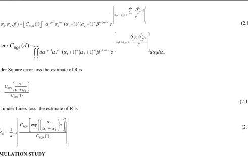
ESTIMATION OF STRESS STRENGTH RELIABILITY

Let X and Y are two independent power function distribution random variables with parameters (1, ) and (2, ) respectively. Therefore

R =P(X>Y)= ( 1 1) ( 2 1)

1 2

0 0

(1

)

(1

)

x

x



y



dydx

 



 





   





 

= 2

1 2









. (2.1)

Now we consider this in two cases

(i) known

In the inference problem considered here we assume that the scale parameter is  known and both1 and2 are greater than 2.

Let x = (x1, …, xn) is random sample from power (1, ). Taking the gamma prior

 

1 1

1 1

, ,

0,

1

0

p

g



_





e

 

p



_



_

(2.2)

The quasi posterior density of 1 is obtained as



1



f



x

=



₁p1

1

(

1)

n





_e

1T_{, 1>0. (2.3)}

where T=( 1 n

i i

x







_



)

Similarly let y = (y1, …, ym) is random sample from power distribution (2, ). Taking the gamma prior

 

1 2

2 2

, ,

0,

2

0

q

g







e

 

q











(2.4)

The posterior density,

f





₂

y



=



₂q1

(



₂



1)

m

_e

2S_{,α2>0 (2.5)}

Where S=( 1

m j j

y  







₎

1 1 2

( ,

) [

_RQB

(1)]

f

 

C







₁p1

(



₁



1)

n



₂q1

2

(





1)

m

_e

(1T2S)_{, 1,2>0 (2.6)}

Where

( )

RQB

C

d

= ₁ 1

2 2

p

d



  

 

(

1

1)

n







₂q1

2

(





1)

m ( 1 2 )

1 2

T Z

e

 

d

 

d

. (2.7)

Under Square error loss the estimate of R is

2

1 2

(1)

SL

RQB

RQB

C

R

C

























(2.8)

and under Linex loss the estimate of R is

2

1 2

1

ln

exp

(1)

LL RQB

RQB

R

C

a

aC











_

_

_

_









_







_





















(2.9)

(ii)β unknown

In this case we suggest the joint prior distribution for the parameters as

g(1, ) = g1(1) g2(1) (2.10)

where g1(1) 1-1 (2.11)

which is the Jeffrey’s non-informative prior and a gamma prior for



1 as

 

1

1

2 1 1 1

( )

, , ,

0

(

1)

p p

g

e

p

p

 







 













(2.12)

Hence using (2.11) and (2.12) the joint posterior density is obtained as









( 1) 1

1

,

1

1

1

exp

1

n

i

n p n i

x

f

 

x









T



  



































,where 1

n

i i

x

T







 



(2.13)

Similarly let y = (y1, …, ym) is random sample from power function distribution (2, ). Then the posterior density of 2 based

on a gamma prior









( 1) 1

2, 2 1 2 exp 2

m j

m q m j

y

f   y     Z



  

 

 

 

   

 

 

 



(2.14)

where 1

m

j j

y

Z

















1 1 1 2

( )

1 _{1 1 ( )}

1, 2, (1) 1 2 ( 1 1) ( 2 1)

n m i j i j

x y

T Z

p q n m m n

RQB

f C e

                             _{   }      

_{ }   (2.15)

Where

C

_RQB

( )

d

=

1 1

1 2

( )

1 1 ( )

1 2 1 2 1 2

2 2

( 1) ( 1)

n m

i j

i j

x y

T Z

p q n m m n

d e d d

  











 

                            

 

Under Square error loss the estimate of R is

2 1 2 (1) SL RQB RQB C R C        _     (2.16) and under Linex loss the estimate of R is

2 1 2 exp 1 ln (1) LL RQB RQB C a R a C            _  _        _{ }       (2.17) SIMULATION STUDY

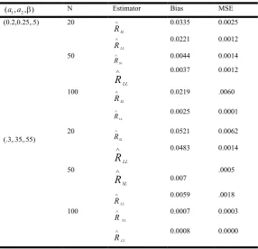
In order to assess the performance of the estimators, we perform a simulation study of 2000 samples of sizes n = 10, 20, 50 and 100 generated from power function distribution for values of (1,2) = (0.2,0.25),(0.3,0.35),( 0.4,0.45) and (0.5,0.55). The estimators was evaluated for the prior hyper-parameters p, = 1 and 2. We present the simulation results concerning the bias and mean square errors of all these estimators. In all the simulation results presented here, the bias of an estimator can be determined as the average value of the estimate report in the table – True value. The variance of an estimator was determined as the sample variance obtained from all the simulations carried out. Finally, the mean square error of estimator is (variance of the estimator + (Bias)2). The bias and mean squared errors (in parentheses) of the estimators are presented in Tables .

[image:5.595.47.539.44.357.2]

Tables

Table 1.β Known, when τ=1 and p=1

(1,2) N Estimator Bias MSE

(0.2,0.25) 20

SL

R

 0.0424 0.0125

LL R

 _{0.0342 0.006}

50

SL

R

 0.0354 0.0157

LL R

 _{0.0122 0.0014}

100

SL R

 _{0.007 0.0002}

LL

R

 _{0.002 0.0003}

(0.3,0.35) 20

SL R

 _{0.0533 0.0125}

LL R

 _{0.0483 0.0014}

50

SL

R

 0.0067 .0005

LL R

 _{0.0049 .0002}

100

SL

R

 0.007 .0003

LL

R

[image:6.595.155.442.74.350.2]

Table 2. β Unknown, when τ=1 and p=1

1, 2, )

(a a  N Estimator Bias MSE

(0.2,0.25,.5) 20

SL R

 0.0335 0.0025

LL R

 0.0221 0.0012

50

SL R

 _{0.0044 0.0014}

LL

R

 0.0037 0.0012

100

SL R

 0.0219 .0060

LL R

 _{0.0025 0.0001}

(.3,.35,.55)

20

SL

R 0.0521 0.0062

LL

R

 0.0483 0.0014

50

SL

R



0.007

.0005

LL R

 _{0.0059 .0018}

100

S L R

 _{0.0007 0.0003}

LL R

 0.0008 0.0000

Conclusion

We obtained the estimators of the reliability function. From the table we can observe that the estimate under Linex Loss function has lesser bias and MSE than the squared error loss. Also the bias and the MSE reduces as the sample size increases.

REFERENCES

Abu-Salih, M.S. and Shamseldin, A.A. 1988. Bayesian estimation of P(X<Y) for a bivariate exponential distribution, Arb Gulf J.Sci. Res. A, Math.Phys. Sci., 6(1), 17-26.

Awad, A.M, Azzam, A.M. and Hamdan, M.A. 1981. Some inference results on Pr(X<Y) in the bivariate exponential model, Communications in Statistics - Theory and Methods, 10(24), 2515-2525.

Bai, D.S. and Hong, Y.W. 1982. Estimation of Pr(X<Y) in the exponential case with common location parameters, Communications in Statistics, Theory and Methods, 21, 269-282.

Beg, M.A. 1980c. On the estimation of P(Y<X) for the two parameter exponential distribution, Metrika, 27, 29-34.

Beg, M.A. 1980a. Estimation of P(Y<X) for truncated parameter distribution, Communications in Statistics, Theory and Methods, 9, 327-345.

Constantine, K., Karson, M. and Tse, S.K. 1986. Estimation of P(Y<X) in the gamma case, Communications in Statistics, Computation and Simulation, 15, 365-388.

Cramer, E. 2001. Inference for stress-strength models based on Wienman multivariate exponential samples, Communications in Statistics, Theory and Methods, 30, 331-346.

Guo, H. and Krishnamoorthy, K. 2004. New approximate inferential methods for the reliability parameter in a stress-strength model: The normal case. Communication in Statistics – Theory and Methods, 33, 1715–1731.

Hall, I.J. 1984. Approximate one-sided tolerance limits for the difference or sum of two independent normal variates. J Qual Technol 16:15–19

Hangal, D .1995 Testing reliability in a bivariate exponential stress-strength model, Journal of Indian Statistical Association, 33, 41-45.

Hill, J. R. and Tsai, C.L. 1988. Calculating the efficiency of maximum quasi-likelihood estimation. Apple. Statist. 37, 2, 219 – 230.

Kotz, S., Lumelskii, Y and Pensky, M 2003. The Stress-Strength Model and its Generalizations. World Scientific, London.

Kundu, D. and Gupta, R.D. 2005. “Estimation of P(Y < X) for Generalized Exponential Distribution,” Metrika, vol. 61(3), pp. 291-308.

McCullagh, P. and Nelder, J.A. 1983. Generalized linear models. London: Chapman and Hall.

Weerahandi, S, and Johnson, R.A. 1992. "Testing Reliability in a Stress -Strength Model when X and Y are Normally distributed,"Technometrics, 34, 83-91

Youssuf .M. S 2009. Bayesian estimation for the Pareto parameters using Quasi Likelihood function ,Applied mathematical sciences ,vol.3,2009,no.11,509 -517.