DOI: 10.4236/apm.2019.92006 Feb. 20, 2019 78 Advances in Pure Mathematics
Rongchuan Tao
1, Yingzi Yang
2, Xiaoxiao Zou
3, Zifan Dong
4, Siran Chen
51School of Management, Wuhan University, Wuhan, China 2City University of Hong Kong, Hong Kong, China 3Pilgrim School, Los Angeles, USA
4Weiyu High School, Shanghai, China 5The SMIC Private School, Shanghai, China
Abstract
This research paper concentrates on the Kakeya problem. After the introduc-tion of historical issue, we provide a thorough presentaintroduc-tion of the results of Kakeya problem with some examples of the early solutions as well as the proof of the final outcome of this problem, the solution of which is known as Besicovitch Set. We give 3 different construction of Besicovitch set as well as the intuition of construction, which is related to iterated integral of 2-variable real function. We also give the Cunningham construction in which the area of a simply connected Kakeya set can also tend to 0. Furthermore, we generalize the process of generating a Kakeya set into a Kakeya dynamic. The definition of multiplicity enables us to estimate the area of a Kakeya set. In following discussion we provided a conjecture related to the solution in particular range. Finally, the derivation of the Kakeya problem is presented.
Keywords
Kakeya Needle Problem, Besicovitch Set
1. Introduction
1.1. History of Kakeya Problem
In 1917, Sōichi Kakeya asked a question: what is the smallest area which enables a unit line segment to rotate 180 degrees and return to the initial position in re-versed direction? In honor of Kakeya, a compact set E⊂n in which the unit line segments can be found in every direction is defined to be Kakeya set.
1, n, . . , 1 12 2, . n
S x s t x t E t
ξ − ξ
∀ ∈ ∃ ∈ + ∈ ∀ ∈ −
How to cite this paper: Tao, R.C., Yang, Y.Z., Zou, X.X., Dong, Z.F. and Chen, S.R. (2019) The Kakeya Problem. Advances in Pure Mathematics, 9, 78-110.
https://doi.org/10.4236/apm.2019.92006
Received: November 13, 2018 Accepted: February 17, 2019 Published: February 20, 2019
Copyright © 2019 by author(s) and Scientific Research Publishing Inc. This work is licensed under the Creative Commons Attribution International License (CC BY 4.0).
http://creativecommons.org/licenses/by/4.0/
DOI: 10.4236/apm.2019.92006 79 Advances in Pure Mathematics where Sn−1 is the notation for unit sphere in n. The optimal solution for the Kakeya problem when n = 2 is constructed by Besicovich, known as Besicovich set.
1.2. History of Besicovitch
Abram Samotlvitch Besicovich made great contributions to the Kakeya problem. Described in [1], his family had seven children and they were living in a frugal life. The older ones earned money to support the younger ones. They all studied at the University of St. Petersburg and received high education. After his gradu-ation, Besicovitch published his first paper about probability theory. Later in 1917, he became a professor in the University, which was destroyed in 1919 during the Civil War. However, Besicovitch locked books in the cellar and pre-served most of the property, which later contributed to the re-establishment of the university after the liberation of Perm. In 1920, he returned to Leningrand and gave lectures on Pedagogical Institute for four years. However, from 1920, as the Russian revolution was launched, he was forced to lecture to workers who had weak mathematical backgrounds. To leave Russia, he decided to apply for Rockefeller Fellowship, a fellowship that enabled people to work abroad, but the offer was not obtained until 1924.
Accompanied with another mathematician, J.D. Tamarkin, Abram Besico-vitch went to Copenhagen. In Copenhagen, he worked with Harald Bohr for a year. Then, he made his way for Oxford and stayed for several months with G.H. Hardy, who recognized his great analytical talent and enabled his lectureship at the University of Liverpool for 1926-1927. In 1927, he moved to Cambridge and became a college lecturer as well as a Fellow of Trinity.
Besicovitch passed most of his life in Britain. After retiring from the Rouse Ball Chair in 1958, he remained active in the field of mathematics as a visiting professor in the United States. After all, he died in his eightieth year on 2 No-vember, 1970. Besicovitch is a successful mathematician who received several high standard awards and medals and his mathematical work is still valuable to-day and still influences the modern mathematical field.
1.3. The Structure of This Paper
DOI: 10.4236/apm.2019.92006 80 Advances in Pure Mathematics keya problem. In Section 6, we provide the recent result and algebraic analog of the Kakeya problem under finite field context. One of the most famous results is the size of finite field Kakeya conjecture which has been proved in Divr [4]. Also, some other derivatives discussed in Pugh [5] and Furtner [6] are also included. The summary of this paper is in Section 7.
2. Some Examples of Kakeya Sets
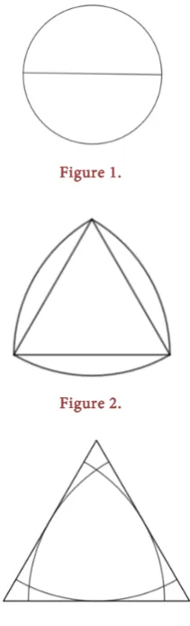
2.1. Circle
Details. Rotate a unit needle centered at its midpoint for 180˚, forming a circle (see Figure 1).
Area calculation. Let the length of the needle be 1. The area of the circle is 2
1 π π 0.785
2 4
i
S = = =
.
2.2. Curved Edge Triangle
Details. Combine three identical 60˚ sectors together to form a convex triangle. The edges of the sectors form an equilateral triangle. The needle starts from an edge of the triangle, then rotates 60˚ for three times in order to reverse itself (see
Figure 2).
Area calculation. Let the length of the needle be 1, so the length of the side of each sector 1. The area of each sector is π
6
i
S = , where i = 1, 2, 3. The area of
inner triangle is 3
4
S′ = . The total area of the convex triangle is
π 3 π
2 0.705
6 4 6
S= − + =
.
2.3. Equilateral Triangle
Details. Combine three identical 60˚ sectors together to form an equilateral tri-angle. The needle starts from one side of the triangle with one end of needle at a vertex of the triangle, rotates to another side of the triangle, then slides a little to the another vertex of the triangle. Repeat the process three times. Then, the needle reverses itself (see Figure 3).
Area calculation. Assume the length of the needle be 1, so the height of the equilateral triangle equals to 1. The area of the triangle is 1 0.577
3
DOI: 10.4236/apm.2019.92006 81 Advances in Pure Mathematics
Figure 1.
Figure 2.
Figure 3.
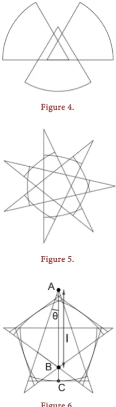
2.4. Sunshape
Details. Since both the equilateral triangle and the convex triangle are both composed of three identical sectors with 60˚ (see Figure 4), which can construct a semicircle without overlapping. Then, we can cut the semicircle into smaller sectors and construct them to a smaller figure. For example, the figure composed of seven sectors is similar to the seven-point star except the seven small sectors between the outer triangles (see Figure 5).
Area calculation. Since the figure was composed of the a n-point star and n
sectors, divide the area into two parts for calculation. Let the angle of half of the outer triangles be θ, then 2π
2n 1
θ=
+ . Then make an angle bisector from one of the vertex A to intersect the n-point star with point B, and intersect the arc of the sector with point C. Let the length of AB be l (see Figure 6). Since the calcu-lation of small sector is complicated, make a line tangent to the arc of the sector at point C to form a small triangle. Let the length of the needle be 1, then
1
AC= , BC= −1 l. The area S of the whole figure is
( )
( )
( )
( )
(
)
( )
2 2
2 2
2
sin sin
1 1 tan 3
sin 2 sin 2
S n l θ θ n l θ
θ θ
= ⋅ ⋅ ⋅ − + ⋅ − ⋅
DOI: 10.4236/apm.2019.92006 82 Advances in Pure Mathematics
Figure 4.
Figure 5.
Figure 6.
Then the area of figure with five sectors is
( )
(
(
)
(
)
(
)
)
2
2 3 3 5 5 20 5 1 10 5 1
4 5 5
l l
S l = + − + + +
−
Then the minimum area of the figure with five sectors is 0.542 when l = 0.921. When the semicircle is cut into n pieces, it can achieve its minimum area. When n goes to ∞, θ goes to 0. The area of the shape is
(
)
2 23 π 3π 1
16 2
S= l + −l
The minimum area of this figure is 0.524 when 8
9
l= .
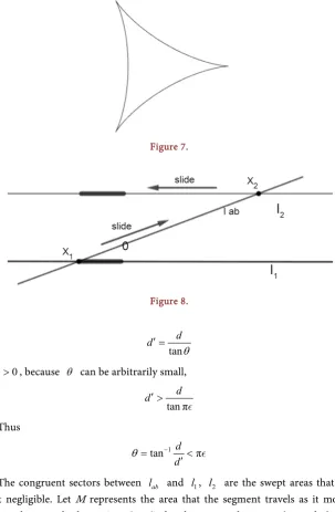
2.5. Deltoid
[image:5.595.313.433.72.492.2]DOI: 10.4236/apm.2019.92006 83 Advances in Pure Mathematics Kakeya problem. One can intuitively understand the formation of a deltoid in
[7]. It’s also easy to see how it is qualified for a Kakeya set: the needle starts from the middle of the deltoid which one of the ends is at a vertex of the deltoid and another end is at the middle point of the side. The needle rotates along and keeps tangent to the side. The same process repeats three times. The needle re-verses itself (see Figure 7).
Area calculation. Build an x-axis and a y-axis. The function of deltoid curve can be presented on the coordinate which is
( ) (
)
cos cos(
R r t)
x t R r t r
r
−
= − +
( ) (
)
sin sin(
R r t)
y t R r t r
r
−
= − −
where R represents the radius of the large circle which is 3
2, and r represents
the radius of the rolling circle which is 1
2. Take the data into the function and
then we can calculate the area S:
( )
(
)
3π
2 2 2
2 3π 2 3π 2 3 3 3π 2 1
d sin 2 2sin cos 4sin cos 2sin cos 8
1 1 1sin 4 2sin 4cos 1cos 2 π
8 2 8 3 3 2 8
S y x t t t t t t t
t t t t t
− − = = + − − = − + + + =
∫
∫
3. Besicovitch Set
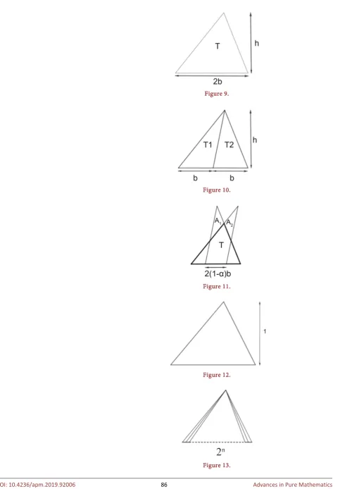
3.1. Translation between Parallel Line
To deal with the Kakeya problem, the trick named Pàl joins is established to achieve the minimum rotating area.
Given two parallel lines l1, l2, Let x1 be any point in l1, and x2 be a point in l2. Connect the two points and name the line across x1, x2 as lab. Let the angle between lab and l1 (or l2) be θ. Assume that the original po-sition of the unit segment is in l1. Move that unit segment such that one of its endpoint reaches x1. Then rotate the segment to coincide with lab, and slide to
2
x . Finally, rotate the unit segment to l2. Since the area cost depends on θ, when the theta becomes extremely small, the unit line segment can “jump” from
1
l to l2 cost a very small area (see Figure 8). The following lemma is the proof of this strategy.
1 Lemma. Let l1, l2 be parallel lines. ∀ > 0, ∃ a compact set E s.t.
E <, in which any unit line segment can be moved continuously from l1 to 2
l .
DOI: 10.4236/apm.2019.92006 84 Advances in Pure Mathematics
Figure 7.
Figure 8.
tan
d d
θ ′ =
0
∀ > , because θ can be arbitrarily small,
tanπ
d d′ >
Thus
1
tan d π
d
θ = − <
′
The congruent sectors between lab and l1, l2 are the swept areas that are not negligible. Let M represents the area that the segment travels as it moves along the straight lines. Let S1, S2 be the sectors between lab and l1, l2 with unit radius. Take E M S= 1 S2. M can be arbitrary small and S1, S2<2,
so E<.
3.2. Besicovitch Sets
The lemma above implies the possibility to construct a compact set which is Le-besgue measure zero and contains unit line segments in every direction. There are two methods to construct the Besicovitch set which satisfies the conditions.
Method 1. First, we show the original version Besicovitch set which has been simplified to be the Perrontree.
DOI: 10.4236/apm.2019.92006 85 Advances in Pure Mathematics length b (see Figure 10). Slide T1, T2 along the bottom line at a contrary di-rection such that the overlapped length of their bottom is 2 1
(
−α)
b, where1 1
2≤ ≤α . Let the area of T be T . The area S of this new figure, containing
two small triangles A1, A2 above and a triangle T1, which is similar to T, at the base (see Figure 11) is
(
)
(
2 2 1 2)
S = α + −α T
Proof. The bottom side length of T1 is 2αb. So 2
1
T =
α
TThe line, parallel to the bottom side and across the vertex of T1, divides A1, A2 into four triangles A11, A12, A21, A22 (see Figure10). A11 is congruent to
22
A , and A12 is congruent to A21. The bottom length of them is
(
1−α)
b and the height is(
1−α)
h. Thus the area of A1 and A2 is(
)
1 2 1
A = A = −α T
Thus the total area of T1 is
(
)
(
2 2)
1 2 1 2 1
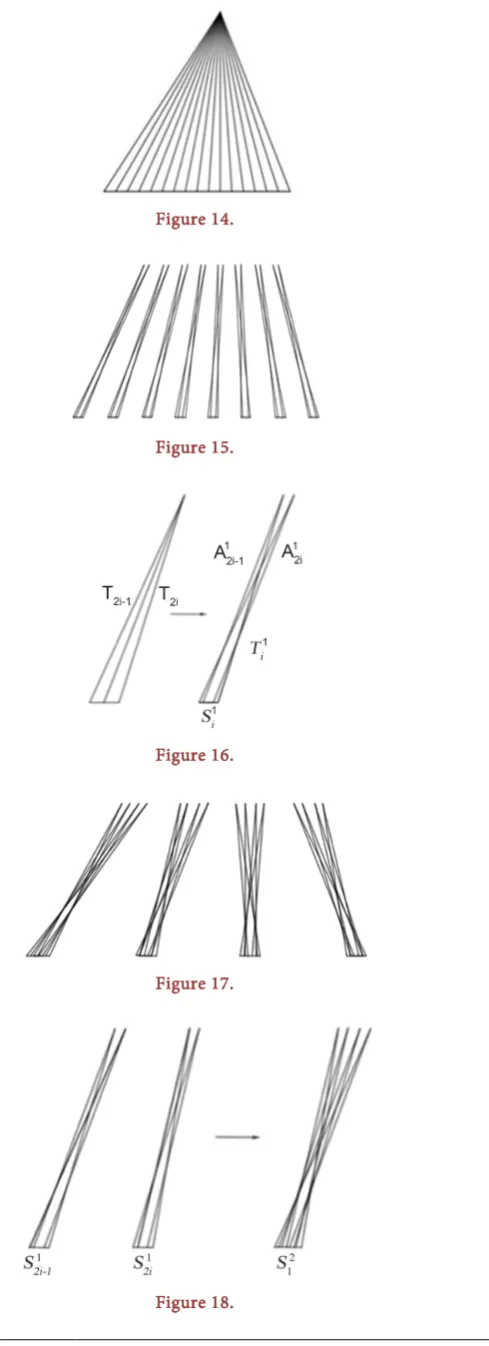
S= A + A +T = α + −α T Based on this construction technique and the lemma above, we can construct the Perron tree as follows:
Given a triangle with height 1 (see Figure 12), divide the bottom of 2n equal pieces and get 2n triangles (see Figure 13).
Step 1, move the adjacent triangles T2 1i− , T2i (1≤ ≤i 2n−1) with the same technique and get 2n−1 figures called 1
i
S (see Figure 14 & Figure 15). The top two small triangles are called 1
2 1i
A − , A12i and basal triangle is called Ti1 (see
Figure 16). One side of T2 1i− is parallel and equal to the other side of T2i, so
1
i
S is translated such that 1
i
T forms a triangle called T1 which is similar to T. Step 2, move the adjacent figures 1
2 1i
S − , S12i (1≤ ≤i 2n−2) to form Si2 and name the basal triangle as 2
i
T (see Figure 17 & Figure 18). Translate 1
i
S to let
1
i
T form a triangle which is similar to T called T2.
Step r (2≤ ≤r n), move the adjacent figures
S
2 1ri−−1,S
2ri−1 (1≤ ≤i 2n r− ) toform r i
S . and name the basal triangle as r i
T . Translate r i
S to let r i
T form a triangle named Tr which is similar to T (see Figure 19).
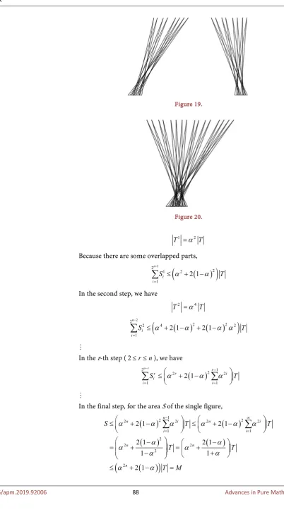
In the final step, we can obtain a single figure with 2n small triangles above and one basal triangle Tn. This is the Perrontree (see Figure 20).
3 Theorem. The measure of the Perrontree can be arbitrary small.
Proof. In the first step, from lemma() we have
(
)
(
2)
1 2 2 1 1
i i
S = α + −α T
From the translation of 1
i
DOI: 10.4236/apm.2019.92006 86 Advances in Pure Mathematics
Figure 9.
Figure 10.
Figure 11.
Figure 12.
[image:9.595.282.531.67.740.2]DOI: 10.4236/apm.2019.92006 87 Advances in Pure Mathematics
[image:10.595.56.547.67.755.2]Figure 14.
Figure 15.
Figure 16.
Figure 17.
DOI: 10.4236/apm.2019.92006 88 Advances in Pure Mathematics
Figure 19.
Figure 20.
1 2
T =α T
Because there are some overlapped parts,
(
)
(
)
1 2 2 1 2 1 2 1 n ii S α α T
−
=
≤ + −
∑
In the second step, we have
2 4
T =α T
(
)
(
)
(
)
2
2 2 2
2 4 2
1 2 1 2 1
n
i
i S T
α α α α
−
=
≤ + − + −
∑
In the r-th step (2≤ ≤r n), we have
(
)
2 2 1
2 2
1 1
2 1
n r r
r r i
i
i S i T
α α α
− − = = ≤ + −
∑
∑
In the final step, for the area S of the single figure,
(
)
(
)
(
)
(
)
(
)
(
)
1 2 22 2 2 2
1 1
2
2 2
2 2
2 1 2 1
2 1 2 1
1 1
2 1
n
n i n i
i i
n n
n
S T T
T T
T M
α α α α α α
DOI: 10.4236/apm.2019.92006 89 Advances in Pure Mathematics when α→1 and nT→ ∞, ∀ > 0, M <. Thus S can be arbitrary small.
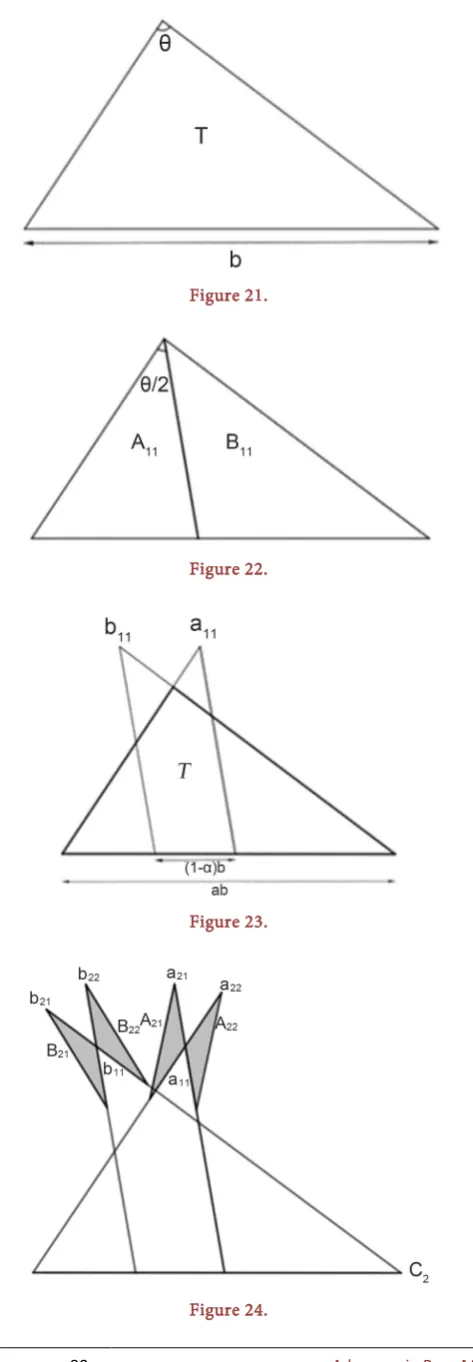
Method 2. The other attempt of constructing such set is simpler in a tricky way.
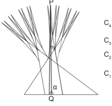
Given a triangle T with vertex θ and bottom length b (see Figure 21), cut the triangle from its angle bisector into two pieces marked as A11, B11 (see
Figure 22).
Move the two pieces along the bottom line at the opposite direction such that the overlapped length at the bottom is
(
1−α)
b, where 0≤ ≤α 1. Let the newfigure be set C1. The basal triangle similar to T is named as T′. Thus the bot-tom length of T′ is αb. Let the vertex of triangle A11 be a11, and the vertex of triangle B11 be b11. The angles of those two vertex are both 2
θ
(see Figure 23).
Extend the sides of A11 to points a21, a22 such that the distances between 21
a , a22 and a11 are 1. Let two lines pass the point a21 and a22 and be pa-rallel to the angle bisector of A11 then we can obtain two small triangles named
21
A , A22. Repeat the steps above for B11 and get other two triangles B21, B22. We call the small triangle “horn”. The apex angles of those four triangles are
4
θ . Set C2 =
{
A A B B21, 22, 21, 22}
(see Figure 24).Extend the side of A21, A22, B21, B22 and get eight smaller “horns”, named A31, A32, A33, A34, B31, B32, B33, B34. The set contains them called
3
C (see Figure 25).
Continually repeat the manipulations above, we can get a set E like a “tree”.
n
∀ ∈, Cn contains 2n “horns”, whose apex corners are
2n θ
.
4 Lemma. ∀ ∈n , n≠1, ∀A A B Bni, nj, nr, ns∈Cn, where i j r s, , , ∈ 1,2n−1 and i j≠ , r s≠ , Ani ≅ Anj ≅Bnr ≅Bns.
Proof. For each triangle in Cn, because its bottom is parallel to the angle bi-sector of the corresponding triangle in Cn−1, it must be an isosceles triangle with basal angle
2n θ
and the lengths of the isosceles sides are 1 (see Figure 26).
Also, because the third angle of them are π 1
2n θ
−
− , every triangle in Cn satisfies the condition of the congruent theorem “ASA”. Thus, every triangle in Cn is congruent.
5 Lemma. ∀ ∈n , n≠1, assume the area of Cn is cn, then cn<2θ.
Proof. For each “horn” in Cn, the area of it is less than the area sum of two sectors with radius 1 and angle
2n θ
. Therefore, 2 2 2 2
n
n n
c < θ = θ
. Assume that the area of the whole overlapped graph of A11, B11 is c1, which is a constant. So, for the total area of the “tree”,
(
)
1 1 1
2 22 2 1
n n
n
i i
c c c c θ c n θ
= =
DOI: 10.4236/apm.2019.92006 90 Advances in Pure Mathematics
Figure 21.
Figure 22.
Figure 23.
DOI: 10.4236/apm.2019.92006 91 Advances in Pure Mathematics
Figure 25.
Figure 26.
Let h=min
{
d a x(
ni, ni)
,d b y(
nj, nj)
}
(1 ,≤i j≤2n−1), whereni
a , bni are the vertexes of the triangles in Cn satisfies that the segment which connected itself and its projection point is in the “tree”, and xni, ynj are the projection points. For the chosen vertex P, the extension cord of its adjacent side which is length 1 insects with the bottom at Q such that d P Q
(
,) (
= n− +1)
a, where a>0. Let the anglebetween the extension cord and the bottom be
α
. Thus, h=(
n− +1)
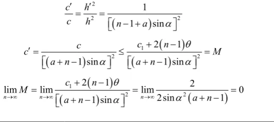
asinα (see Figure 27).Compress the whole “tree” proportionally to obtain a new set E′ which is similar to the previous set E and h becomes h′, where h′ =1. Let the basal tri-angle be T′′. After the compression, for the whole area c′,
(
)
2 2 2 1 1 sin c hc h n a α
′ ′ = = − +
(
)
(
)
(
)
1 2 2 2 11 sin 1 sin
c n c
c M
a n a n
θ α α + − ′ = ≤ = + − + −
(
)
(
)
(
)
1 2 22 1 2
lim lim lim 0
2sin 1
1 sin
n n n
[image:14.595.249.523.616.738.2]DOI: 10.4236/apm.2019.92006 92 Advances in Pure Mathematics
Figure 27.
Therefore, E′ achieves the arbitrary small area.
6 Lemma. E′ contains a unit line segment in every direction in θ.
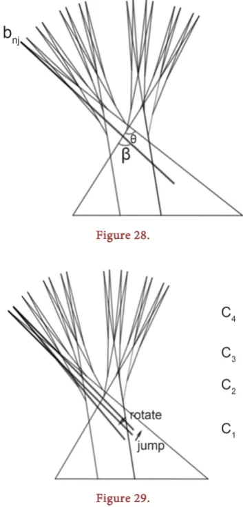
Proof. Assume that after compressing, Cn becomes Cn′. Because E′ is similar to E, Cn′ is similar to C. For set E′, ∀ set Cn′, the sum of the apex is θ. Fix one endpoint of the unit line segment at ani or bnj, where 1 ,≤i j≤2n−1. Assume the angle between the unit segment and the left side of T′′ be β (see
Figure 28).
First, we prove that every β∈
[ ]
0,θ can be found in E′. Note that every adjacent triangle in Cn has a parallel and equal side. Let Ibj = {β: β can be taken when unit segment rotates inside Bnj} and Iai = {β: β can be taken when unit segment rotates inside Ani}. Then we have(
)
(
)
1
1 1
, , , , 0,
2 2 2 2
bj n n b n bn n
j n
j
I =θ− θ θ− − θ I =θ− θ θ I = θ− − θ
(
)
(
)
1
1 1
, , , , 0,
2 2 2 2 2 2 2 2
ai n n a n an n
i n
i
I =θ− θ θ− − θ I =θ θ− θ I = θ− − θ
Therefore,
[ ]
0,θ ⊂(
Iai)
( )
IbjThen, we prove that E′ contain a unit segment every direction in θ. Because h is the minimum distance from the apex to the bottom, the unit segment can reach the bottom only when the endpoint is P′ (corresponding to
P). Thus the unit segment can be contained in every direction in θ in set E′. This lemma indicates that we can rotate the unit segment for every value in θ with the method of Pàljoins. The following is the specific manipulation.
Without the loss of generality, let the unit segment star at the left side. First use the parallel lemma to “jump” to the 2-nd triangle, rotate
2n θ
[image:15.595.217.513.450.558.2]DOI: 10.4236/apm.2019.92006 93 Advances in Pure Mathematics
Figure 28.
Figure 29.
The difference between Kakeya set and Besicovitch set is that Kakeya set per-mits movement. The detailed definition of movement will be discussed in Sec-tion 5.
Method 3. Instead of cutting triangle to form a Besicovitch sets, cutting sector will reduce the waste of cutting triangle (see Figure 30).
Inscribe a sector with the radius the same as the height of the isosceles trian-gle. Since when rotating the needle in the Besicovitch sets, the needle actually only uses the area of sectors without using the whole area of the triangle. So, there are wastes of the areas in using the triangle Besicovitch sets.
Assume a big triangle with the height of 1 is cut into 2n pieces, and T is the set of all small triangles. Then, inscribe a sector with the radius the same as the height of the triangle. Then, cut the sectors into 2n pieces, such that each small piece of the sector is contained in each small triangle. Assume S is the set of all small sectors. So, S T⊂ .
Construct a triangle Besicovitch set, and then take out all the area of T S\ to form a sectorial Besicovitch set. Since the areas of the triangle Besicovitch set equals to and S T⊂ , the area of the sectorial Besicovitch set less than
DOI: 10.4236/apm.2019.92006 94 Advances in Pure Mathematics
Figure 30.
Figure 31.
Figure 32.
Figure 33.
3.3. The Origin of Besicovitch Set
DOI: 10.4236/apm.2019.92006 95 Advances in Pure Mathematics plane 2, the existence of
∫∫
f x y x y( )
, d d does not always imply the existence of∫ ∫
f x y x y(
, d d)
. For example, let f x y(
,)
=1 if x∈, y=0 , and(
,)
0f x y = otherwise. This function is zero except on a single line. Therefore, the discontinuity points comprise a planar zero set, and thus it is Riemann in-tegrable on the plane. However, it is not Riemann inin-tegrable on the slice.
For the case above, a simple manipulation of rotating the coordinate would transform the function into a Riemann integrable function that could be inte-grated by iterated integrals. Besicovitch wondered if there exists a Riemann in-tegrable function f defined on the plane which is free from the choice of ortho-gonal coordinate axes, such that the iterated integral
∫ ∫
f x y x y(
, d d)
cannot substitute the Riemann integral∫∫
f x y x y( )
, d d for all possible linear coordi-nate systems.He found a counterexample by constructing a compact zero set that contains a unit line segment in every direction, known as the Besicovitch set. The characte-ristic function χB is Riemann integrable since the set of discontinuity points is a zero set in plane.
For example, let B = Besicovitch set and let A=
(
×) (
×)
, f =χA B . We can translate B in the y-direction so that some horizontal segments σ ∈0 B have rational y-coordinates y0. Thus χ × =1 on σ0 and f x y(
, 0)
=χ( )
x , which is not Riemann integrable as a function of x. Since A B B ⊂ , we haveA B is a zero set, therefore f is Riemann integrable on the plane. Now, let
(
ξ η,)
be a new set of orthogonal coordinates on the plane.1˚. The ξ-axis is parallel to the x-axis. The segment σ0 is contained in B and parallel to the ξ-axis, but
∫
f x y(
, 0)
dx does not exist (see Figure 34).2˚. The ξ-axis is not parallel to the x-axis. The property of the Besicovitch set implies that B contains a segment: σ =
{
(
ξ η η η, :)
= 0&ξ ≤1}
that is parallel to the ξ-axis. Notice that Aσ is dense inσ
. The discontinuity points of the single variable function f(
ξ η, 0)
would be the whole segmentσ
, which is not a zero set. Thus, f(
ξ η, 0)
is not Riemann integrable (see Figure 35).4. Simply Connected
We construct a simple connected Kakeya set with the 4 following steps. It is contained in a circle of radius 1, and its area can be arbitrarily close to 0 (<).
Step 1. We start with a simple construction. Let Γ be a fixed unit circle and Π be a regular polygon concentric with Γ, having sides of a large odd num-ber Q. The area of Π can be arbitrarily small as long as the radius of its cir-cumcircle is small enough (see Figure 36).
Lem. Take a vertex of Π, denoted as C. Connect the longest diagonals from
DOI: 10.4236/apm.2019.92006 96 Advances in Pure Mathematics
Figure 34.
Figure 35.
Figure 36.
Now consider the area of Π and those triangles. The area of Π, according to the previous discussion, can be arbitrarily close to 0. The sum of those trian-gles, however, will be arbitrarily close to π 2 as long as Q is large enough. (The sum of area of triangles is close to 1 1 1 π 2
2 π
Q Q
⋅ ⋅ ⋅ ⋅ = ).
DOI: 10.4236/apm.2019.92006 97 Advances in Pure Mathematics
Figure 37.
Tree. Tree is improved from J, lies on the right side of x=0. We put the ( )0
K into plane, between two lines x=0 and x=1. The common vertex of ∆ and J is on the line x=δ. We have δ+ =r 1. Denote ∆ as triangle
CA B′ ′, where vertex A′ and A′ are on the line {x=0. Extend A C′ and
B C′ , they intersect the line x=1 at points A and B respectively.
Choose distinct points on segment A B′ ′ in descending order: 0 , , ,1 m 1
C =A C′ C + =B′.
Choose distinct points on segment AB in ascending order: 0 , , , ,1 2 m
V =A V V V =B.
The tree is the union of m+1 triangles: ∆C V Ci i i+1, i=0,1, , m.
Joins. Joins lie on the left side of x=0. For every Ci, extend V Ci−1 i and i i
V C , intersecting the line
x
= −
r
at Ai and Bi respectively. Then we get a triangle Ji = ∆C A Bi i i. Joins are the union of m triangles J1, , Jm.Denote K( )1 =Tree Joins . Now we consider the area of K( )1 . Denote J
S =a (S means area), SJi =ai, then
2 1
1 1 1
2 2 2
i i i i i
a = A B r⋅ = ⋅ ⋅r V V r− ⋅ = ⋅r AB ra=
∑
.In conclusion, the area of Joins is less than the area of J after this improvement (see Figure 38).
Step 3. In this part, we make further improvement of the tree, and prove that the area of tree can be arbitrarily close to zero.
First, we put a triangle ∆ABC between the line x=0 and x h= ′, one side of which (denoted as AB) is on the line x=0. AB =σ. Extend AC and BC, intersecting the line x h= ′′ at V0 and V1 respectively (h′′>h′). The mid-point of AB is M. Connect V M0 and V M1 , intersecting AC and BC at D1 and D0 respectively. Shadow the triangle ∆D CV1 1 and ∆D CV0 0, and the shadow area is the new additional area. We now calculate the shadow area (see
Figure 39).
(
)
2(
)
21 2 2
Shadow
h h h h
S
h h σ h σ
′′− ′ ′′− ′
= ⋅ ⋅ <
DOI: 10.4236/apm.2019.92006 98 Advances in Pure Mathematics
Figure 38.
Figure 39.
Now divide the space between x=δ and x=1 into p equal parts. Take
r i p
δ + ⋅ and r i
(
1)
p
δ + ⋅ + as h′ and h′′, employ the improvement above for p times (Let i=0,1, , p−1). The total area of shadow area is no more than
(
)
2(
)
2 21 1
0 0
p p
i i
r p r p r
i r p p
σ
σ σ
δ δ δ
− −
= =
⋅ < ⋅ =
+ ⋅
∑
∑
. Therefore, SShadow→0 as p→ ∞ (see Figure 40).Step 4. Consider every triangle ∆A B Ci i i in the Joins of K( )1 . Denote
i i i
A B C i
S∆ =a Extend ACi i and B Ci i, intersecting the line x=δ at Ai′ and i
B′ respectively. Let ∆C A Bi i i′ ′ be ∆ in K( )0 ,
i i i
A B C
∆ be J in K( )0 . Then we make improvement following the Step 2 and Step 3, constructing a small “Tree and Joins”. The total area of new joins is no more less than rai. Therefore, if we denote the graph after this improvement as K( )2 ,
Joins
S of K( )2 is less than 2
r a. Take improvements following the above steps, we can get K( )N with N
Joins
DOI: 10.4236/apm.2019.92006 99 Advances in Pure Mathematics
Figure 40.
5. Methodology
The most essential intuition of the Besicovitch set is to cut a basic figure (e.g. a 1
6
disc) into different pieces and overlap the pieces by conducting parallel tech-nique. In general, we can properly break a Kakeya set into 2 pieces such that a unit line segment can move in each subset. Translating one subset such that it is overlapped on another, generating a new set. After conducting Pal-join trick, it’s obvious that a unit line segment can also turn around in the new set, while the overlapping area indicates that the new Kakeya set has a smaller area. Not all Kakeya sets can reduce area by the process. One example is the deltoid curve.
How to define the extent to which a Kakeya set is overlapped? Given a Kakeya set, can we turn it into a set that has no overlapped area? Is there any law that dominates the area of Kakeya set? In order to analyze the question above, proba-bly we need to reconsider the Kakeya set problem in a new way.
Most of our discussions are under the assumption that the slope angle of the segment monotonically increases from 0 to π as the segment turns around in the Kakeya set. The benefit is obvious, since a given slope angle corresponds to a unique position of the segment. The constraint of monotone condition is so strong that it immediately rules out the existence of Pal-joins, which is an essen-tial part of the Besicovitch set shown previously. In an example constructed by Cunningham, a monotone (but not strictly) and simply connected Kakeya set has been proved to exist, since a segment can slide along its direction for any length without costing area. This example will also be ruled out since we require strictly increasing. One natural question is: Is there any possibility that there still exists a Kakeya set with arbitrary small area?
DOI: 10.4236/apm.2019.92006 100 Advances in Pure Mathematics A Kakeya dynamic is a mapping from the interval to real plane:
[ ]
2: 0,π
φ →
( ) ( ) ( )
(
, ,)
t→ x t y t θ t
Subject to the conditions
1) x t
( )
, x t( )
and x t( )
are C1.2) x
( )
0 =y( )
0 =0 and x( )
π =1,y( )
π =0.The meaning of the above definition is: the left endpoint of a unit line seg-ment begins at the origin at the beginning. The position of the endpoint is
( ) ( )
(
x t y t,)
given the moving time t. The points swept by the segment can be expressed as:(
x t u( )
+ cos( ) ( )
θ ,y t u+ sin( )
θ)
,u∈[ ]
0,1 . Since a Kakeya dy-namic is not necessarily monotone, θ( )
t may not be one-one. If it is monotone, it can be simplified to take the following expression.5.2. Definition: Monotone Kakeya Dynamic
A monotone Kakeya dynamic is a mapping from the interval to the real plane:
[ ]
2: 0,π
φ →
( ) ( )
(
x ,y)
θ→ θ θ
Subject to the conditions 1) x
( )
θ and y( )
θ are C1.2) x
( )
0 =y( )
0 =0 and x( )
π =1,y( )
π =0.The meaning turns to be: the left endpoint of a unit line segment begins at the origin with zero slope angle. The position of the endpoint is
(
x( ) ( )
θ ,y θ)
giv-en the slope angle θ. Each point in the Kakeya set takes the form:( )
( ) ( )
( )
(
x θ +tcos θ ,y θ +tsin θ)
.Since the motion is monotone, each slope angle corresponds to unique segment. Thus the above dynamic is well defined.
Since a Kakeya set permits a needle turning around inside it, every Kakeya set corresponds to a dynamic though the dynamic may not be unique.
The above definition enables us study the extent to which a Kakeya set is overlapped. We will soon define the multiplicity to account for it systematically.
5.3. Definition: Dynamic Track
( )
( ) ( )
( )
(
)
[ ]
{
x θ tcos θ ,y θ tsin θ θ θ, : 0,π}
3DOI: 10.4236/apm.2019.92006 101 Advances in Pure Mathematics The track of the dynamic lifts the motion process into 3 space. Through defining a projection mapping, we can deal with the multiplicity of a point in Kakeya set.
5.4.
Definition:ProjectionMapping
A projection mapping is the inverse of the dynamic which sends each point in dynamic track back to the Kakeya set.
: K
Π Ω →
( ) ( )
(
x θ ,y θ θ,)
→(
x( ) ( )
θ ,y θ)
The existence of overlapping guarantees that the projection mapping is an onto but not one-one map. To some extent, it resembles an identification map from Ω to K. Now we can precisely measure the extent to which a Kakeya set is overlapped by examining the cardinality of the pre-image of each point in the Kakeya set.
5.5. Definition: Multiplicity
The multiplicity is a mapping from a Kakeya set to the natural numbers:
:K
λ →
( )
( )
1#
x→ Π− x =
λ
xThe multiplicity of a point is defined to be the cardinality of the pre-image of it with respect to the projection mapping. A highly overlapped Kakeya set auto-matically manifests relatively high multiplicity for each point in it. The area of the set would also become relatively smaller. To precisely express the above thoughts, we define a set that corresponds to a given Kakeya set. The set is named as “unfolded set”, the multiplicity of any point in which is one.
5.6. Definition: Unfolded Set
The unfolded set of a Kakeya dynamic is the set expressed in polar coordinates:
( )
(
)
[ ]
[ ]
{
, : 0,1 , 0,π}
2U = M θ +uθ u∈ θ∈ ⊂
where
( )
cos( )
( )
sin
x M
y
θ θ
θ
θ θ
=
Decompose the motion of the segment into the sliding along direction of the segment and the rotation at the center of a point which lies on the segment or on its extension. Then M
( )
θ is exactly the component of the revolution. The un-folded set is aimed to wipe out the sliding motion of the segment and keep the rotation only. We present the example of the deltoid to illustrate the fact pre-cisely (see Figure 41 & Figure 42).DOI: 10.4236/apm.2019.92006 102 Advances in Pure Mathematics
Figure 41.
Figure 42.
:
F U→K
( )
(
M θ +u,θ)
→(
x( )
θ +usin( ) ( )
θ ,y θ +ucos( )
θ)
The left side is polar coordinates while the right side takes the form of ortho-gonal coordinates. F is a C1 map from U to K.
It would be an immediate result that for any x K∈ , #F−1
( )
x =λ
( )
x . In order to prove our main theorem, we need some lemmas.1 Lemma. Given a partition of a Kakeya set K:
{
i: i ,1}
P= S S ⊂K ≤ ≤i n
Suppose each Si is simply connected area and the map between K and the unfolded set U induced by projection map is F. Then
( )
{
1 : ,1}
i i
P′ = F− S S ∈P ≤ ≤i n
is a partition of U.
Proof. To see P′ is a partition, we need to show that P′ is a cover of U and elements in P′ are disjoint, which is equivalent to: for each p U∈ , there ex-ists unique Si such that p F∈ −1
( )
Si . For each q U∈ , since P is a partition ofK, there exists S P∈ such that F q
( )
∈S, it’s obvious that q is contained in( )
1i
F− s . Thus P′ is a covering of U. Now suppose there exist 1
( )
1F− S and
( )
12
F− S that cover a point p U∈ . We immediately have
( )
1 2
F p ∈S S
DOI: 10.4236/apm.2019.92006 103 Advances in Pure Mathematics 2 Lemma. There is a closed simply connected set
{ }
A ⊂2. Suppose f is a ho-meomorphism from A to B, then B A− ⊂{
x f x,( )
:x∈ ∂A}
, where x f x,( )
means the line segment generated by endpoint: x and f x
( )
.Proof. If B A− is empty, there is no point in B A− . So we only consider the case where B A− is nonempty.
If p∈ ∂B. Since the homeomorphism from A to B induces a
homeomor-phism from ∂A to ∂B, there exists unique preimage of p, denoted by p′, and
p′∈ ∂A. It’s obvious that p∈ p f p′,
( )
′ .Now we suppose that p int B∈
( )
. A is simply connected, f is homeomor-phism, so B is simply connected and ∂B is a Jordan curve. Moreover, notice that p A∉ , so we have: p is encompassed by ∂B while it’s not done by ∂A(see Figure 43). This drastic difference is the point of the proof.
Suppose the perimeter of ∂A is l. Fix a point O∈ ∂A. A point Q is moving
along ∂A, which is a closed curve, from the beginning position O until it back to that original point. Denote the travelled distance of Q to be x, then the slope angle of line PQ would be a continuous function of x, denoting γ
( )
x .The image f Q
( )
=:Q′ is also going a full round along ∂B as Q travels around along ∂A since f is a homeomorphism. The slope angle of PQ′ is also a continuous function of x, denoting θ
( )
x . Without loss of generality, we definethat γ
( )
0 =0, which can be done by rotating x axis. Then, according to theabove fact, we have: γ
( )
l =2π, and θ( )
0 =θ( )
l .To see how the above definition contributes to the proof, notice that there eixsts x0 such that p∈ x f x0,
( )
0 if and only if there exists x0 such that( )
x0( ) (
x0 2k 1)
π,kγ +θ = + ∈ (see Figure 43).
Since there exists k0∈ such that
(
2k0+1)
π−θ( )
0 ∈[
0, 2π]
, weimmediate-ly have: γ
( )
0 +θ( ) (
0 − 2k0+1)
π≤0 and γ( )
l +θ( ) (
l − 2k0+1)
π≤0. Theex-istence theorem of zero point of continuous function claims that there exists
[ ]
0 0,
x ∈ l such that γ
( )
x0 +θ( ) (
x0 = 2k0+1)
π (see Figure 44). 3 Lemma. There is a closed simply connected set{ }
A ⊂2. Suppose f is a homeomorphism from A to B ( B⊂2 ). Then B⊂A D , where( )
( )
: f x x
D =M − x , x is boundary point of A.
Proof. Suppose not, then there exist a point p B∈ such that p A D∉ , which also means that p B A∈ − . According to lemma2, there exists x0∈ ∂A
such that p∈ x f x0,
( )
0 . Hence it’s obvious that p M∈ f x( )0−x0( )
x0 . 4 Lemma. There is a family of closed simply connected measurable set
{ }
2n
A ⊂ with Hausdorff dimension 2, the boundary of An has Hausdorff dimension 1. The diameter dn of An tends to 0 as
n
→ ∞
. Suppose fn is a sequence of homeomorphisms from An to Bn (Bn⊂2) such that ∀ ∈xn An,( )
0
n n
n
f x x
d
−
→ as
n
→ ∞
. Then n n 0n
A B
A
−
→ as
n
→ ∞
.Proof. For each n, Since fn is onto map, Hn:= {Oxn :Oxn is f x
( )
n −xn-neighborhood of xn, ∀ ∈xn An} covers Bn. Denote:
: n
n x
DOI: 10.4236/apm.2019.92006 104 Advances in Pure Mathematics
Figure 43.
Figure 44.
According to Lemma 3, Bn⊂AnDn , we have Bn ≤ An + Dn , i.e.
n n n
DOI: 10.4236/apm.2019.92006 105 Advances in Pure Mathematics On the other hand, fn being a homeomorphism implies that fn is inverti-ble, hence Gn:= {Oxn :Oxn is
( )
1
n n
x − f− x -neighborhood of
n
x , ∀ ∈xn Bn} covers An.
Similarly, we can denote:
: n
n x
D′ =O if xn is boundary point of Bn.
And we have An − Bn ≤ Dn′ . In one word, −Dn ≤ An − Bn ≤ Dn′ . In order to show n n 0
n
A B
A
−
→ as
n
→ ∞
, it suffices to show that n 0n
D A →
as
n
→ ∞
and n 0n
D A
′
→ as
n
→ ∞
.Notice that Dn is a cover of the boundary of An with open discs. The Hausdorff dimension of boundary being 1 implies that n
n
D
d tends to a finite
number as
n
→ ∞
. Similarly, we have n nD d
′
tends to a finite number as
n
→ ∞
.Also, Notice that the Hausdorff dimension of An being 2 implies that 2 n n
A d
tends to a finite number as
n
→ ∞
. In conclusion, nn n
D
A d tends to a finite number as
n
→ ∞
andn
n n
D A d
′
tends to a finite number as
n
→ ∞
, so we have n n 0n
A B
A
−
→ as
n
→ ∞
. Under the C1 setting of the Kakeya dynamic, the following lemma shows that the multiplicity of a Kakeya dynamic is a.e. bounded. This finite condition is useful.5 Lemma. The multiplicity λ
( )
p is almost everywhere bounded in the Ka-keya set K.Proof. Suppose not, then there exists an open neighborhood O K⊂ such that ∀ ∈x O, the multiplicity of x, denoting λ
( )
x , is infinity. O is open impliesthat ∃ a closed segment x y, ⊂O. For each point Z on x y, , there are in-finite many θ ∈i
[ ]
0,π such that their corresponding unit segments go throughZ. By extending the unit segment and x y, to be real line and taking the in-tersection, we naturally induce a mapping h from
[ ]
0,π to if we give a pa-rameterization to the line determined by x y, . Since the intersection of 2 lines in plane exists unless they are parallel, the monotone condition implies that the mapping h is C1 continuous except for a point. Denote by[ ]
a b, the interval corresponding to x y, under the parameterization. Then h should satisfy: for each s∈[ ]
a b, , f−1( )
s is a infinite set in the interval[ ]
0,π , according to Bolza-no-Weierstrass theorem, there exists a convergent subsequence
{
u si( )
}
→u s0( )
as a subset of f−1( )
s . The continuity of f implies that(
( )
)
(
( )
)
0 i
f u s → f u s .
DOI: 10.4236/apm.2019.92006 106 Advances in Pure Mathematics
i
s
, f s′( )
i =0, f is constant and si =s0, a contradiction. Lemma 5 claims that for almost every point p K∈ with multiplicity λ( )
p ,there exist finite segments l l1 2, , , lλ( )p containing p. Without loss of generali-ty, we assume the slope angle of li is θi and θi>θj if i j> . We can ex-press coordinate of the point p in λ
( )
p ways, i.e.( )
( ) ( )
( )
(
i icos i , i isin i)
p= x θ +u θ y θ +u θ .
Suppose F is the mapping from the unfolded set to the Kakeya set constructed previously. F−1
( )
p takes the form of{
(
( )
,)
:1( )
}
i i i
M θ +u θ ≤ ≤i λ p , which is
a collection of λ
( )
p distinct points in U. Take a partition of a Kakeya set K:{
i: i , is simply connected,1i}
P= S S ⊂K S ≤ ≤i n
Given that the diameter of Sk is small enough, F−1
( )
p induce λ( )
p num-ber of homeomorphism fk between sk and a neighborhood of(
M( )
θi +ui,θi)
:i
V , with F V
( )
i =Si.Now we consider a particular homeomorphism, say fk:
:
k k i
f S →V
( )
( ) ( )
( )
(
x θi +ucos θi ,y θi +usin θi)
→(
M( )
θi +u,θi)
The below figure (Figure 45) shows the pattern of the motion in ∆θ neigh-borhood, where the velocity vector
(
x( ) ( )
θ ,y θ)
is decomposed into the nor-mal component and radial component.Computation shows that M
( )
θ is the distance between the rotation center and the endpoint. Take a point q in Sk. Triangle inequality implies that( )
( )
2cot
k
[image:29.595.88.538.587.743.2]f q −q ≤ α θ∆ , while the diameter of Sk ≥u
( )
∆θ . The mesh of Sk is at least: L∆θ, where L is the distance between q and the rotation center. ThusDOI: 10.4236/apm.2019.92006 107 Advances in Pure Mathematics
( )
0
k n
f q q d
−
→ as n→0, so we can apply the lemma1, lemma2, lemma3 and
lemma4 to get theorem 6.
6 Theorem. The integral of multiplicity on Kakeya set K is equal to the area of unfolded set U:
(
, d d)
1d dKλ x y x y= U x y
∫∫
∫∫
Proof. Given a series of partition of Kakeya set K: Pn =
{
S Si: i ⊂K,1≤ ≤i n}
with mesh tends to 0 asn
→ ∞
.The Riemann sum of
∫∫
Kλ( )
x y x y, d d is∑
iλ(
x y si, i)
i . The Riemann sum of∫∫
U1d dx y is 1( )
i i F S
−
∑
. The difference between them is:( , )
( )
1i i
x y
i k i
i k S f S
λ
= −
∑ ∑
.From the lemma above, i k
( )
i 0i
S f S S
−
→ as n→0. Moreover, λ
(
x yi, i)
is almost everywhere bounded on K, we have
(
i, i)
(
i k( )
i)
0i
x y S f S
S
λ −
→ as
n
→ ∞
. So we have( , )
( )
1 0
i i
x y
i k i
i k i i
S f S
S λ
= − →
∑ ∑
∑
asn
→ ∞
.Notice that K is Riemann integrable since x
( ) ( )
θ ,y θ are continuously dif-ferentiable functions. The sum∑
iSi is finite. So( , )
( )
1 0
i i
x y
i k i
i k i i
S f S
S λ
= − →
∑ ∑
∑
as
n
→ ∞
immediately implies: ( , )( )
1 0
i i
x y
i k i
i k S f S
λ
= − →
∑ ∑
asn
→ ∞
.Thus we identify the Riemann sum above. The unfolded set can be regarded as the area swept by a moving unit segment, while the segment must intersect with a fixed point during the whole motion process. It’s obvious that under such constraint, the minimum area of the unfolded set is 1π
2 , obtained by the disc with diameter of 1. We have the following
theo-rem.
7 Theorem. Given a monotone Kakeya dynamic, the integral of multiplicity on Kakeya set is greater than 1π
2 .
( )
, d d 1π 2Kλ x y x y≥
∫∫
It’s a direct deduction that if the area of a sequence of Kakeya sets tends to zero, the multiplicity of points in Kakeya sets must tend to infinity.
Ac-DOI: 10.4236/apm.2019.92006 108 Advances in Pure Mathematics area of strictly monotone Kakeya dynamic.
6. Derivation of Kakeya Problem
Similarly, we can ask the minimum measure that allows a disc or something more general to turn around in some more general spaces (e.g. n-sphere, real projective plane or so). Currently, it has been proved that there exists Kakeya set of arbitrary small measure in sphere. The spherical Kakeya problem reads: In-stead of a plane, the rotation takes place on the surface of a unit sphere and an arc of great circle substitutes the needle. Cunningham showed that for the arc length a: 0≤ ≤a π, the lower bound of Kakeya set area is still 0.
In the range of dimension theory, it was shown by Davies that, in Euclidean spaces, even though Kakeya sets had zero area, they were still necessarily two-dimensional, which led to an analogous conjecture in higher dimensions: the Hausdorff dimension of a Kakeya set is n dimensional Euclidean space. That is the Kakeya conjecture.
1 Conjecture. A Besicovitch set in n has Minkowski and Hausdorff di-mension n.
In an algebraic field, there is an analogous conjecture. The Kakeya set in a fi-nite field Fn is a finite point set K such that for any v F∈ n, there exists a point x F∈ n such that the whole line:
{
x tv t F+ : ∈}
is contained in K. the Kakeya conjecture in Euclidean space takes the form of the finite field conjec-ture.2 Conjecture. Suppose F is finite field and E F⊂ n is a Kakeya set. Then E has cardinality at least n
n
c F , where cn >0 depends only on n.
The finite field Kakeya conjecture was proved by Zeev Dvir in 2008. The me-thod is to combine the Kakeya set with a polynomial which vanishes on that Ka-keya set. The feature of KaKa-keya set implies that any polynomial of degree at most
1
F − which vanishes on a Kakeya set E must be the null polynomial. Then, the cardinality of a Kakeya set must exceed the dimension of the vector space: {P F x∈
[
1, , xn]
: the degree of P is less than F }, which is1 F n n
C + −
.
7. Summary
DOI: 10.4236/apm.2019.92006 109 Advances in Pure Mathematics non-convex sets, mathematicians believed that deltoid was the optimal solution but it was left unproved until Besicovitch found a Kakeya set of arbitrary small area.
We presented 3 methods in constructing Besicovitch sets. The second con-struction is simpler in the sense of estimating the area of each “horn”. The last one makes some minor changes: the unfolded set changes from a triangle to a sector. After the construction, we presented the original intuition of Besicovitch sets, which is connected to the existence of iterated integrals in the real plane.
In 1971, Cunningham provided a simply connected Kakeya set of area less than any real number, which broke through the belief that every simply con-nected Kakeya set had area greater than the Bloom-Schoenberg number. We presented the process of constructing a Cunningham Kakeya set but omitted the proof of simply connectedness.
The Methodology part generalized the trick took place in the Besicovitch set. First, through paraphrasing the Kakeya problem from a dynamic point of view, we defined the multiplicity of a Kakeya set. Then we provided a theorem to ex-plain the fact that if a Kakeya set can achieve arbitrary small area, the set must be highly overlapped. In modern analysis, the concept of multiplicity (not exactly the same though) is also used in estimating the bound of Hausdorff dimension when mathematicians discuss Kakeya maximal functions. The end of this section put forward a conjecture of the constraint under which a deltoid becomes the optimal solution of the Kakeya problem.
There are many forms of the Kakeya needle problem. Many of them were put forward in a relatively modern way. The most important unsolved problem may be the Kakeya conjecture. The algebraic analogue is known as finite-field Kakeya conjecture. The Kakeya conjecture is connected with Fourier analysis, additive combinatorics and partial differential equation.
Conflicts of Interest
The authors declare no conflicts of interest regarding the publication of this pa-per.
References
[1] Taylor, S.J. (1975) Abram Samoilovitch Besicovitch. Bulletin of the London Ma-thematical Society, 7, 191-210. https://doi.org/10.1112/blms/7.2.191
[2] Besicovitch, A.S. (1963) The Kakeya Problem. The American Mathematical Monthly, 70, 697-706. https://doi.org/10.1080/00029890.1963.11992093
[3] Cunningham Jr., F. (1971) The Kakeya Problem for Simply Connected and for Star-Shaped Sets. The American Mathematical Monthly, 78, 114-129.
https://doi.org/10.1080/00029890.1971.11992708
[4] Dvir, Z. (2009) On the Size of Kakeya Sets in Finite Fields. Journal of the American Mathematical Society, 22, 1093-1097.
https://doi.org/10.1090/S0894-0347-08-00607-3