warwick.ac.uk/lib-publications
A Thesis Submitted for the Degree of PhD at the University of Warwick
Permanent WRAP URL:
http://wrap.warwick.ac.uk/93377
Copyright and reuse:
This thesis is made available online and is protected by original copyright. Please scroll down to view the document itself.
Please refer to the repository record for this item for information to help you to cite it. Our policy information is available from the repository home page.
Three Essays in Econometrics
by
Andrea Anita Naghi
Thesis
Submitted to the University of Warwick
for the degree of
Doctor of Philosophy
Department of Economics
Contents
List of Tables iv
List of Figures vii
Acknowledgments ix
Declarations x
Abstract xi
Chapter 1 A Forecast Rationality Test that Allows for Loss
Function Asymmetries 1
1.1 Introduction . . . 1
1.2 Testing Forecast Rationality under Asymmetric Loss: the EKT Framework. . . 5
1.3 Forecast Rationality Tests under Unknown Functional Form of the Loss . . . 8
1.4 Monte Carlo Evidence . . . 12
1.4.1 The Effect of a Misspecified Loss Function in Forecast Evaluation . . . 13
1.5 Empirical Illustration . . . 18
1.6 Conclusion . . . 21
Chapter 2 Global Identification Failure in DSGE Models and its Impact on Forecasting 23 2.1 Introduction . . . 23
2.1.1 Related Literature . . . 27
2.2 The Identification Problem in DSGE Models . . . 32
2.2.1 Setup . . . 32
2.2.2 Definitions . . . 33
2.2.3 Non-identifiability of the ABCD matrices . . . 35
2.2.4 Implications of Identification Failure in Frequentist and Bayesian Analysis . . . 38
2.3 Global Identification Failure: an Illustration . . . 40
2.3.1 The Model of An and Schorfheide (2007) . . . 40
2.3.2 Searching for Observationally Equivalent Parameter Points 44 2.3.3 Numerical Evidence: Linear Model . . . 47
2.3.4 Numerical Evidence: Nonlinear Model . . . 50
2.4 Forecasting with Observationally Equivalent Parameter Points 51 2.4.1 Correct Specification . . . 52
2.4.2 Misspecification . . . 56
2.4.3 Observational Equivalent Structures. . . 63
2.5 Conclusion . . . 66
Chapter 3 Identification Robust Predictive Ability Testing 68 3.1 Introduction . . . 68
3.2.1 Class of Models and Identification Categories . . . 74
3.2.2 Examples . . . 77
3.2.3 Predictive Evaluation Framework . . . 80
3.3 Numerical Evidence: Implications of Identification Loss . . . . 82
3.3.1 Effect on Estimators . . . 82
3.3.2 Effect on Out-of-Sample Tests . . . 85
3.4 Asymptotic Results under Semi-Strong
Identification . . . 88
3.5 Robust Inference . . . 95
3.5.1 Data Dependent Critical Values . . . 96
3.5.2 Simulation: Coverage Probabilities based on Robust Crit-ical Values . . . 98
3.6 Conclusion . . . 101 Appendix A Appendix to Chapter One 102
Appendix B Appendix to Chapter Two 115
List of Tables
2.1 Grid Search Parameter Bounds . . . 46
2.2 Observationally Equivalent Points - Correct Specification . . . 54
2.3 One Step Ahead Point Forecasts - Correct Specification . . . . 55
2.3 CONTINUED: One Step Ahead Point Forecasts - Correct Spec-ification . . . 56
2.4 Observationally Equivalent Points - Misspecification, Output Growth . . . 58
2.5 Observationally Equivalent Points - Misspecification, Inflation 59
2.6 One Step Ahead Point Forecasts - Misspecification, Output Growth . . . 60
2.6 CONTINUED: One Step Ahead Point Forecasts - Misspecifica-tion, Output Growth . . . 61
2.7 One Step Ahead Point Forecasts - Misspecification, Inflation . 62
2.7 CONTINUED: One Step Ahead Point Forecasts - Misspecifica-tion, Inflation . . . 63
2.8 Observationally Equivalent Points - Different Structures. . . . 65
A.2 Rejection frequencies for theJ-test when the forecast evaluation
is done under the true loss function . . . 103
A.3 GMM estimates forα obtained under a misspecified loss function103 A.4 Rejection frequencies for theJ-test when the forecast evaluation is done under a misspecified loss function . . . 104
A.5 Empirical Size and Power for the two tests . . . 105
A.6 J-test based on Median Forecasts . . . 106
A.7 MT-test based on Median Forecasts . . . 107
A.8 J-test based on Mean Forecasts . . . 108
A.9 J-test based on Range Forecasts . . . 109
A.10MT-test based on Mean Forecasts . . . 110
A.11MT-test based on Range Forecasts. . . 111
B.1 An and Schorfheide (2007) Model Parameters and Priors - Lin-ear Analysis . . . 116
B.2 True values of the structural parameters in the DGP - Linear Analysis . . . 117
B.3 An and Schorfheide (2007) Model Parameters and Priors - Non-linear Analysis . . . 118
B.4 True values of the structural parameters in the DGP - Nonlinear Analysis . . . 119
B.5 Grid Search Results - Linear Model; Objective function: log-likelihood . . . 121
B.6 Grid Search Results - Linear Model; Objective function: log-posterior . . . 123
B.6 CONTINUED: Grid Search Results - Linear Model; Objective function: log-posterior . . . 124
B.7 Grid Search Results - Linear Model, Correct Specification - Out-put Growth . . . 125
B.7 CONTINUED: Grid Search Results - Linear Model, Correct Specification - Output Growth . . . 126
B.8 Grid Search Results - Linear Model, Misspecification - Output Growth . . . 127
B.8 CONTINUED: Grid Search Results - Linear Model, Misspecifi-cation - Output Growth . . . 128
B.9 Grid Search Results - Linear Model, Misspecification - Inflation 129
B.9 CONTINUED: Grid Search Results - Linear Model, Misspecifi-cation - Inflation . . . 130
B.10 Grid Search Results - Nonlinear Model, N=80 . . . 131
B.10 CONTINUED: Grid Search Results - Nonlinear Model, N=80 132
B.11 Grid Search Results - Nonlinear Model, N=3000 . . . 133
List of Figures
3.1 Finite sample densities of the estimator of ζ1 when π0 =−1.5. 83
3.2 Finite sample densities of the estimator of ζ2 when π0 =−1.5. 84
3.3 Finite sample densities of the estimator of β when π0 =−1.5. 85
3.4 Finite sample densities of the estimator of π whenπ0 =−1.5. 85
3.5 Finite sample densities of the Diebold-Mariano test statistic . 87
3.6 Coverage Probabilities of Standard CIs . . . 88
3.7 Coverage probabilities of robust CIs with least favorable critical value . . . 100
3.8 Coverage probabilities of robust CIs with data dependent criti-cal values . . . 100
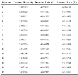
A.1 Red dashed line: Linex loss with a = 1. Blue solid line: EKT loss with p= 2, α= 0.65. . . 112
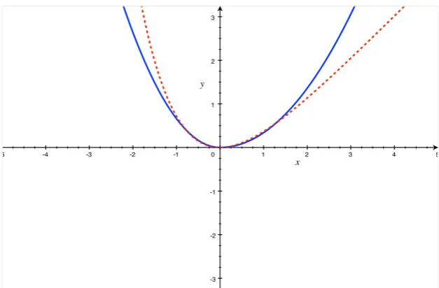
A.2 Red dashed line: Linex loss witha =−1. Blue solid line: EKT loss with p= 2, α= 0.34. . . 112
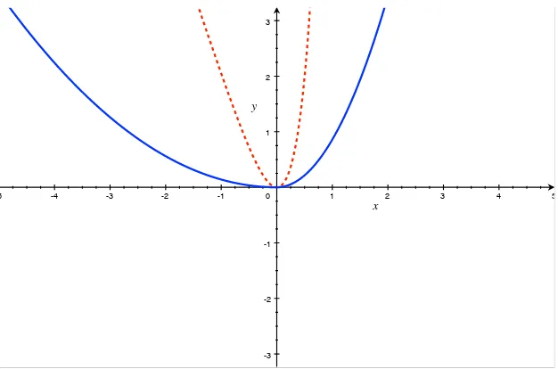
A.3 Red dashed line: Linex loss with a = 3. Blue solid line: EKT loss with p= 2, α= 0.86. . . 113
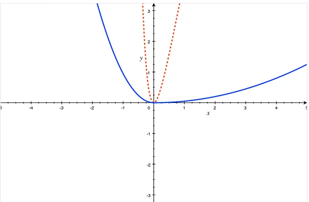
A.5 Red dashed line: Linex loss with a = 5. Blue solid line: EKT loss with p= 2, α= 0.77. . . 114
A.6 Red dashed line: Linex loss witha =−5. Blue solid line: EKT loss with p= 2, α= 0.05. . . 114
C.1 Finite sample densities of the estimator of ζ1 when π0 =−3. . 152
C.2 Finite sample densities of the estimator of ζ2 when π0 =−3. . 152
C.3 Finite sample densities of the estimator of β when π0 =−3. . 153
Acknowledgments
I would like to thank my supervisors: Valentina Corradi, Ana Galvao, Ivana
Komunjer and Jeremy Smith for their continuous encouragement and
sup-port throughout my PhD studies. I am extremely grateful for all their
guid-ance, invaluable suggestions and comments on various previous drafts, and
for always being so helpful. Financial support from the Economic and Social
Research Council as well as the Royal Economic Society is thankfully
ac-knowledged. Part of this thesis was written while the author was visiting the
UCSD Economics Department, whose warm hospitality is gratefully
acknowl-edged. Special thanks to my friends and colleagues, especially: Tina Ammon,
Anna Baiardi, Mahnaz Nazneen, Andis Sofianos, Spyros Terovitis and Raghul
Venkatesh who were a source of constructive discussions and continuous solid
support. Finally, I would like to thank my parents: Elza and Jozsef and my
Declarations
I submit this thesis to the University of Warwick in accordance with the
re-quirements for the degree of Doctor of Philosophy. I declare that this thesis is
my own work and has not been submitted for a degree at another university.
Andrea Anita Naghi
Abstract
Chapter One,A Forecast Rationality Test that Allows for Loss Function
Asymmetries, proposes a new forecast rationality test that allows for asym-metric preferences without assuming any particular functional form for the forecaster’s loss function. The construction of the test is based on the simple idea that under rationality, asymmetric preferences imply that the conditional bias of the forecast error is zero. The null hypothesis of forecast rationality under asymmetric loss (i.e. no conditional bias) is tested by constructing a
Bierens [1982, 1990] conditional moment type test.
Chapter Two, Global Identification Failure in DSGE Models and its
Impact on Forecasting, considers the identification problem in DSGE models and its transfer to other objects of interest such as point forecasts. The re-sults document that when observationally equivalent parameter points belong to the same model structure, the implied point forecasts are the same under both correct specification and misspecification. However, when analyzing the identification problem permitting models with different structures (e.g. dif-ferent policy rules that produce sets of data dynamics that are quantitatively similar), the paper shows that indistinguishable parameter estimates can lead to distinct predictions.
Chapter Three,Identification Robust Predictive Ability Testing,
Chapter 1
A Forecast Rationality Test that
Allows for Loss Function
Asymmetries
1.1
Introduction
The choice of loss function is an important problem in the forecast assessment
literature as it has a direct effect on the results of forecast optimality tests.
Traditionally, empirical studies have based their forecast evaluation framework
on the assumption of a symmetric loss, which implies that positive and negative
forecast errors are equally weighted by the forecaster. Among the symmetric
loss functions, the one that is the most frequently used is the mean squared
error loss, under which forecast efficiency has been studied by testing whether
the forecast errors have zero mean or whether they are uncorrelated with the
available information at the time the forecast was made. A common practice
Theil[1958],Mincer and Zarnowitz[1969] and construct a regression of realized values on a constant and the forecast, testing whether the implied coefficients
are zero and one respectively. Nevertheless, the assumption of a symmetric loss
can be difficult to justify sometimes and often it is not plausible. For example,
at a macroeconomic level, central banks can be averse to bad outcomes such as
lower than expected real output growth and higher than expected inflation and
hence they incorporate this loss aversion into their forecasts. At the level of
individual firms, the cost of under-predicting demand, which results in loss of
sales, should not necessarily be the same as the cost of over-predicting demand,
which means additional storage costs.
Given that symmetric loss functions such as the mean squared error or
mean absolute error may not be flexible enough to capture the loss structures
that forecasters face, another line of the literature (see e.g. Christoffersen and
Diebold [1997], Elliott et al. [2005, 2008] (EKT hereafter), Patton and Tim-mermann [2007a], Patton and Timmermann [2007b], Komunjer and Owyang
[2012]), argues that an asymmetric loss function that weights differently
pos-itive and negative forecast errors could be more representative for the
fore-caster’s intentions. However, under an asymmetric loss, standard properties
of optimal forecast are no longer valid and the traditional forecast rationality
tests could be misleading, not being able to distinguish whether the
forecast-ers use inefficiently their information, or whether the underlying loss function
is just asymmetric. Thus, rejections of rationality in the standard rationality
evaluation literature may largely be caused by the assumption of a squared
loss function. Consequently, this strand of the literature points to the need to
develop testing procedures that are robust to a broader class of loss functions.
Tim-mermann [2007a], established properties of optimal forecasts valid under the
Linex loss function 1 and a popular nonlinear DGP - the regime switching
model ofHamilton[1989]. Patton and Timmermann[2007b] propose tests for
forecast optimality that do not require the knowledge of the specific loss
func-tion, but some testable restrictions have to be imposed on the DGP. Another
framework that is flexible regarding the forecaster’s loss function is the one
inElliott et al. [2005, 2008]. They provide a GMM-based forecast optimality testing framework based on a general class of loss functions that allows for a
parametrization of the asymmetry in the loss and includes the quadratic loss as
a special case. As a by-product of the test, an estimate of the asymmetry
pa-rameter of the loss function is obtained. Komunjer and Owyang[2012] extend
the framework of EKT to a new family of multivariate loss, which by
construc-tion does not impose independence across variables in the loss funcconstruc-tion. The
framework allows for asymmetries in the forecaster’s loss and permits testing
the rationality of a vector of forecasts. More recently, the importance of
eval-uating forecasts under the loss function that is consistent for the functional
of interest (mean, quantile, distribution) has been brought into attention (see
Gneiting[2011],Patton [2014]). For example, if the functional of interest that is forecasted is the mean, the forecasts should be evaluated under the
gen-eral class of Bregman loss functions (Bregman [1967]). Interestingly, under
an asymmetric loss function that belongs to the Bregman class, the optimal
forecast for the mean should not necessarily be biased (see Patton [2014]).
This paper contributes to the literature of forecast assessment under
asymmetric loss. We establish a testable property for forecast rationality that
1The Linex loss function is chosen because it is a popular way to represent asymmetric
holds when the forecaster’s loss function is unknown but it is assumed to be
asymmetric, the framework being also able to accommodate the particular case
when the loss is unknown but symmetric. Our paper is most closely related
to Elliott et al. [2005, 2008]. Unlike Elliott et al. [2005, 2008], our approach accounts for the possibility of asymmetry, without restricting the forecaster’s
loss to any particular parametric form. The attractiveness of our approach
from a practical point of view, is that it can be applied even if the forecast
user does not have any information regarding the shape of the forecaster’s loss
function. Furthermore, we should note that in the construction of our test
statistic, we require neither the knowledge of the underlying loss function nor
the knowledge of the forecasting model used by the forecaster. The forecast
errors required to compute the test could have been generated by a parametric,
nonparametric, semiparametric, or no model at all. The construction of the
proposed test is drawn on the conditional moment tests ofBierens[1982,1990],
De Jong [1996],Corradi and Swanson [2002],Corradi et al. [2009].
Section 1.2 provides a brief review of a commonly used framework for
testing forecast rationality under asymmetry and points out some of its
limi-tations. In Section1.3 we establish a testable property for forecast rationality
under asymmetric loss and outline our proposed test. In Section1.4we present
the advantages of our framework by studying the finite sample properties of our
test under a nonlinear DGP, and emphasizing the effect of a misspecified loss
in the framework of EKT. Section1.5 presents an empirical illustration using
data from the Survey of Professional Forecasters (SPF). Concluding remarks
are provided in Section 2.5. The main simulation and empirical findings are
presented in Appendix A1. Appendix A2 contains additional empirical results
1.2
Testing Forecast Rationality under
Asym-metric Loss: the EKT Framework
Elliott et al.[2005,2008], address the issue of allowing for asymmetric prefer-ences when testing forecast optimality. The forecast rationality test that they
propose is based on a pre-specified class of loss functions that has the following
parametric functional form:
L1 (t+1;p, α) = [α+ (1−2α)·1(t+1 <0)]· |t+1|p (1.1)
This function depends on the forecast error t+1 and the shape parameters
p∈N∗ and α ∈(0,1).
The parameterα describes the degree of asymmetry in the forecaster’s
loss function. This parameter is of important economic interest as it provides
information about the forecaster’s objectives that can be useful for forecast
users. For values of α less than one half the forecaster gives higher weights
on negative forecast errors than on positive ones of the same magnitude, or
in other words over-prediction is more costly than under-prediction. Values
greater than one half indicate a higher cost associated with positive forecast
errors, or that under-prediction is more costly than over-prediction. In the
symmetric case, α equals one half, in which case the costs associated with
positive and negative forecast errors are equally weighted. The relative cost
of a forecast error can be estimated as ˆα/1−αˆ. For example, if the estimated
value of α is 0.75, positive forecast errors obtained by under-forecasting are
three times more costly then negative ones obtained by over-forecasting (see
Special cases of L1 include the absolute deviation loss function
L1(t+1; 1,1/2) the squared error loss functionL1(t+1; 2,1/2) and their
asym-metrical counterparts obtained when α 6= 1/2 - the lin-lin loss L1(t+1; 1, α)
and the quad-quad loss L1(t+1; 2, α). Thus, while this class of loss functions
allows for asymmetric preferences, it also nests the popular symmetric loss
functions widely used in empirical studies.
A sequence of forecasts is said to be optimal under a particular loss
function if the forecast minimizes the expected value of the loss, conditional
on the information set of the forecaster. Elliott et al. [2005, 2008], exploit
the idea that optimal forecasts must satisfy the first order condition of the
forecaster’s optimization problem, and construct a forecast rationality test
based on the following moment conditions:
E(Wt(1(∗t+1 ≤0)−α0)|
∗
t+1| p0−1|
= 0 (1.2)
where ∗t+1 = yt+1−ft∗+1 is the optimal forecast error, the difference between
the realization of some target variable Yt+1 and the optimal forecast, p0 and
α0, are the unknown true values of p and α, and Wt is the information set of
the forecaster.
Using the moment conditions in (1.2), first a GMM estimator for the
asymmetry parameterαis obtained. Then, whether the moment conditions in
(1.2) associated with the first order condition of the forecaster’s optimization
a test for overidentification:
J = 1
T[ T+τ−1
X
t=τ
vt[1(ˆet+1 <0)−αˆT]|eˆt+1|p0−1]0Sˆ−1
[
T+τ−1
X
t=τ
vt[1(ˆet+1 <0)−αˆT]|eˆt+1|p0−1]
(1.3)
The test is asymptotically distributed as a χ2 with d−1 degrees of freedom,
with d the size of the vector of instruments Vt, and rejects for large values.
In (1.3), ˆet+1 is the observed forecast error, τ is the estimation sample size
(in-sample size),T is the number of forecasts available (out-of-sample size), vt
are the observations of the vector of instrumentsVt, ˆαT is a linear instrumental
variable estimator of the true valueα0,
ˆ
αT ≡
[T1 PT+τ−1
t=τ vt|eˆt+1|
p0−1]0Sˆ−1[1
T
PT+τ−1
t=τ vt1(ˆet+1 <0)|eˆt+1| p0−1]
[1
T
PT+τ−1
t=τ vt|eˆt+1|p0−1]0Sˆ−1[ 1 T
PT+τ−1
t=τ vt|eˆt+1|p0−1]
(1.4)
and ˆS, defined as ˆS( ¯αT) ≡ T1
PT+τ−1
t=τ vtv0t(1(ˆet+1 < 0)−α¯T)2|eˆt+1|2p0−2, is a
consistent estimate of a positive definite weighting matrix S, depending on
¯
αT, a consistent initial estimate for α0.
While this approach takes into account asymmetric preferences and
al-lows for a great flexibility regarding the loss function, it relies on a couple
of assumptions. First, it maintains the assumption that the loss function
be-longs to the parametric form given in (1.1). This particular functional form
is substituted in the forecaster’s minimization problem and then the moment
conditions in (1.2) are obtained accordingly. The problem is that if the
fore-caster’s true loss function does not belong to this parametrization, the test
Second, the method is based on the assumption that the forecasts were
generated using a linear model of the type: ft+1 =θ0Wt, where θ is a k-vector
of parameters in a compact set Θ⊂Rk, and thus, the observed forecast error
is: ˆet+1 =yt+1−θˆ0Wt. In this framework, failure to reject the null hypothesis of
rationality, means an absence of linear correlation between the information set
of the forecaster and the forecast error. Hence, possible nonlinear dependencies
are not necessarily detected. The forecast error could be uncorrelated withWt
but correlated with a nonlinear function of Wt. Moreover, the error could be
correlated with some variables not even included inWt. In order to apply this
approach in the case of a nonlinear forecasting rule, ft+1 = f(θ, Wt), Wt in
(1.2) would have to be replaced with the gradient of f with respect to the
parameter θ evaluated at (θ∗, Wt). However, the forecasting model f, its true
parametersθ∗ and Wt are usually not known by the forecast user.
1.3
Forecast Rationality Tests under Unknown
Functional Form of the Loss
In this section, we propose a testable property for forecast rationality under
asymmetric loss and outline a forecast rationality test that can be used when
the forecast evaluator wishes to test for forecast optimality suspecting that
the forecasters give different weights to positive and negative forecast errors.
The proposed test is not based on the assumption of a particular parametric
form for the loss function, the asymmetric preferences being captured in a
non-parametric way. This constitutes an important feature of the test, as the true
evaluation. Another attribute of the test is that it detects possible nonlinear
dependencies between the forecast error and the forecaster’s information set,
therefore it allows for a nonlinear forecasting rule.
To this end, consider first the following null hypothesis
H0 :E(t+1|Wt) = 0 (1.5)
against the alternative
H1 :E(t+1|Wt)6= 0
where t+1 is the forecast error and Wt contains all publicly available
information relevant to predict a variable Yt+1 at time t. If the null in 1.5
is true, it means rationality and unbiasedness of the forecast error, as the
forecast error follows a martingale difference sequence (m.d.s.) with respect
to the information set of the forecaster.
Define now
H0 :E(t+1|Wt) =E(t+1) (1.6)
against
H1 :E(t+1|Wt)6=E(t+1)
The null in (1.6) implies that the conditional expectation of the
fore-cast error equals the unconditional expectation and thus the forefore-cast error is
independent of any function which is measurable in terms of the information
set available at time t. In other words, there is no issue of inefficient use of
is true and E(t+1|Wt) 6= 0 the forecast errors are not only rational but also
biased. Thus, (1.6), under the assumption that E(t+1|Wt) 6= 0, constitutes a
null hypothesis for testing forecast rationality under asymmetric loss.
The null given in (1.6) can be now restated as follows: H0 :E(t+1|Wt)−
E(t+1) = 0 ⇔ H0 : E(t+1|Wt)−E[E(t+1)|Wt] = 0 ⇔ H0 : E[t+1|Wt −
E(t+1|Wt)] = 0 ⇔
H0 :E[(t+1−E(t+1))|Wt] = 0 (1.7)
The alternative of the new form of the null hypothesis can be written as:
H1 :P r [E[(t+1−E(t+1))|Wt] = 0]<1
From the new form of the null hypothesis given in (1.7), it can be seen that
test-ing for forecast rationality under asymmetric loss, reduces to testtest-ing whether
the quantity E[(t+1 −E(t+1))|Wt], i.e. the conditional bias of the forecast
error, is zero.
We are now able to construct a Bierens [1982, 1990] type test for the
null given in (1.7).
To this end, we apply to our context the test statistic suggested by
De Jong [1996] which generalizes the consistent model specification test
pro-posed byBierens [1990], to the case of data dependence. Thus, we define:
where:
mT(γ) =
1
√ T
T−1
X
t=0
(ˆet+1−e)w
t−1
X
j=0
γj0Φ(Wt−j) !
(1.9)
Exploiting the equivalence E[(t+1 −E(t+1))|Wt] = 0 ⇔ E[(t+1 −
E(t+1))w(γ0, Wt)] = 0, consistent model specification tests are based on the
discrepancy of the sample analog of E[(t+1 −E(t+1))w(γ0, Wt)] to zero. In
(1.9), ˆet+1 is the observed one-step ahead forecast error obtained as the
differ-ence between the actual realization and the forecasted value from the forecast
producer, ˆet+1 =yt+1−fˆt+1. The mean e is defined as e= T1
PT−1
t=0 eˆt+1, and
T is the number of observed forecast errors. Our discussion focuses on ˆet+1,
but the results generalize to ˆet+h, whereh >1 is the forecast horizon.
The function w(γ0, Wt) is a generically comprehensive function, a
non-linear transformation of the conditioning variables. Commonly used functions
in the literature for w are: w(γ0, Wt) = exp(
Pk
i=1γiΦ(Wi,t)), or w(γ
0, W
t) =
1/(1 + exp(c−Pk
i=1γiΦ(Wi,t))), where c is a constant, c 6= 0, and Φ is a
measurable one-to-one mapping from R to a bounded subset of R, it can be
chosen the arctangent function, for example. The choice of the exponential
in the weight function w is not crucial. Stinchcombe and White [1998] show
that any function that admits an infinite series approximation on compact sets
with non-zero series coefficients can be used to obtain a consistent test. The
weights,γj, attached to observations decrease over time.
The following remarks are worth making at this point.
Remark 1. In the particular case in which forecast efficiency is tested under
a symmetric loss function, one can testH0 :E(t+1|Wt) = 0, which if it is true
to the information set used by the forecaster. The test statistic thus becomes:
MT =supγ∈Γ|mT(γ)|, withmT(γ) = √1T PT
−1
t=0 eˆt+1w
Pt−1
j=0γ
0
jΦ(Wt−j)
.
Remark 2. Suppose now that the true loss function is asymmetric and one
uses MT =supγ∈Γ|mT(γ)|, with mT(γ) = √1T
PT−1 t=0 eˆt+1w
Pt−1
j=0γ
0
jΦ(Wt−j)
to test for forecast rationality, then this form of the test might falsely reject
rationality as it is based on the assumption of a symmetric loss.
The proposed test statistic has a limiting distribution that is a
func-tional of a Gaussian process (see e.g. Corradi et al. [2009]). Under H0,
MT d
→ supγ∈Γ|mT(γ)|, where m(γ) is a zero mean Gaussian process.
Un-der H1, there exist an > 0, such that: P r
1
√
TMT >
→ 1. The proof
follows from the empirical process CLT of Andrews [1991], for heterogeneous
near-epoch dependent (i.e. functions of mixing processes) arrays. The limiting
distribution of the statistic,MT is the supremum over a Gaussian process and
hence standard critical values are not available. Also, note that MT is not
pivotal because the limiting distribution depends on the nuisance parameter
γ ∈ Γ. The test has power against generic nonlinear alternatives, but the
critical values have to be computed by bootstrap. In the Monte Carlo study
and the empirical part of the paper, the block bootstrap is employed to obtain
the critical values for the test. In the block bootstrap, ˆet+1 and the data are
jointly resampled in order to preserve the correct temporal behavior and to
mimic the original statistic.
1.4
Monte Carlo Evidence
Our Monte Carlo study consists of two parts. First, we emphasise the
illustrate the effect that a misspecified loss function can have in the forecast
evaluation framework of EKT. Then, we compare the empirical power of our
proposed test with that of the J-test, in the presence of nonlinear
dependen-cies between the sequence of forecast errors and the information set available
at the time the forecast is made.
1.4.1
The Effect of a Misspecified Loss Function in
Fore-cast Evaluation
We illustrate the loss function sensitivity of the EKT framework, by
construct-ing a Monte Carlo exercise where the forecaster’s true loss function does not
belong to the class of loss functions on which the test is based on. Nevertheless,
the forecast evaluation is done under the particular class of loss introduced in
EKT. To highlight the effect of a misspecified loss function, we examine the
behavior of the estimator ˆα and study the properties of theJ-test.
We assume that the variable of interest is generated by a simple AR(1)
process:
Xt=b+cXt−1+t
where the errors are serially uncorrelated,t ∼N (0, 0.5), and the parameters
are set to b = 0.9 and c = 0.7. We generate random samples of size T =
R+P −1, after discarding the first 100 observations to remove initial values
effects. Using a rolling window of size R, the forecaster constructs P one
period ahead forecasts by minimizing the expected value of the loss function,
forecast is thus ˆft+1,t= ˆb+ ˆcXt where ˆb and ˆcare obtained by minimizing L1:
(ˆb,cˆ) = arg min R−1
R X
t=1
L1 (α0, Xt+1−b−cXt) (1.10)
whereα0 is the true value of the forecaster’s loss function asymmetry
param-eter. The sequence of the observed forecast errors is then computed as:
{ˆet+1}Tt=R={Xt+1−ˆb−cXˆ t}Tt=R
We perform 1000 Monte Carlo simulations for different choices ofR,P andα0.
The instrument set in this section includes a constant and the lagged forecast
errors.
TableA.1reports the average α0 estimates for various sample sizes and
various values of the true asymmetry parameter. As expected, the estimator
performs overall well when the loss function is correctly specified, the
esti-mated values being close to the true values. Table A.2 reports the empirical
rejections probabilities for theJ-test. Under a correctly specified loss, size is
well controlled. There are some size distortions in cases when the in-sample
size is smaller or equal to the out-of-sample size, indicating the importance of
controlling the relative sizes of R and P.
Now, we examine the implications of falsely assuming that the
fore-caster’s true loss function belongs to (1.1). We reconstruct our Monte Carlo
exercise assuming now that the forecaster’s true loss function is the Linex loss
and exponential terms and it is defined as:
L2(t+1;a) = exp(a·t+1)−a·t+1−1 (1.11)
This time, the forecast evaluation is done inaccurately under the loss function
given in (1.1). In this case, ˆb and ˆc are obtained as:
(ˆb,cˆ) = arg min R−1
R X
t=1
L2 (a0, Xt+1−b−cXt)
wherea0 is the true value of the Linex loss function’s asymmetry parameter.
TableA.3reports the average GMM estimates ofα for different sample
sizes and different values of the Linex loss function’s true asymmetry
param-eter. The average estimates present large variations across different values of
the true loss function’s asymmetry parameter, and they are far from the true
values. The results given in TableA.4indicate the size distortions of theJ-test
obtained when the forecast evaluation is done under a misspecified loss
func-tion. TheJ-test tends to over reject the null of rationality, the size distortions
being larger for larger values (in absolute value) of the Linex loss function’s
asymmetry parameter. The size distortions seems to be smaller though in
cases where the Linex loss function’s parameter is closer to the origin.
In order to better understand when the J-test suffers from size
distor-tions, figures A.1 to A.6, plot the EKT and the Linex loss functions on the
same graph with different parametrizations. Take for example Figure A.1.
Here, the Linex loss function’s parameter,a, is fixed to 1 while the EKT loss
function’s parameters arep= 2 andα= 0.65 - the incorrectly estimated value
Under these parametrizations, the two loss functions overlap on a notably large
region and the rejection frequencies for the J-test, under a misspecified loss
function, (as obtained in TableA.4), are not that far from the nominal level of
5%. FigureA.3, shows a case when the two functions have only a very small
overlapping region at the origin. In this graph, a = 3, p = 2 and α = 0.86.
When the common region of the two functions is small, the J-test does not
control size well and leads to over rejections of the null of rationality.
1.4.2
Empirical Size and Power Comparison
In the second Monte Carlo setup, we consider the following data generating
process:
Yt=θ0Wt+δg(φ0Wt) +Ut (1.12)
where θ0 = (θ1, θ2), φ0 = (φ1, φ2) and Wt = (W1t, W2t)0. We set the
fol-lowing expressions for the nonlinear function g, g(x) = x2, g(x) = exp(x),
g(x) = arctan(x). Different parametrization are set for δ, the parameter
that quantifies the size of the nonlinearity, as indicated in Table A.5. The
parameters governing the process, θ and φ, are fixed to (θ1, θ2) = (0.5,0.5),
(φ1, φ2) = (0.7,0.8). In this section, the instrument set is a constant and Zt
- which is generated such that it is correlated withW1t, W2t but uncorrelated
multivari-ate normal distribution:
W1t
W2t
Zt
Ut
∼N(0,Σ)
where Σ is the variance-covariance matrix set to:
Σ =
2 0.1 0.8 0.2
0.1 2 1 0.1
0.8 1 2 0
0.2 0.1 0 0.8
We generate a sample of size T = 500 for Yt according to the data
generating process given in 1.12. We assume the forecaster uses the first
R= 0.6×T observations to estimate the parameters of a linear model:
Yt =θ1W1t+θ2W2t+Ut
The sequence of one-step ahead forecasts, ˆYt+1 = ˆθ1W1t + ˆθ2W2t, and the
observed one-step ahead forecast errors ˆet+1 are obtained using a recursive
scheme. Given that a linear forecasting model was used to generate the forecast
errors even though the data was generated by a nonlinear process, we ensure
that the resulting forecast error is correlated with some nonlinear function of
Wt. This means that whenever δ 6= 0, we can study the empirical power of
the tests, while when we setδ to 0, we obtain the empirical sizes. We perform
Carlo simulation we perform 100 bootstrap simulations in order to obtain the
critical values for theMT statistic.
Table A.5 reports the rejection frequencies at a 10% significance level
for different nonlinear functions, g(x), and for different parametrization for
δ. When we set δ = 0, the forecast error is uncorrelated with the available
information and both tests have an empirical size close to the nominal size of
10%. In all the other cases characterized by a nonlinear relationship between
the forecast error and the information set, theMT test outperforms theJ-test.
1.5
Empirical Illustration
In this section, we perform an empirical comparison of the MT and J tests
using data from the Survey of Professional Forecasters (SPF) maintained by
the Federal Reserve Bank of Philadelphia. In this data set, survey participants
provide point forecasts for macroeconomic variables in quarterly surveys. As
the objective of the forecaster is unknown, it is not sure that the forecaster
simply minimizes a quadratic loss function and reports the conditional mean.
Thus, when evaluating these forecasts, it is reasonable not to impose too much
structure on the unknown loss function. Nevertheless, the reported forecasts
should indeed reflect the underlying loss function.
The following series were selected for this empirical application:
quar-terly growth rates for real GNP/GDP (1968:4-2012:4),2 the price index for
GNP/GDP (1968:4-2012:4), and the quarterly growth rates for consumption
(1981:3-2012:4).3 The growth rates are calculated as the difference in natural
logs. For robustness, we perform our analysis on median, mean and range
forecasts. Results on the median mean and range forecasts are provided in
Appendix A.
In the computation of the two statistics, we considered the one-step
ahead forecast error obtained as the difference between the actual and the
one-step ahead forecasted value. The point forecast data set of the SPF provides
data on the year, the quarter, the most recent value known to the forecasters,
the value for the current quarter (which is usually forecasted) and then
fore-casts for the next four quarters. To compute the one-step ahead forecasted
growth rates, we used values corresponding to the current quarter and the
most recent known value. For the actual values, the SPF provides a real-time
data set. In order to compute the actual growth rates we used the first release.
For the instruments of the J-test and the information set used in the
computation of the MT test, we considered the following six cases: Case 1
-constant and lagged errors, Case 2 - -constant and absolute lagged errors, Case
3 - constant and lagged change in actual values, Case 4 - constant and lagged
change in forecasts, Case 5 - constant, lagged errors and lagged change in
actual values, Case 6 - constant, lagged errors, lagged change in actual values
and lagged change in forecasts.
In the construction of theMT statistic we adopt commonly used settings
in the literature. We chose the exponential function forw and the arctangent
function for Φ. Also, we set γj ≡ γ(j + 1)−2, where γ ∈ [0,3] when γ is
example for Case 5:
γ =
γ1
γ2
γ3
∈[0,3]×[0,3]×[0,3]
and the test statistic is computed as the supremum of the absolute value of:
mT(γ) =
1
√ T
T−1
X
t=0
(ˆet+1−e) exp
"t−1 X
j=0
(γ1(j+ 1)−2tan−1(Z1,t−j)
+γ2(j+ 1)−2tan−1(Z2,t−j) +γ3(j+ 1)−2tan−1(Z3,t−j))]
(1.13)
where Z1 is a vector of ones, Z2 contains the lagged errors andZ3 the lagged
change in actual values. The critical values for the MT test, are computed
using the block bootstrap with blocks of length 5 and an overlap length of
2. Given the small sample sizes, we derive our conclusions based on the 10%
bootstrap critical values.
Table A.6 reports the results obtained for the J-test based on the
median forecasts. The estimates of the asymmetry parameter for the real
GNP/GDP take values slightly less than 0.5, while for the price index the
estimates take values slightly higher than 0.5. However, when performing at
-test that -testsH0 :α= 0.5, the null of symmetric preferences, in the context of
the EKT class of loss, cannot be rejected for GNP/GDP and the price index.
Interestingly, this null hypothesis is rejected for consumption - variable for
which forecasters tend to under-predict. At the 10% level, theJ-test does not
reject the composite null hypothesis that the loss belongs to the family of loss
and the price index. However, it does reject for most instrument set cases of
consumption - specifically for Cases 1, 3, 5 and 6.
Analyzing now Table A.7, where our suggested nonlinear test is
com-puted, we notice that for the real GNP/GDP, our test results are in conformity
with theJ- test’s results - forecast rationality is not rejected for this variable.
We obtain however contrasting results that reveal interesting insights for the
price index and consumption. Unlike the J-test, the MT test rejects forecast
rationality for the price index, which suggests that in the case of inflation, the
forecast error depends in a nonlinear fashion on the information set used to
produce the forecasts and theJ-test is not able to detect these nonlinear
de-pendencies. For consumption, our test does not reject rationality, even though
the J-test rejects the null. This might be an indication that the true loss
function used to generate the forecasts for consumption was from a different
family of loss than the one theJ-test is based on, and consequently theJ-test
cannot distinguish whether the forecasters use inefficiently their information
or whether the underlying loss function does not belong to the pre-specified
loss, and therefore it rejects the null.
The empirical results on the mean and the range responses confirm our
results on median forecasts. The results on these two series are included in
Appendix A.
1.6
Conclusion
In this paper, we propose a new forecast rationality test that allows for
asym-metric preferences, without assuming a particular functional form for the
fore-cast rationality under an asymmetric loss function implies a zero conditional
bias of the forecast error. Our framework is based on the classical literature
on consistent model specification tests in the spirit of Bierens [1982, 1990],
De Jong[1996]. The asymmetry in the loss function is captured in a
nonpara-metric way. The drawback of the latter is that in contrast to Elliott et al.
[2005, 2008], this approach cannot quantify the magnitude of the asymmetry
in the loss function, which can be of important economic interest.
Monte Carlo simulations illustrate the advantages of our approach. We
show that a commonly used test that accounts for the possibility of asymmetric
preferences is loss function sensitive and may lead to incorrect inference if the
loss function is misspecified, whereas our test can be used without requiring
the specification of a particular functional form for the loss. In addition,
simulations show that our proposed test has good finite sample properties
even when the forecasting rule is nonlinear.
Our empirical study highlights some differences in the results that we
obtain when applying the two forecast rationality tests to data from the Survey
of Professional Forecasters. The contradiction in the results reveal interesting
Chapter 2
Global Identification Failure in
DSGE Models and its Impact
on Forecasting
2.1
Introduction
Dynamic stochastic general equilibrium (DSGE) models use a coherent
the-oretical framework to understand and explain macroeconomic fluctuations.
Important policies are routinely produced based on the estimates of DSGE
parameters. Before performing an empirical analysis with a particular model,
it is essential however that the model be checked for identifiability. Assessing
the identifiability of DSGE models is important for both econometric rigour
as well as for delivering reliable policy recommendations. On the one hand,
a parameter that is not identifiable cannot be consistently estimated.
Identi-fication issues can lead to misleading estimation and inference. On the other
can be distinct, the reliability of policy recommendations depends upon the
primitive assumption of identifiability.
Although the validity of statistical inference in DSGE models has been
questioned due to identification deficiencies (see for e.g. Beyer and Farmer
[2004],Canova and Sala[2009]), there are relatively few papers in the literature that assess the impact of identification failure on different macroeconomic
outcomes 1. The purpose of this paper is to examine whether the fragility
of parameter estimates in DSGE models, resulted from lack of identification,
transfers to other objects of interest such as point forecasts. A few papers
in the literature analyzed the effect of identification loss on impulse response
functions (see for e.g. Morris [2014]), but to my knowledge no existing paper
examines the impact of identification failure on forecasting with DSGE models.
In this paper, we focus onglobal identification failure, as this particular
identification issue is of interest when giving policy recommendations based
on DSGE models. Other types of identification failures such as local and
weak identification, even though interesting from the point of view of the
econometric challenges that they imply, they are less relevant from a policy
perspective. We illustrate the results through the model ofAn and Schorfheide
[2007], a small scale DSGE model, representative for the models currently used
in monetary policy analysis at policy institutions. This particular model has
been chosen for the analysis motivated by the fact that the dimension of the
parameter space is not too large and thus, it permits the computation of the
numerical results in reasonable times.
As there are currently no available analytical results for global
identifi-cation in DSGE models, we proceed by assessing global identifiability
ically. To this end, we construct a fine grid on the economically meaningful
parameter space, for the starting values used in the optimization of the
objec-tive function. Using these starting values, the aim is to find through a global
optimization algorithm, severaldistinct maximizing parameter values yielding
the same value for the likelihood. In searching for observationally equivalent
points, we treat two cases: optimizing the log-likelihood (frequentist approach)
and optimizing the log-posterior (Bayesian approach).
We show numerically that when the model is solved with linear
approx-imations, three parameters: the inverse elasticity of demand (ν), the price
stickiness (φ), and the steady state of government spending (1/g) fail to be
globally identified. In contrast, under nonlinear approximations, where
second-order accurate solutions to the DSGE model are obtained from a second second-order
expansion of the equilibrium conditions, these three parameters become
glob-ally identifiable. This sheds some light on a scarcely investigated issue in the
literature: the log-linearization error in DSGE identification. The reason why
in this particular model, quadratic approximations can identify the structural
parameters that are not identifiable under the log-linearized model is that ν
and φ become linearly independent in the nonlinear version of the Philips
curve, and g does appear in the nonlinear equilibrium equations, while it did
not enter the linear likelihood. These findings confirm the hypotheses made
inAn and Schorfheide [2007], based on likelihood contour graphs.
Based on observationally equivalent parameter points obtained from the
grid search results, we perform several forecasting exercises: i) forecasting with
observationally equivalent parameter values from a correctly specified model,
ii) forecasting with observationally equivalent parameter values from
arising from different model structures. The focus here is on the linear model
only, where there is evidence for global identification failure.
The results show that when observationally equivalent parameter
es-timates belong to the same model structure, they imply the same system
matrices, which result in the same point forecasts, under both correct and
misspecification. Thus, global identification failure does not impose issues
in constructing predictions from DSGE models, when identification is
condi-tional on the model structure, i.e. in a framework where there could exist
different parameter values within the same DSGE structure that lead to the
same dynamics of the observables. However, when the identification problem
is analyzed permitting different structures, (e.g. models with different policy
rules, different types of frictions or shock processes), two parameter points
that generate the same data dynamics can lead to distinct forecasts. This is
illustrated with observationally equivalent parameter estimates arising from
two model structures: one in which the monetary policy follows an interest
rate rule that reacts to current inflation, and another where the central bank
responds to expected inflation. The differences in the obtained forecasts can be
large. With a current inflation specification, the forecasted quarter-to-quarter
GDP growth rates are around -0.5% and the annualized quarter-to-quarter
inflation rates are around 2.8%, while with an expected inflation specification,
the quarter-to-quarter GDP growth rates are around 1.9% and the annualized
2.1.1
Related Literature
The paper is related to two main strands of literature. The first line
con-cerns the literature on DSGE identification - which is by now fast growing.
One of the first papers that draw attention to the identification problems in
these models was Canova and Sala [2009]. They suggest several diagnostic
procedures for identification based on graphical and simulation analyses.
A couple of papers made advances in providing formal conditions for
local identification. Iskrev [2010] obtains sufficient (but not necessary) con-ditions for local identification based on the rank of the Jacobian matrix that
maps the deep parameters to first and second moments of the observables. His
approach is suitable when the DSGE model is estimated by likelihood based
methods. Komunjer and Ng [2011] establish rank and order conditions for
local identification from restrictions implied by equivalent spectral densities
for both singular2 and non-singular models. Their established conditions are
independent of the data or the estimator used and can be verified prior to
esti-mation. Qu and Tkachenko[2012] obtain necessary and sufficient condition for
local identification formulated in the frequency domain. Related to nonlinear
DSGE models, Morris and Lee [2014] provide rank and order conditions for
local identification of parameters in nonlinear models.
Another stream of literature focuses on the issue of global
identifica-tion. Fukaˇc, Waggoner, and Zha[2007] study global identification in invertible
DSGE models, with solutions in a VAR form. Qu and Tkachenko [2013]
in-troduce a criterion based on the Kullback-Leibler distance between two DSGE
models computed in the frequency domain and shows that global identification
fails if and only if the criterion equals zero when minimized over the relevant
region of the parameter space. They consider log-linearized DSGE models, and
treat both determinacy and indeterminacy 3 cases, the results being
applica-ble for singular and non-singular models. Basing their analysis on the time
domain, Kociecki and Kolasa [2014] obtain a necessary (order) condition for
global identification and develop an efficient algorithm that checks for global
identification by shrinking the space of admissible parameter values. The last
two approaches for checking global identification in DSGE models are
(compu-tationally intensive) numerical methods and the literature still lacks complete
formal analytical conditions for global identification. The above mentioned
pa-pers examine identification of the DSGE system as a whole. An earlier strand
of the literature raised questions about identification of particular equations in
a DSGE model such as the Philips curve: Mavroeidis [2005], Kleibergen and
Mavroeidis[2009] or the Taylor rule: Cochrane [2011]
Related to the problem ofweak identification 4in DSGE models, several
inference methods robust to weak identification have been proposed. These
methods are all based on the inversion of test statistics. Andrews and
Miku-sheva[2014] focus on testing and confidence set construction using two weak identification-robust forms of the classical LM test. Working in the frequency
domain, Qu[2014] develops asymptotically valid confidence sets for the
struc-3Indeterminacy appears when the log-linearized models has multiple solutions. In this
case, the state-space representation is not uniquely determined by the model because the variables that enter the state transitions equation as well as the matrices that appear in the transition equation differ according to the solution of the model.
4When a DSGE model is weakly identified, the likelihood function is not completely flat,
but has very low curvature with respect to some parameters. Weak identification causes statistics to be non-normally distributed even in large samples. Also, as illustrated in
Guerron-Quintana et al.[2013], the usual asymptotic equivalence results between Bayesian
tural parameters and uniform confidence bands for the impulse response
func-tions. Dufour, Khalaf, and Kichian [2013] propose a limited information
ap-proach and suggest the inversion of moment based tests, the apap-proach
be-ing applicable to DSGE models that have a finite order VAR representation.
Guerron-Quintana, Inoue, and Kilian[2013] construct confidence sets that re-main asymptotically valid when the structural parameters are weakly identified
by inverting the likelihood ratio statistic and the Bayes factor. A test that
detects weak identification is proposed in Inoue and Rossi [2011]. They
im-plement their approach to test the null of identification against weak (or no)
identification of the structural parameters in a Taylor rule monetary policy
reaction function.
More recently, the literature started to exploittime variation in
param-etersas a source of identification. Magnusson and Mavroeidis[2014] show that time variation in a subset of parameters can be used in the identification of
parameters that are stable overt time. Canova et al.[2015] illustrate that
iden-tification problems in DSGE models may arise as a result of misspecification
due to neglected parameter variation. In a related literature that focuses on
testing the correct specification of DSGE models, Komunjer and Zhu [2016],
highlight that the parameters (system matrices) of the DSGE’s state space
model representation are not identified, and construct a likelihood ratio test,
using classical testing theory, for the validity of the DSGE model, taking into
account this lack of identification.
The second main strand of literature this paper is related to, is the
literature on forecasting with DSGE models. These models have become by
institutions. The particular interest in forecasting with theoretically-grounded
DSGE models among policy institutions, is motivated by the fact that
com-pared to a-theoretical models (such as VARs, BVARs or DFM), DSGE models
have a high degree of theoretical coherence, they deliver a richer
interpreta-tion of the results, and can be used to construct predicinterpreta-tions on the effects of
alternative policy scenarios.
The forecasting performance of DSGE models has been shown to be
competitive with alternative prediction methods used at central banks. Results
from the seminal papers Smets and Wouters [2003] and Smets and Wouters
[2007] suggest that DSGE model based forecasts compare well with forecasts
obtained from reduced form models such as standard and Bayesian VARs.
Similar results have been obtained byEdge, Kiley, and Laforte[2010]
compar-ing the FRB’s DSGE model to alternative reduce-form time series models, the
Greenbook forecasts and the FRB/US model forecasts. The forecasting
per-formance of DSGE models for the Euro area has been assessed byChristoffel,
Coenen, and Warne [2010] (paper uses the NAWM model developed at the
ECB) and Adolfson, Lind´e, and Villani [2007b]. The forecasting accuracy of
the Riksbank’s DSGE model has been evaluated by Adolfson et al. [2007a].
All these studies differ in terms of the estimation sample, forecasting
sample, variable definitions or data vintages used. In order to make the DSGE
forecasting performance results comparable across different studies, in a survey
paper,Del Negro and Schorfheide[2013] compute the ratio between the RMSE
reported in various papers and the RMSE of a benchmark AR(2) model.
Over-all, they find that in terms of forecast accuracy, DSGE models compare well
with alternative prediction methods - especially for the output growth and
Nevertheless, some authors bring critiques on the forecasting
perfor-mance of DSGE models (see for e.g. Giacomini[2014],Gurkaynak et al.[2013],
Giacomini and Rossi[2012] ). They emphasize that the conclusion reached by the aforementioned studies is sensitive to arbitrary choices that one makes
(such as the choice of the observables, the choice of the priors and
hyperpa-rameters, data processing such as detrending, or how one deals with stochastic
singularity), when assessing the forecasting performance of DSGE models.
Beyond forecasting with standard DSGE models, another strand of
liter-ature, focuses on obtaining forecasts combining DSGE models with VARs (see
e.g. Del Negro and Schorfheide[2004],Amisano and Geweke[2013],Waggoner and Zha[2012]) or with DFM (see e.g. Schorfheide, Sill, and Kryshko [2010]; incorporating external information into DSGE model based forecasts such as
nowcasts, expectations on inflation, output and interest rate (Del Negro and
Schorfheide[2013]); or incorporating theoretical restrictions into a-theoretical
models using exponential tilting (Giacomini and Ragusa [2014]).
Section2.2 sets up the econometric framework and presents the
speci-ficities of the identification problem in DSGE models. Section 2.3 illustrates
numerically the failure of global identification in a small scale prototypical
DSGE model. The model is analyzed in both log-linear and nonlinear form.
Several forecasting exercises based on observationally equivalent parameter
2.2
The Identification Problem in DSGE
Mod-els
In this section, we introduce the ABCD representation of a DSGE model,
present the particularities of the model that make the classical identification
results inappropriate in this framework and highlight the implications of
iden-tification failure in both the classical and Bayesian estimation approaches.
2.2.1
Setup
Consider a DSGE model with structural parameters θ belonging to a set Θ⊆
Rnθ. Let X
t be an nX ×1 state vector, Yt an nY ×1 vector of observables
and t a vector of structural shocks of size n ×1. After writing down the
system of nonlinear expectational equations of the model, a solution to it can
be obtained, which will have the form given in (2.1).
Xt=f(Xt−1, t, θ) (2.1)
The state transition equation (2.1) is pinned down by either finding a close
form expression for the functionf(·), or more frequently, by numerical
approx-imation5. The majority of the literature focuses however on the log-linearized
model around the steady-state, in order to work with a linear version of the
state transition equation:
Xt=AXt−1+Bt (2.2)
5Several solution algorithm are available, such as: Uhlig et al.[1999],Klein[2000],
where the matrices A and B are nonlinear transformations of the structural
parameter θ. In order to compute a likelihood for the DSGE model, a set of
observable variables Yt has to be chosen and a measurement equation such as
(2.3) specified.
Yt=CXt−1+Dt (2.3)
The matrices C and D depend nonlinearly on θ. Equations (2.2) and (2.3)
form the state-space representation or (ABCD representation) of the model:
Xt |{z} nX×1
= A
|{z} nX×nX
Xt−1
| {z } nX×1
+ B
|{z} nX×n
t |{z}
n×1
Yt |{z} nY×1
= C
|{z} nY×nX
Xt−1
| {z } nX×1
+ D
|{z} nY×n
t |{z}
n×1
(2.4)
If the state-space representation is linear such as (2.4), it can be estimated
using the Kalman filter. For nonlinear state space models, typically the particle
filter (see for e.g. Pitt and Shephard[1999]) is used. The ABCD representation
of the model constitutes the starting point of most of the analysis in the
literature and has a central roll when discussing identification in DSGE models.
2.2.2
Definitions
Identification problems in DSGE models arise when different values of the
structural parameters lead to the same joint distribution of the observables. In
other words, changes in some of the parameters may result in indistinguishable
outcomes.
defini-tions related to the problem of identifiability in the context of DSGE models,
(Rothenberg [1971]).
Definition 1. Given a nY ×1 vector of observed data Y, a nθ ×1 vector
of DSGE structural parameters of interest θ ∈ Θ ⊆ Rnθ and the likelihood
functionL(θ;Y), two parameter points of a DSGE modelθ0 and θ1 belonging
to the set Θ ⊆ Rnθ are said to be observationally equivalent if L(θ
0;Y) =
L(θ1;Y) for all Y.
Remark 3. Note that the concept of observational equivalence is not
re-stricted to a particular sample. In other words, two points are observationally
equivalent if the likelihood function evaluated at these two points has the same
value, regardless of the data set used.
This work considers howeversample observational equivalence, because
in practice, when a researcher estimates a DSGE model and faces the problem
of identification failure, she works with a particular data set.
Remark 4. In a Bayesian setup too, observational equivalence reduces to the
equality of the likelihoods.
Definition 2. A DSGE model is locally identifiable at a point θ0 ∈Θ if there
exist an open neighborhood of θ0 such that for everyθ1 in this neighborhood,
θ0 and θ1 are observationally equivalent if and only if θ0 =θ1.
Definition 2 states that a parameter point is locally identified when it
is uniquely distinguishable in an -neighbourhood. Local identification is a
necessary condition for well behaved estimators to exist, in the sense of having
a well behaved distribution. Establishing local identifiability is useful if it is
product of interest. As pointed out in Komunjer and Ng [2011], even if a model is locally identified at every point in the parameter space, it can still
fail to be globally identified.
The main focus of this paper is on global identification.
Definition 3. A DSGE model isglobally identifiable at a pointθ0 ∈Θ if there
is no other θ1 in the parameter space Θ that is observationally equivalent to
θ0.
Global identification deals with the question of whether there exists
an-other point in the parameter space that results in the same macroeconomic
dynamics: autocovariances, impulse responses. This is a question of
inter-est for economists, because if the model is not globally identified, there exist
multiple likelihood maximizing parameter values in the admissible parameter
space, which can have important consequences on quantitative policy
analy-sis, forecasting or scenario simulations. For example, a recent work byMorris
[2014], documents the effect of a multiplicatively-valued maximum likelihood
estimator on monetary policy impulse responses. He shows that
observation-ally equivalent parameter points can lead to distinct monetary policy impulse
responses and thus yield different macroeconomic consequences.
2.2.3
Non-identifiability of the ABCD matrices
Finding analytical conditions for identification in DSGE models has proven
to be a difficult problem for several reasons. First of all, compared to
lin-ear simultaneous equations, identification in DSGE models is less
transpar-ent because the system matrices of the state-space represtranspar-entation are highly
evalu-ated numerically. Secondly, the classical identification results for simultaneous
equations such asFisher[1966],Koopmans[1950],Rothenberg[1971] are valid
only for static models, while DSGE models are dynamic by construction.
Per-haps the most important reason why the classical identification results fail in
the case of DSGE models is that the rank conditions from Rothenberg [1971]
6 are based on the assumption that the reduced form parameters are
identifi-able, an assumption that is not verified in the case of DSGE models. Thus,
the classical approach of identifying structural parameters from reduce form
parameters cannot be applied as the state-space solution is not a standard
reduced form. To see this, consider the following result that characterizes
observational equivalence in singular systems.
Proposition 1. (Komunjer and Ng[2011]): Observational Equivalence,n ≤
nY
Under Assumptions 1, 2, 4S and 5S from Komunjer and Ng [2011], θ0
andθ1 are said to be observationally equivalent if and only if there exists a full
rank nX ×nX matrix T and a full rank n×n matrix U such that:
A(θ1) = T A(θ0)T−1
B(θ1) = T B(θ0)U
C(θ1) =C(θ0)T−1
D(θ1) = D(θ0)U
Σ(θ1) =U−1Σ(θ0)U−1
0 .
(2.5)
6Rothenberg[1971] shows that a parameter is identified at a pointθ
0, if the information
Proposition (1) is used to derive formal identification (rank and order)
conditions for the structural parameters θ. The immediate implication of
Proposition (1) is that the ABCD matrices are not identified. To clarify this,
start from the state space representation of the model:
Xt =A(θ)Xt−1+B(θ)t
Yt=C(θ)Xt−1+D(θ)t
Multiply byT the transition equation to get:
T Xt=T A(θ)Xt−1+T B(θ)t
which is equivalent to
T Xt =T A(θ)T−1T Xt−1+T B(θ)U U−1t
that can be written as
T Xt |{z}
f
Xt
=T A(θ)T−1
| {z }
]
A(θ)
T Xt−1
| {z }
^
Xt−1
+T B(θ)U
| {z }
]
B(θ)
U−1t | {z }
e
t
Analogously, the measurement equation can be written as:
Yt=C(θ)T−1T Xt−1 +D(θ)U U−1t
or
Yt=C(θ)T−1
| {z }
]
C(θ)
T Xt−1
| {z }
f
Xt
+D(θ)U
| {z }
]
D(θ)
U−1t | {z }
e