Control of large offshore wind turbines

(1)

A Thesis Submitted for the Degree of PhD at the University of Warwick

Permanent WRAP URL:

http://wrap.warwick.ac.uk/99841/

Copyright and reuse:

This thesis is made available online and is protected by original copyright.

Please scroll down to view the document itself.

Please refer to the repository record for this item for information to help you to cite it.

Our policy information is available from the repository home page.

(2)

Control of Large Offshore Wind Turbines

by

Xin Tong

Thesis

Submitted to the University of Warwick in partial fulfilment of the requirements for the degree of

Doctor of Philosophy

School of Engineering

(3)

List of Tables

2.1 Selected gross properties of the NREL offshore 5-MW baseline wind turbine model. . . 22 2.2 Undistributed properties of the NREL OC3 monopile 5-MW wind

turbine tower. . . 23 2.3 Distributed properties of the NREL OC3 monopile 5-MW wind

tur-bine tower [1]. . . 23 2.4 Selected tower and barge properties of the NREL ITI Energy barge

5-MW wind turbine model. . . 24 4.1 Values of the H2-norm (4.50) of Σd withN increasing from 9 to 17. 62

(7)

4.3 The optimal parameters of 9 TMD systems and the values of cor-responding objective functions fhc (4.101) and fh (4.105) at these

optimal parameters (all denoted by superscript∗ ) for the SCOLE-TMD system under harmonic excitations. q is the number of TMDs in each TMD group. θh in constraint (4.109) is set for the trade-off

between effectiveness and robustness. In the notation of TMD sys-tems, the subscript D/h means that the TMD system is designed by Den Hartog’s formulae/H∞ optimisation to suppress harmonic excitations; the subscript s/m means that each TMD group has a single/multiple TMDs; the superscript 1-4 is the TMD system’s in-dex (with its increase, a TMD system’s effectiveness decreases and robustness increases). . . 78 4.4 Maximum of the peak beam-top displacement RMS values overα(the

coefficient for the flexural rigidity functionEI), along with the peak beam-top displacement RMS atα= 1, for each of the TMD systems in Table 4.3, as well as their percent changes from the case withTD.

In the notation of TMD systems, the subscript D/h means that the TMD system is designed by Den Hartog’s formulae/_H∞optimisation to suppress harmonic excitations; the subscripts/mmeans that each TMD group has a single/multiple TMDs; the superscript 1-4 is the TMD system’s index (with its increase, a TMD system’s effectiveness decreases and robustness increases). . . 80 4.5 The optimal parameters of 9 TMD systems and the values of

cor-responding objective functions frc (4.102) and fr (4.108) at these

optimal parameters (all denoted by superscript_∗ ) for the SCOLE-TMD system under random excitations. q is the number of TMDs in each TMD group. θr in constraint (4.110) is set for the trade-off

between effectiveness and robustness. In the notation of TMD sys-tems, the subscript W/r means that the TMD system is designed by Warburton’s formulae/_H2 optimisation to suppress random

(8)

4.6 Maximum of the mean SDs of beam-top displacements over α (the coefficient for the flexural rigidity functionEI), along with the mean SD at α = 1, for each of the TMD systems in Table 4.5, as well as their percent changes from the case with TW. In the notation

of TMD systems, the subscript W/r means that the TMD system is designed by Warburton’s formulae/H2 optimisation to suppress

random excitations; the subscripts/mmeans that each TMD group has a single/multiple TMDs; the superscript 1-4 is the TMD system’s index (with its increase, a TMD system’s effectiveness decreases and robustness increases). . . 85 5.1 Performances of 4 pitch controllers under the turbulent wind input

with a mean speed of 11.4 m/s along with a wave input. Changes w.r.t. the PI case are given in the brackets. . . 111 5.2 Performances of 4 pitch controllers under the turbulent wind input

with a mean speed of 18 m/s along with a wave input. Changes w.r.t. the PI case are given in the brackets. . . 114 6.1 Values of some parameters in (6.20) and (6.22). . . 126 6.2 Tower-base fore-aft and side-to-side DEQLs of the transformed NREL

5-MW barge HWT model in the cases without and with the BTLCD configuration under two extreme events for the tower-base fore-aft bending moment (Event E.1) and the side-to-side bending moment (Event E.2), as well as the load reduction ratios (in the brackets) by the BTLCD. . . 131 6.3 Tower-base fore-aft and side-to-side DEQLs of the transformed NREL

(9)

List of Figures

1.1 Tower and RNA of a modern typical conventional HAWT. This figure

is taken from the paper [3]. . . 3

1.2 Monopile (left) and barge (right) substructures of offshore wind tur-bines [4]. . . 4

1.3 Main components of a typical HST drivetrain in the HWT and their connections [5]. . . 6

1.4 Steady-state power-versus-wind-speed curve of turbines. . . 9

2.1 Schematic of FAST modules for a fixed-bottom turbine [6]. . . 18

2.2 Schematic of FAST modules for a floating turbine [6]. . . 18

2.3 Configuration of the in-nacelle TMD system in ServoDyn. . . 19

2.4 NREL ITI Energy barge 5-MW wind turbine [4]. . . 24

2.5 Torque-versus-speed curve of the NREL offshore 5-MW baseline model [7]. . . 25

3.1 Block diagram of a conventional wind turbine (operating in Region 2) with a torque controller using conventional ESC. . . 30

3.2 Block diagram of a conventional wind turbine (operating in Region 2) with a torque controller using SESC. . . 31

3.3 Magnitude frequency response of the sample-and-hold. . . 32

3.4 Block diagram of a conventional wind turbine (operating in Region 2) with a torque controller using MSESC. . . 33

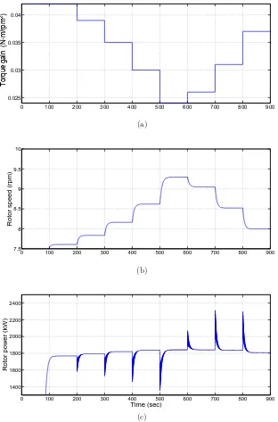
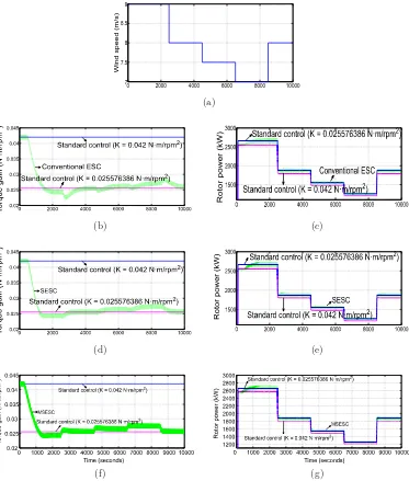
3.5 Responses of the rotor speed and rotor power under step torque gains for the NREL offshore 5-MW baseline wind turbine model. . . 34

3.6 Simulation results under a constant wind of 8 m/s along with a wave input. . . 36

(10)

3.8 Simulation results with MSESC under a step wind (see Figure 3.7a) along with a wave input. . . 37 3.9 Simulation results under step winds (without turbulence) along with

a wave input. . . 38 3.10 Simulation results under step winds (with 2% turbulence) along with

a wave input. . . 40 3.11 Simulation results under a wind input with a mean speed of 7 m/s

and 15% turbulence along with a wave input. . . 41 4.1 Schematic diagram of the TMD systems used in the John Hancock

Tower in Boston and the Citicorp Center in Manhattan [8]. . . 44 4.2 Deflections of the NREL monopile 5-MW baseline turbine tower at a

certain time instant by a FAST simulation. . . 46 4.3 Comparisons between the distributed properties of the mass density &

flexural rigidity of the NREL monopile 5-MW baseline wind turbine tower and their corresponding fitted functions ρ(x) & EI(x). The blue triangles represent distributed tower properties given in Table 2.3 while the red solid lines are their corresponding fitted functions. 57 4.4 Time simulation (in seconds) of the fore-aft tower-top translational

displacement (in meters) of the NREL monopile 5-MW baseline tur-bine tower stabilised by a fore-aft TMD under a wind input with a mean speed of 10 m/s and turbulence intensity of 15%, obtained from Σd (4.48)–(4.49) (red dotted line) and FAST (blue dash line)

respectively. . . 57 4.5 Simulation of the fore-aft translational deflections of the NREL monopile

5-MW baseline turbine tower stabilised by a fore-aft TMD under a wind input with a mean speed of 10 m/s and turbulence intensity of 15%, obtained from Σd (4.48)–(4.49) (red dotted lines) and FAST

(11)

4.6 Time simulation (in seconds) of the side-to-side tower-top transla-tional displacement (in meters) of the NREL monopile 5-MW baseline turbine tower stabilised by a side-to-side TMD under a wind input with a mean speed of 10 m/s and turbulence intensity of 15%, ob-tained from Σd (4.48)–(4.49) (red dotted line) and FAST (blue dash

line) respectively. . . 58 4.7 Simulation of the side-to-side translational deflections of the NREL

monopile 5-MW baseline turbine tower stabilised by a side-to-side TMD under a wind input with a mean speed of 10 m/s and turbulence intensity of 15%, obtained from Σd (4.48)–(4.49) (red dotted lines)

and FAST (blue dash lines) respectively. The upper, middle and lower diagrams show results at 100 s, 200 s and 300 s, respectively. The horizontal axis denotes the translational tower deflections (in meters) with positive value meaning ‘right’ and negative value meaning ‘left’, while the vertical axis describes the height of the tower (in meters). 59 4.8 Power spectral density (PSD) of tower-top fore-aft translational

dis-placement of the NREL monopile 5-MW baseline turbine tower under a wind input with a mean speed of 10 m/s and turbulence intensity of 15%, obtained from Σd (4.48)–(4.49) (red dotted and yellow

dash-dotted lines denoting cases of sole tower and tower stabilised by a fore-aft TMD, respectively) and FAST (blue solid and green dash lines denoting cases of sole tower and tower stabilised by a fore-aft TMD, respectively). . . 59 4.9 Power spectral density (PSD) of tower-top side-to-side translational

displacement of the NREL monopile 5-MW baseline turbine tower under a wind input with a mean speed of 10 m/s and turbulence in-tensity of 15%, obtained from Σd(4.48)–(4.49) (red dotted and yellow

(12)

4.10 Power spectral density (PSD) of the tower-top fore-aft translational deflections of the NREL 5-MW monopile wind turbine tower based on FAST simulations under a wind input with a mean speed of 18 m/s and turbulence intensity of 15%, and a wave input with the significant wave height of 3.5 m. Blue solid and red dotted lines denote cases of sole tower and tower stabilised by optimal fore-aft and side-to-side TMDs designed in Section 4.1.3, respectively. . . 65 4.11 Power spectral density (PSD) of the tower-top side-to-side

transla-tional deflections of the NREL 5-MW monopile wind turbine tower based on FAST simulations under a wind input with a mean speed of 18 m/s and turbulence intensity of 15%, and a wave input with the significant wave height of 3.5 m. Blue solid and red dotted lines denote cases of sole tower and tower stabilised by optimal fore-aft and side-to-side TMDs designed in Section 4.1.3, respectively. . . 65 4.12 An SCOLE beam system stabilised by multiple groups of TMDs. . . 67 4.13 Mode shapes of the first two modes of the SCOLE model. The

left-hand diagram shows the mode shape of the first mode while the right-hand one is the mode shape of the second mode. . . 76 4.14 Beam-top displacement RMS values of the SCOLE model stabilised

by TD,Ths1 andThm1 in Table 4.3 versus the excitation frequencyωe. 79

4.15 Peak beam-top displacement RMS values of the SCOLE model sta-bilised by the TMD systems in Table 4.3 versus the coefficient α for the flexural rigidity functionEI under harmonic excitations. . . 80 4.16 Beam-top displacement RMS values of the SCOLE model stabilised

byThs1 &Thm1 in Table 4.3 andTrs1 &Trm1 in Table 4.5 versus the

excitation frequencyωe. . . 81

4.17 Peak beam-top displacement RMS values of the SCOLE model sta-bilised by Ths4 & Thm4 in Table 4.3 and Trs4 & Trm4 in Table 4.5

versus the coefficient α for the flexural rigidity function EI under harmonic excitations. . . 82 4.18 PSD of beam-top displacements of the SCOLE model stabilised by

TW,Trs1 andTrm1 in Table 4.5. . . 84

(13)

4.20 Mean SDs of beam-top displacements of the SCOLE model stabilised by T_rs4 & T_rm4 in Table 4.5 and T_hs4 & T_hm4 in Table 4.3 versus the coefficientα for the flexural rigidity functionEI under random

exci-tations. . . 86

5.1 Block diagram showing the integration of the HST drivetrain model, torque and pitch controllers (together with their actuators), and FAST in the Simulink environment. . . 93

5.2 Hankel singular values of the 23rd-order plant Gm. . . 95

5.3 Bode frequency responses of the original 23rd-order plantGm and its reduced 9th-order modelGrm. . . 97

5.4 Control structure of the motor displacement controller Km. . . 97

5.5 Closed-loop step response. . . 99

5.6 Control structure of the LPV blade pitch controller Kp( ¯V). . . 101

5.7 fωr/(Jr +Jp) and fβ/(Jr +Jp) at ¯V ∈ Θ ( ¯V is the steady rotor effective wind speed). . . 101

5.8 Steady pitch angle ¯β( ¯V) ( ¯V is the steady rotor effective wind speed) [7]. . . 102

5.9 Anti-windup compensation scheme for the LPV pitch controller. . . 103

5.10 Circular pulsed LIDAR scan trajectory optimised by Schipf et al. [9] for the NREL offshore 5-MW baseline turbine model. The thick red line represents the laser beam. . . 106

5.11 Normalised Gaussian shape range weighting functionfrw(r) [9]. . . . 108

5.12 Configuration of the PI pitch controller with back-calculation AW compensation. . . 109

5.13 Actual and estimated (by LIDAR) rotor effective wind speeds (V and ¯ V) under the turbulent wind input with a mean speed of 11.4 m/s (top) or 18 m/s (bottom) along with a wave input. . . 110

5.14 Pressure commandPpdand actual pressure difference across the pump Pp under the turbulent wind input with a mean speed of 11.4 m/s (top) or 18 m/s (bottom) along with a wave input. . . 111

(14)

5.16 Simulation results under the turbulent wind input with a mean speed of 18 m/s along with a wave input. Figures 5.16a, 5.16b, 5.16c, 5.16d, and 5.16e depict the rotor speed, collective blade pitch angle, gener-ator power, and monopile base fore-aft and side-to-side moments, respectively. . . 113 5.17 Rotor speed responses under the turbulent wind input with a mean

speed of 18 m/s along with a wave input. . . 115 6.1 Barge with the BTLCD reservoir fixed on it. . . 120 6.2 Three-view drawing of the BTLCD reservoir. . . 121 6.3 Barge pitch displacement q4, tower-top displacement (TTD), and

liquid displacement qn+1/qn+3 obtained from simulations using the

transformed 5-MW barge HWT model within FAST (blue solid lines) and the simplified turbine-reservoir model Σp (6.21) (red dotted lines).128

6.4 The hub-height longitudinal wind speed and wave elevation in the extreme event for the tower-base fore-aft bending moment. . . 131 6.5 Simulations results for the transformed NREL 5-MW barge HWT

model in the cases without (blue solid lines) and with (red dash lines) the BTLCD configuration, in the extreme event for the tower-base fore-aft bending moment. Figure 6.5a, 6.5b, 6.5c and 6.5d depict the barge pitch and roll displacements, the rotor speed and the generator power,respectively. . . 134 6.6 Liquid displacements u1, u3, u5 and u7 in the four vertical columns

numbered 1, 3, 5 and 7 of the BTLCD reservoir for the transformed NREL 5-MW barge HWT model with the BTLCD configuration, in the extreme event for the tower-base fore-aft bending moment. . . . 135 6.7 The hub-height longitudinal wind speed and wave elevation in the

extreme event for the tower-base side-to-side bending moment. . . . 135 6.8 Simulations results for the transformed NREL 5-MW barge HWT

(15)

6.9 Liquid displacements u1, u3, u5 and u7 in the four vertical columns

numbered 1, 3, 5 and 7 of the BTLCD reservoir for the transformed NREL 5-MW barge HWT model with the BTLCD configuration, in the extreme event for the tower-base side-to-side bending moment. . 137 6.10 The hub-height longitudinal wind speed and wave elevation in the

normal event where the mean hub-height longitudinal wind speed is 9 m/s. . . 137 6.11 Simulations results for the transformed NREL 5-MW barge HWT

model in the normal event where the mean hub-height longitudinal wind speed is 9 m/s. Figures 6.11a, 6.11b, 6.11c and 6.11d depict the barge pitch and roll displacements, the rotor speed, and the generator power, respectively. . . 138 6.12 Liquid displacements u1, u3, u5 and u7 in the four vertical columns

numbered 1, 3, 5 and 7 of the BTLCD reservoir for the transformed NREL 5-MW barge HWT model with the BTLCD configuration, in the normal event where the mean hub-height longitudinal wind speed is 9 m/s. . . 139 6.13 The hub-height longitudinal wind speed and wave elevation in the

normal event where the mean hub-height longitudinal wind speed is 18 m/s. . . 139 6.14 Simulations results for the transformed NREL 5-MW barge HWT

model in the normal event where the mean hub-height longitudinal wind speed is 18 m/s. Figures 6.14a, 6.14b, 6.14c and 6.14d depict the barge pitch and roll displacements, the rotor speed, and the generator power, respectively. . . 140 6.15 Liquid displacements u1, u3, u5 and u7 in the four vertical columns

(16)

Acknowledgments

(17)

Declarations

This thesis is submitted to the University of Warwick in support of my application for the degree of Doctor of Philosophy. It has been composed by myself and has not been submitted in any previous application for any degree.

Parts of this thesis have been published by the author:

Journal (Peer Reviewed)

a. X. Tong and X. Zhao, “Power generation control of a monopile hydrostatic wind turbine using an _H∞ loop-shaping torque controller and an LPV pitch controller,” IEEE Transactions on Control Systems Technology, 2017, DOI: 10.1109/TCST.2017.2749562.

b. X. Tong, X. Zhao, and S. Zhao, “Load reduction of a monopile wind turbine tower using optimal tuned mass dampers,” International Journal of Control, vol. 90, no. 7, pp. 1283–1298, 2017.

c. X. Tong, X. Zhao, and A. Karcanias, “Passive vibration control of an offshore floating hydrostatic wind turbine,” Wind Energy, accepted subject to revision. d. X. Tong and X. Zhao, “Passive vibration control of the SCOLE beam system,”

Structural Control and Health Monitoring, accepted subject to revision.

Conference (Peer Reviewed)

a. X. Tong and X. Zhao, “LPV pitch control of a hydrostatic wind turbine based on LIDAR preview,” in2017 American Control Conference, WA, USA, May 2017. b. X. Tong and X. Zhao, “Vibration suppression of the finite-dimensional approxi-mation of the non-uniform SCOLE model using multiple tuned mass dampers,” in55th IEEE Conference on Decision and Control, NV, USA, December 2016. c. X. Tong, X. Zhao, and S. Zhao, “Passive structural vibration control of a

monopile wind turbine tower,” in 54th IEEE Conference on Decision and Con-trol, Osaka, Japan, December 2015.

(18)

Abstract

Several control strategies are proposed to improve overall performances of conven-tional (geared equipped) and hydrostatic offshore wind turbines.

Firstly, to maximise energy capture of a conventional turbine, an adaptive torque control technique is proposed through simplifying the conventional extremum seeking control algorithm. Simulations are conducted on the popular National Re-newable Energy Laboratory (NREL) monopile 5-MW baseline turbine. The results demonstrate that the simplified ESC algorithms are quite effective in maximising power generation.

Secondly, a TMD (tuned mass damper) system is configured to mitigate loads on a monopile turbine tower whose vibrations are typically dominated by its first mode. TMD parameters are obtained viaH2 optimisation based on a spatially

discretised tower-TMD model. The optimal TMDs are assessed through simulations using the NREL monopile 5-MW baseline model and achieve substantial tower load reductions. In some cases it is necessary to damp tower vibrations induced by multiple modes and it is well-known that a single TMD is lack of robustness. Thus a control strategy is developed to suppress wind turbine’s vibrations (due to multiple modes) using multiple groups of TMDs. The simulation studies demonstrate the superiority of the proposed methods over traditional ones.

(19)

(20)

Abbreviations

ADAMS Automatic Dynamic Analysis of Mechanical Systems

AW anti-windup

BTLCD bidirectional tuned liquid column damper

CAE computer-aided-engineering

COM centre of mass

CW continuous wave

DD Digital Displacement

DEQL damage equivalent load

DFIG doubly fed induction generator

DLL dynamic-link-library

DOF degree of freedom

EOM equation of motion

ESC extremum seeking control

ETM extreme turbulence model

EWEA European Wind Energy Association

FAST Fatigue, Aerodynamics, Structures, and Turbulence

FEM finite element method

FRC fully rated converter

HAWT horizontal-axis wind turbine

HPF high-pass filter

HSS high-speed shaft

HST hydrostatic transmission

(21)

IEC International Electrotechnical Commission

IMU inertial measurement unit

LDA Laser Doppler Anemometry

LDV Laser Doppler Velocimetry

LIDAR Light Detection and Ranging

LOS line-of-sight

LPF low-pass filter

LPV linear parameter varying

LSS low-speed shaft

MHI Mitsubishi Heavy Industries

MSESC more simplified extremum seeking control

MSL mean sea level

NREL National Renewable Energy Laboratory

NTM normal turbulence model

NWP normal wind profile

O&M operation & maintenance

OC3 Offshore Code Comparison Collaboration

PDE partial differential equation

PIV Particle Imaging Velocimetry

PMG permanent magnet generator

PRC partial rated converter

PSD power spectral density

RMS root-mean-square

RNA rotor nacelle assembly

SCOLE Spacecraft Control Laboratory Experiment

SD standard deviation

SESC simplified extremum seeking control

SH sample-and-hold

SODAR SOnic Detection And Ranging

(22)

TLCD tuned liquid column damper

TLCSD tuned liquid column and sloshing damper

TLSD tuned liquid sloshing damper

TMD tuned mass damper

TSR tip-speed ratio

TTD tower-top displacement

ULF ultimate load factor

VAWT vertical-axis wind turbine

(23)

Chapter 1 Introduction

1.1 Wind Energy

Wind power has been used as a clean source of renewable energy with sustainable growth in penetration and investments. By 2015, the global installed wind power capacity had reached 432.9 GW [10], surging from only 74 GW in 2006 [11]. The United States aims to install 100,000 MW of wind power by 2020 [3]. By the same year, the EU is estimated to install 230 GW of capacity which will meet 15–17% of EU electricity demand. This will save Europe about ¤_{8.5 billion of CO}₂ _{cost per} year [12]. Electricity generated from wind is predicted to make up 9.1% of world electricity generation in 2020 [13].

(24)

installed offshore wind capacity is expected to reach 75 GW [18].

The motivations for the significantly increasing offshore wind installation are as follows:

a. The global offshore wind resource is abundant. For instance, the UK’s total available offshore wind capacity is estimated to be 675 GW which is more than 6 times the present UK electricity demand [19].

b. The wind tends to blow faster offshore than on land. A small increase in wind speed induces a considerable growth in energy generation, e.g., a turbine in a 15-mph wind can produce twice as much electricity as it does in a 12-mph wind [20]. Hence, much more energy can be generated offshore.

c. Offshore wind is less turbulent than on land and thus is a more reliable energy source.

d. Offshore wind farms cause no noise effect or visual impact if located sufficiently off the coast.

e. The huge area of offshore zones enables turbine installations without hindering other land utilisations [4].

1.2 Wind Turbine System

Wind turbines are designed to convert the kinetic energy of local wind into electric-ity. They can rotate about either a horizontal axis or a vertical axis, the former and the latter being named horizontal-axis wind turbines (HAWTs) and vertical-axis wind turbines (VAWTs) respectively. Since HAWTs are able to produce more elec-tricity from a given amount of wind than VAWTs, they dominate the wind industry. Figure 1.1 shows the tower and RNA (rotor nacelle assembly) of a modern typical conventional HAWT. The RNA is located at the top of the tower. The rotor com-prises the blades and hub. The nacelle supports the generator and drivetrain. The drivetrain of a conventional HAWT is a series of mechanical components including the low-speed shaft (LSS), the gearbox, and the high-speed shaft (HSS). When wind blows past the blades, it lifts and rotates them, causing the rotor shaft to spin, thus capturing wind energy. This process triggers the LSS connected to the gearbox to spin. The gearbox increases the LSS speed into the HSS speed. The HSS drives the generator to produce electricity. In Figure 1.1, the rotor is in upwind position (facing the wind) and has three blades. This design is generally adopted by HAWT rotors mainly due to the following factors:

a. An upwind design avoids the wind shade behind the tower.

(25)

[image:25.595.201.439.107.350.2]

Figure 1.1: Tower and RNA of a modern typical conventional HAWT. This figure is taken from the paper [3].

in wind speed with altitude), yawing, etc. For three-bladed turbines, these cyclic loads are symmetrically balanced when combined together at the LSS, produc-ing a constant load at the drivetrain. However, for one- and two-bladed wind turbines, they combine into a fluctuating load which leads to unnecessary wear on the drivetrain. Hence, one- and two-bladed wind turbines require teetering hubs to reduce this load, which adds complexity to the turbine design.

c. More than three blades are rarely used primarily because of the higher costs associated with the additional blades.

(26)

Figure 1.2: Monopile (left) and barge (right) substructures of offshore wind turbines [4].

be the most economical [21]. The National Renewable Energy Laboratory (NREL) has proposed a floating substructure concept—a barge with barge-fastened mooring lines anchored to the seabed to hold the barge in position against winds and waves (see the right-hand diagram in Figure 1.2). This substructure is simple in its design, fabrication, and installation [4].

(27)

1.3 Hydrostatic Wind Turbine

The gearbox of a conventional offshore turbine (see Figure 1.1) is one of the largest contributors to the turbine’s overall operation & maintenance (O&M) cost [24, 25] due to several reasons:

a. Gearboxes suffer high failure rates principally resulting from underestimation of actual operating loads, impact loads on bearings (under unexpected operat-ing conditions, e.g., grid loss, grid faults, wind gusts, etc.), and misalignment between the gearbox output shaft and the HSS [26]. Their failure rates grow as turbines are built offshore with increasingly large sizes. This is mainly due to three reasons. First, turbines with larger sizes tend to fail more frequently [27, 28]. Second, gearbox bearings have to bear higher loads caused by higher wind speeds and harsher weather offshore. Finally, it is difficult to access offshore turbines, and unfavourable offshore weather conditions hamper maintenance ser-vices. According to the paper [25] which investigated about 350 European off-shore turbines (2–4 MW) over 5 years, the gearbox is the largest contributor making up 59% of the turbine failures which require major component replace-ments.

b. The gearbox repair cost is high predominantly because of expensive crane ser-vices required. The paper [25] showed that the average replacement cost of the gearbox is¤_230,000.

c. The gearbox also causes the longest downtime per failure among all the turbine components [29]. One reason is that its complex repair procedures incur high repair time per failure. The average repair time for a major gearbox replacement can be as long as 10 days [25]. Travel time and probably delayed maintenance due to unfavourable offshore weather also contribute to the long downtime. As calculated by Ran et al. [30], the daily average revenue loss during the downtime of a 4-MW offshore turbine is as high as£_6,720.

d. The gearbox is one of the components requiring the most technicians after failing, resulting in high labour costs per failure. The paper [25] recorded an average of 17.2 technicians needed for a major gearbox replacement.

(28)

Figure 1.3: Main components of a typical HST drivetrain in the HWT and their connections [5].

that of its geared equipped counterpart [31]. However, direct-drive PMGs still have the following downsides:

a. The manufacturing cost of a PMG is nearly 40% higher than that of a doubly fed induction generator (DFIG, normally used in a geared equipped turbine) with the same rated power [32].

(29)

lowers the turbine capital cost and reduces power losses (due to the inefficiency in the switching operation of power electronics) [35].

The motor & generator of an HST drivetrain can be either configured at the tower base or in the nacelle. The tower-base HST configuration can reduce the nacelle mass of a conventional 5-MW turbine by about 2/3 [36], which saves the costs in the supporting structures and transportation & installation of turbine components, thus reduces the turbine capital cost. The report [24] demonstrated that the O&M cost of a conventional 5-MW offshore turbine can reduce by over 60% when using the tower-base HST drivetrain based on the following facts:

a. The mean time between repairs of the HST can be more than 50% longer than the gearbox.

b. The pump/motor is composed of modular lightweight components which, when configured in the nacelle, can be repaired/replaced using the turbine’s internal hoist without the need for a costly external crane.

c. The tower-base HST configuration enables easier access to the motor and gen-erator.

d. The HWT does not need power electronics that is one of the turbine components which are most likely to fail.

According to [24], the in-nacelle HST configuration has even less O&M cost than its tower-base counterpart mainly because it has significantly shorter hydraulic lines filled with much less fluid and thus lower cost in regular fluid replacements. But the in-nacelle configuration has a higher capital cost than its tower-base counterpart because of the substantial reduction of the nacelle mass in the tower-base configu-ration. Having said that, the overall costs (including capital cost and O&M cost) are similar between the two HST configurations [24].

(30)

offshore turbine.

1.4 Wind Turbine Control

Both a conventional turbine and an HWT have 2 control levels [3]. The upper level is accomplished by a supervisory controller which starts and stops the turbine depend-ing on the detected turbine and wind conditions. On the lower level is closed-loop control including torque control, blade pitch control, yaw control, and structural control. The torque controller regulates the rotor reaction torque and thus the rotor speed, through controlling the generator torque for a conventional turbine or the displacement of the hydraulic machine for an HWT. The blade pitch controller gen-erates the blade pitch command following which the pitch actuator turns the blade to keep the rotor speed within its operating limits as the wind speed varies. The yaw control system (including the brake, the yaw drive, and the yaw motor as shown in Figure 1.1) rotates the rotor to face into the wind, ensuring maximal electric power to be extracted as the wind direction changes. Since yaw control is slow, it interests control engineers less than torque and pitch control [3]. Structural control [39] is initially used in civil engineering to protect structures from dynamic loadings due to earthquakes, strong winds, waves, etc. It has been employed to suppress vibrations in wind turbines [40, 41, 42, 43, 44, 45]. Structural control is divided into three major categories: passive, semi-active and active control [46]. Passive structural control is the simplest among them since it needs no external power and uses structural motions to generate control forces. A semi-active structural control device requires power from a small external source and uses structural motions to develop control forces which are regulated by the power source. An active structural control system requires a large power source to produce control forces based on the measurements of external excitations and/or structural responses [47]. In this the-sis, only closed-loop control (more specifically, torque, pitch, and passive structural control) is considered.

(31)

Figure 1.4: Steady-state power-versus-wind-speed curve of turbines.

power coefficientCp defined as the ratio of the rotor powerprto the available power

from the wind pwind:

Cp= pr

pwind

(1.1) where

pr=τaeroωr, pwind=

1 2ρaπR

2_V3_. _(1.2)

τaerois the aerodynamic torque extracted by the rotor from the wind,ωris the rotor

shaft speed,ρa is the air density,R is the rotor radius, and V is the rotor effective

wind speed. The tip-speed ratio (TSR) is

λ= ωrR

V . (1.3)

Cpis a function ofλand the blade pitch angleβ, and it has a unique global maximum

C_p∗ at λ = λ∗ and β = β∗ (the superscript star denotes an optimal value) [3]. In Region 2, the blade pitch controller does not work and saturates the pitch angle at its lower limit which is set to beβ∗. Thus, maximising wind power extraction means maintaining Cp at its maximum Cp∗ through regulating the rotor speed to

(32)

1.5 Motivations and Research Contributions

The focus of this thesis is performance improvements of both conventional (geared equipped) and hydrostatic offshore wind turbines in the following aspects:

a. According to the paper [3], if the US achieves its goal of 100,000 MW of wind power installation by 2020, a 3% loss in wind energy capture would cause a loss of

$_{300 million per year. Hence, the development of a torque controller to effectively}

maximise the power capture in Region 2 is of great necessity. An adaptive torque control technique is proposed through simplifying the conventional extremum seeking control (ESC) algorithm. The simulations on the popular NREL 5-MW baseline monopile turbine model show that the proposed method enhances the turbine’s energy capture over a standard control law.

b. As offshore turbines are getting larger and deployed further offshore, towers are required to be stronger and heavier in order to support heavier tower-top masses, and stand against more severe weather, turbulence, and wave conditions. This incurs expensive structural supporting materials and high transportation & installation costs for turbine components. A feasible solution to this issue is to develop control techniques to mitigate vibration loads acting on turbine towers, which enables the construction of lighter and cheaper towers, and increases the towers’ life expectancy. The load reduction of a monopile-tower assembly (also referred to as a monopile tower) is investigated. Because the first tower bending mode dominates the dynamic response of a typical monopile tower [48], tower loads can be significantly reduced by only damping vibrations caused by the first tower mode. For this purpose a tuned mass damper (TMD) system is configured on the nacelle floor. The monopile turbine is modelled using a non-uniform NASA SCOLE (Spacecraft Control Laboratory Experiment) system. Based on it tower dynamics can be accurately simulated, and optimal TMD parameters can be derived through_H2 optimisation. The optimal TMD system

is validated to considerably mitigate the tower loads through simulations using the NREL 5-MW baseline monopile turbine model (see also [49, 50]). This work also demonstrates how to optimally tune a TMD to reduce vibrations of a flexible structure described by partial differential equations (PDEs).

(33)

the original first tower mode (because the first tower modal frequency deviates from its original value used for the TMD design), but also possibly cause in-creased coupling between higher tower modal frequencies and rotor harmonic frequencies. The latter phenomenon was observed by [54] where the second tower bending modal frequency coincided with the 6P (with 1P being the rotor rotational frequency) rotor harmonic frequency (resulting in higher loads and larger fatigue damage to the monopile tower). Therefore, it is worth developing a control scheme to suppress multiple tower vibration modes simultaneously and at the same time improve robustness of the TMD system. Accordingly, the pre-ceding TMD optimisation scheme is extended to the design of multiple TMDs for the vibration reduction of the non-uniform SCOLE beam system (used above to model monopile turbine towers) with multiple dominant vibration modes. Note that the SCOLE model rather than the NREL monopile tower is used as the illustrative application, because the former can be parameterised to have multiple dominant modes while the latter has only one dominant mode. The extended control method takes into account the trade-off between effectiveness and robustness when optimising multiple TMDs. Through simulation studies, the optimal multiple TMDs are shown to be quite effective in damping multi-ple vibration modes simultaneously and are robust against variations of modal frequencies of the SCOLE model (see also [55, 56]).

(34)

very good tracking behaviour while the LPV pitch controller (no matter with or without AW) gets much improved overall performances over a gain-scheduled PI pitch controller (see also [57, 58]).

e. The barge (see Figure 1.2) is a quite promising substructure for a floating tur-bine. However, its rotational motions can not only cause large fluctuations in the rotor speed and generator power, but also cause considerable load varia-tions on the turbine, especially on the tower base [4]. For a barge HWT with a tower-base HST configuration where the reservoir can be placed on the barge, a spin-off application of the reservoir is proposed to suppress pitch and roll motions of the barge. More specifically, the reservoir is made into a shape of an annular rectangular to serve as a bidirectional tuned liquid column damper (BTLCD). This means a barge-motion damper is configured with negligible extra costs as an HST needs a reservoir anyway. The coupled dynamics of the barge-reservoir system are incorporated into the transformed HWT model (mentioned above) with the NREL barge substructure by using Lagrange’s equations. Two simpli-fied turbine-reservoir models are used to optimise the parameters of the BTLCD reservoir, which describe the pitch and roll motions of the turbine-reservoir sys-tem respectively. Simulation results based on the barge HWT model show that the optimal BTLCD reservoir is very effective in mitigating pitch and roll mo-tions of the barge under realistic wind and wave excitamo-tions, which reduces the tower load and improves the power quality (see also [59, 60]).

1.6 Thesis Outline

This thesis is organised as follows. Chapter 2 introduces several NREL computer-aided-engineering (CAE) tools (TurbSim, FAST, and MLife) and the NREL offshore 5-MW baseline (geared equipped) wind turbine model. Chapter 3 investigates max-imum power capture of a conventional wind turbine operating in Region 2 using the conventional ESC algorithm and its two simplified versions. Chapter 4 first studies the load reduction of a monopile wind turbine tower using a TMD system derived throughH2optimisation. Then it extends this research to suppress vibrations of the

(35)

(36)

Chapter 2 NREL Computer-Aided

Engineering Tools and NREL

Offshore 5-MW Baseline Wind

Turbine Model

This chapter introduces NREL computer-aided-engineering (CAE) tools TurbSim, FAST, and MLife, as well as the NREL offshore 5-MW baseline (geared equipped) wind turbine model. In this thesis, they are used for the design of controllers and simulation studies.

2.1 Stochastic Inflow Turbulence Simulator—TurbSim

NREL TurbSim is utilised to simulate stochastic, full-field, and turbulent wind flows. TurbSim generates a time series of wind speed vectors at points in a two-dimensional vertical rectangular grid fixed in space [61]. Each wind speed vector has three components: u (longitudinal—along the direction of the mean wind velocity), v (crosswise—perpendicular to u and horizontal), and w (vertical—perpendicular to u and v). The height and width of the grid, and the numbers of vertical and crosswise grid points can be specified in the TurbSim input file. The grid points are uniformly distributed in both the crosswise and vertical directions. The grid top is aligned with the rotor disk top, and the grid bottom must be above the mean sea level (MSL). The rotor is crosswise centred on the grid.

(37)

wind speeds at the grid points with the same height. The IEC Kaimal spectral model (giving a good description of atmospheric turbulence [62]) with either the IEC normal turbulence model (NTM) or the IEC extreme turbulence model (ETM) is utilised to determine wind data. The data contain spectra of the three wind com-ponents and the spatial coherence between wind speed vectors at any two different grid points in the frequency domain. With these data, TurbSim uses an inverse Fourier transform to create the time series.

2.1.1 Normal Wind Profile Model

The IEC NWP model gives the mean value ofu-component wind speeds at the gird points with the same heightzas

¯

u(z) = ¯uhub

z zhub

αpl

(2.1)

where ¯uhub is the meanu-component wind speed at the hub height,zhub is the hub

height, and αpl is the power law exponent whose default value is 0.14 for offshore

wind turbines [62]. The meanv−and w−component wind speeds are zero at all the grid points.

2.1.2 IEC Kaimal Spectral Model with NTM/ETM

The IEC Kaimal spectral model describes the relationships among standard devi-ations of the three wind components (σK where K = u, v, w) at each grid point

as

σv = 0.8σu, σw = 0.5σu. (2.2)

Then the spectra of the three wind components at each grid point are

SK(f) =

4σ_K2 LK/¯uhub

1 + 6f LK/¯uhub

5/3 (2.3)

wheref is the frequency in Hz. LK is the integral scale parameter:

LK =

          

8.10Λu, K =u

2.70Λu, K =v

0.66Λu, K =w

(38)

Λu is the turbulence scale parameter:

Λu= 0.7 min (60m, zhub). (2.5)

If using the standard IEC turbulence category A, B, or C (with A being the most turbulent) to specify the turbulence intensityIturb, the IEC NTM determines

σu as below to derive (2.2) and (2.3):

σu =Iturb(0.75¯uhub+ 5.6) (2.6)

where

Iturb =

          

0.16, category A 0.14, category B 0.12, category C

. (2.7)

If specifyingIturb in percent, the IEC NTM determines σu as

σu =

Iturb

100u¯hub. (2.8) The IEC ETM only acceptsIturb specified using the standard IEC turbulence

cate-gory. The IEC ETM has three classes: 1, 2, and 3. It calculates σu as

σu = 2Iturb 0.072 0.1Vref + 3

¯ uhub

2 −4

+ 10 !

. (2.9)

Vref is the reference wind speed:

Vref =

          

50 m/s, Class 1 42.5 m/s, Class 2 37.5 m/s, Class 3

. (2.10)

The IEC Kaimal model defines the spatial coherence between theu-components at grid pointsi andj as

Cohi,j(f) =exp

 −12

(39)

wherer is the distance between pointsiand j. Lc is the coherence scale parameter:

Lc = 5.67 min(60m, zhub). (2.12)

The spatial coherence between thev−/w−components at pointsiand j is

Cohi,j(f) =

    

1, i=j 0, i₆=j

. (2.13)

2.2 Simulator of Wind Turbine Dynamics—FAST

The NREL FAST code is widely employed for simulating aerodynamics, hydrody-namics, control and electrical (servo) dyhydrody-namics, and structural (elastic) dynamics of offshore turbines. In FAST, equations of motion are set up using Kane’s method and solved by numerical integrations [4]. Before running FAST, properties of a turbine composed of rigid and flexible bodies must be specified in its input files to construct a wind turbine model. The rigid bodies include the earth, nacelle, hub, and substructure of a floating turbine while the flexible bodies include the tower, blades, drive shaft, and substructure of a fixed-bottom turbine. These bodies are coupled using several degrees of freedom (DOFs) including the tower bending, blade bending, rotor speed, and drive shaft torsional DOFs. FAST has 6 DOFs for the floating rigid substructure: translational surge, sway, & heave DOFs, and rotational roll, pitch, & yaw DOFs. All the DOFs can be switched on or off in FAST input files.

FAST utilises several coordinate systems for input and output parameters. Its inertial coordinate system I has the origin O and the set of orthogonal axes

xI,yI,zI. Ois the substructure reference point. The 6 floating substructure motion DOFs are defined about it on which the external loads act [4]. ThexI-axis points in the nominal downwind direction, the xIyI-plane designates the mean sea level (MSL), and the zI-axis points upward opposite to gravity along the undeflected tower’s centreline when the substructure is undisplaced. FAST has a nacelle inertial measurement unit (IMU) whose location is user-prescribed. FAST can output the displacement, velocity, and acceleration of the nacelle IMU relative to _I. u, v, w components of the wind speed vector generated by TurbSim are defined in_I [61]. The nacelle coordinate system in FAST is denoted asN which is fixed on the tower top and moves with the nacelle. It has the originOs (the intersection of the tower’s

(40)

[image:40.595.162.479.340.560.2]

Figure 2.1: Schematic of FAST modules for a fixed-bottom turbine [6].

Figure 2.2: Schematic of FAST modules for a floating turbine [6].

(41)

Figure 2.3: Configuration of the in-nacelle TMD system in ServoDyn.

at these nodes through interpolating the time series from TurbSim in time and space based on Taylor’s frozen turbulence hypothesis (assuming that the turbulent wind field moves with the mean hub-height wind speed ¯uhub), and outputs them

(42)

two-dimensional slices and calculates hydrodynamic loads by integrating the loads acting on each slice over the substructure length. Strip-theory hydrodynamic loads include added mass and incident-wave inertia loads, and viscous drag associated with the relative velocity between the seawater and the substructure [4]. For the NREL barge, the combination of strip and flow theories is used. The potential-flow theory provides hydrodynamic loads including excitation loads from incident waves, hydrostatic restoring loads, and added mass & damping loads associated with wave radiation. The strip theory produces viscous drag. The potential-flow method necessitates hydrodynamic coefficients which must be supplied by a separate numerical-panel code, e.g., WAMIT (Wave Analysis at MIT) used by FAST [64]. HydroDyn incorporates several incident wave kinematics model to describe wave elevations (closely related to wave-excitation loads). The JONSWAP spectrum is chosen to model irregular waves with no currents. This model depends on two user-prescribed parameters—the significant wave height and peak-spectral period of waves [4].

FAST can be interfaced with MATLAB/Simulink through a Simulink S-Function block. During simulations, this block calls the FAST Dynamic Library which is compiled as a dynamic-link-library (DLL) integrating all the FAST mod-ules [65]. This enables flexible turbine modelling and control design in the Simulink environment. Besides, FAST can conduct linearisation analyses. Before linearisa-tion, an operating point is specified as a set of steady values of the enabled DOF displacements, velocities, & accelerations, and control & wind inputs. FAST nu-merically linearises the non-linear turbine model at this point by perturbing system variables about their respective steady values, which results in a linear state-space model. In addition, FAST can work as an ADAMS (Automatic Dynamic Analy-sis of Mechanical Systems) preprocessor. It can generate an ADAMS dataset of a complete aero-hydro-servo-elastic wind turbine model [65] which can be input to the ADAMS Aggregate Mass tool to derive the values of some useful turbine parameters [66].

2.3 Estimator of Fatigue Life—MLife

NREL MLife is employed to compute the short-term damage equivalent load (DEQL) which is usually regarded as a measurement of the fatigue load. MLife break downs the load time series from the FAST simulation into a set of cycles, and computes the load mean and load range of each cycle, using rainflow counting [67, 68]. Then it transforms the ith cycle’s load range LR

(43)

LRF

i with a load mean LM F:

LRF_i =LR_i   

Lult− L

M F Lult₋

LM_i

 

. (2.14)

LM F is the mean of the load time series and is the same for all the cycles. Lult represents the ultimate design load obtained by multiplying the maximum of the time series with an ultimate load factor (ULF) which is set to be 20 according to the report [69]. Then MLife bins each cycle. The number of load-range bins is set to be 60 following Sutherland [70]. The width of each bin is

∆R= L

R max

60 (2.15)

whereLR_max is the maximumLRF_i . The bin indexk for the load rangeLRF_i is

k=     LRF i ∆R !    (2.16)

where_⌈x_⌉ is the smallest integer not less than x. Then the load-range valueLR

k for

thekth bin is

LR_k =

k−1

2

∆R. (2.17)

The short-term DEQL DEQLST F is defined as a constant-amplitude load applied over the elapsed time of the time series Tet which produces the same damage as

caused by the loads from the FAST simulation overTet[67]:

DEQLST F =      P k

nF_k LR_km feq_T

et      1 m (2.18)

wherenF

k is the total number of cycles whose transformed load rangesLRFi fall into

(44)

[image:44.595.138.508.144.513.2]

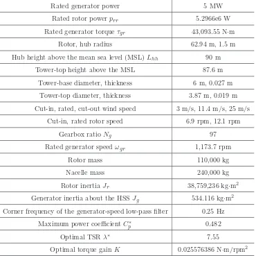
Table 2.1: Selected gross properties of the NREL offshore 5-MW baseline wind turbine model.

Rated generator power 5 MW

Rated rotor powerprr 5.2966e6 W

Rated generator torqueτgr 43,093.55 N·m

Rotor, hub radius 62.94 m, 1.5 m

Hub height above the mean sea level (MSL)Lhh 90 m

Tower-top height above the MSL 87.6 m

Tower-base diameter, thickness 6 m, 0.027 m

Tower-top diameter, thickness 3.87 m, 0.019 m

Cut-in, rated, cut-out wind speed 3 m/s, 11.4 m/s, 25 m/s

Cut-in, rated rotor speed 6.9 rpm, 12.1 rpm

Gearbox ratioNg 97

Rated generator speedωgr 1,173.7 rpm

Rotor mass 110,000 kg

Nacelle mass 240,000 kg

Rotor inertiaJr 38,759,236 kg·m2

Generator inertia about the HSS Jg 534.116 kg·m

2

Corner frequency of the generator-speed low-pass filter 0.25 Hz

Maximum power coefficientC∗

p 0.482

Optimal TSRλ∗ _7.55

Optimal torque gainK 0.025576386 N_·m/rpm2

2.4 NREL Offshore 5-MW Baseline Wind Turbine Model

The well-known NREL offshore 5-MW baseline (geared equipped) wind turbine is a representative utility-scale large offshore turbine model whose dynamic responses can be simulated by FAST (see Section 2.2). Table 2.1 lists some gross properties of this turbine model [4]. The diameter and thickness of the steel tower linearly decrease from the tower base to top.

(45)

[image:45.595.122.521.265.529.2]

Table 2.2: Undistributed properties of the NREL OC3 monopile 5-MW wind turbine tower.

Monopile diameter, thickness 6 m, 0.06 m

Tower-base height above the MSL 10 m

Water depth (from the MSL down to the mudline) 20 m

Overall mass 522,617 kg

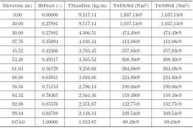
Table 2.3: Distributed properties of the NREL OC3 monopile 5-MW wind turbine tower [1].

Elevation (m) HtFract (-) TMassDen (kg/m) TwFAStif (Nm2

) TwSSStif (Nm2

)

0.00 0.00000 9,517.14 1,037.13e9 1,037.13e9

30.00 0.27881 9,517.14 1,037.13e9 1,037.13e9

30.00 0.27882 4,306.51 474.49e9 474.49e9

37.76 0.35094 4,030.44 413.08e9 413.08e9

45.52 0.42306 3,763.45 357.83e9 357.83e9

53.28 0.49517 3,505.52 308.30e9 308.30e9

61.04 0.56729 3,256.66 264.08e9 264.08e9

68.80 0.63941 3,016.86 224.80e9 224.80e9

76.56 0.71153 2,786.13 190.06e9 190.06e9

84.32 0.78365 2,564.46 159.49e9 159.49e9

92.08 0.85576 2,351.87 132.77e9 132.77e9

99.84 0.92788 2,148.34 109.54e9 109.54e9

107.60 1.00000 1,953.87 89.49e9 89.49e9

the mudline (0) to the tower top (1) along the tower centreline, TMassDen is the tower section mass per unit length, TwFAStif is the tower section fore-aft stiffness, and TwSSStif is the tower section side-to-side stiffness. The NREL ITI Energy barge is rigid, square, and moored by 8 catenary lines as illustrated in Figure 2.4 [4]. Each corner of the barge is linked to 2 lines which are 45◦ apart at the corner when the barge is undisplaced. Table 2.4 lists some tower and barge properties of the NREL ITI Energy barge 5-MW turbine model [4].

(46)

[image:46.595.200.442.106.353.2]

Figure 2.4: NREL ITI Energy barge 5-MW wind turbine [4].

Table 2.4: Selected tower and barge properties of the NREL ITI Energy barge 5-MW wind turbine model.

Barge size (width_×length_×height) 40 m_×40 m_×10 m

Tower-base height above the MSL 0 m

Water (anchor) depth (from the MSL down to the mudline) 150 m

Distance from the mass centre of

the undeflected tower & RNA toO(Lt)

63.97 m

Distance from the mass centre of the barge toO (Lp) 0.28 m

Barge massmp 5,452,000 kg

Tower mass 347,460 kg

Barge pitch inertia aboutO (Ibp) 7.27e8 kg·m2

(47)

Figure 2.5: Torque-versus-speed curve of the NREL offshore 5-MW baseline model [7].

is zero, and the turbine extracts no power from the wind. Region 1.5 is a linear transition between Regions 1 and 2 where the filtered generator speed is between 670 rpm and 871 rpm (30% above 670 rpm). As the filtered generator speed increases to above 871 rpm but below 1,161.96 rpm (99% of the rated speed of 1,173.7 rpm), the turbine works in Region 2 where the control aim is to maximise power capture. A so-called standard control law is applied to set the generator torque τg to be

proportional to the square of the filtered generator speedωf g:

τg =Kωf g2 (2.19)

where the value of the gain K (see Table 2.1) is obtained from

K = 1 2ρaπR

5 C

∗

p

(λ∗₎3_N3

g

. (2.20)

Assuming there is no torsional motion between the rotor and generator, the rota-tional motion of the rotor shaft is then described by

˙

ωr = 1

Jr+Ng2Jg

τaero−Ngτg. (2.21)

From (1.1) and (1.2), one can derive

τaero=

1 2

ρaπR2V3Cp

ωr

(48)

Combining (2.19), (2.20), (2.21), & (2.22), and assuming thatωf g =Ngωr

(neglect-ing the high-frequency noise of the rotor speed), one can derive

˙ ωr =

ρπR5ω2_r

2Jr+Ng2Jg

"

Cp

λ3 −

C_p∗

(λ∗₎3 #

. (2.23)

Clearly, if Cp <

C_p∗/(λ∗)3λ3, then ˙ωr < 0, and vice versa. It means that the

standard control law given by (2.19) and (2.20) drives λ towards the optimum λ∗ whenever the rotor speed ωr is too slow or too fast [71]. Region 2.5 is a linear

transition between Regions 2 and 3. This region is required to limit the blade tip speed around the rated power and therefore to reduce noise. Below the rated generator speed (1,173.7 rpm), the blade pitch controller does not work and saturates the pitch angle at its lower limit of 0◦. In Region 3 above the rated generator speed, the control goal is to maintain the turbine output power and generator speed around their respective rated values. Accordingly, the generator torque is set to be inversely proportional to the filtered generator speed:

τg =

prr

ωf g

. (2.24)

Note that whenever the blade pitch angle is 1◦ _{or greater, the generator torque is} calculated following (2.24) to reduce power dips and thus improve output power quality. This may incur short-term drivetrain overloads which can be avoided by setting the maximum allowable torque to be 47,402.91 N_·m (10% above the rated value of 43,093.55 N_·m). The torque rate is also limited within _±15,000 N_·m/s. A gain-scheduled proportional-integral (PI) blade pitch control on the error between ωf g and ωgr is implemented, with the gains of proportional and integral terms KP

andKI scheduled by the pitch angleβ:

KP(β) =−

2Jr+Ng2Jg

ωrrζpfp

Ng

h

∂Pr

∂β (β = 0◦)

i

1 +_βKβ

, KI(β) =−

Jr+Ng2Jg

ωrrfp2

Ng

h

∂Pr

∂β (β = 0◦)

i

1 + _βKβ ,

(2.25) whereωrr = 12.1 rpm is the rated rotor speed,∂pr/∂β(β = 0◦) =-25.52e6 W/rad is

the sensitivity of the rotor power to the pitch angle at β= 0◦, andβK = 6.302336◦

is the pitch angle at which∂pr/∂β doubles its value at β = 0◦ [7]. This scheduling

implies that the idealised response of the generator speed error will be like that of a second-order system with the natural frequency of fp and damping ratio of ζp.

(49)

recommended by the report [7], while they are advised to be 0.4 rad/s and 0.7 for the NREL ITI Energy barge 5-MW turbine [4]. The blade pitch rate is restricted within ±8◦/s. The upper limit of the blade pitch angle is 90◦.

2.5 Conclusions

Several NREL CAE tools which are used for the control design and simulation stud-ies in the following chapters are introduced. TurbSim is used to generate wind speed time series which are passed to FAST for simulating time-domain dynamics of wind turbines. FAST modules integrate aerodynamics models, hydrodynamics models, control and servo dynamics models, and structural dynamics models. FAST can be interfaced with MATLAB/Simulink, which enables simulations, turbine modelling and control design in the Simulink environment. Besides, FAST can provide lineari-sation analyses and work as the ADAMS preprocessor. To quantify fatigue loads, MLife is used to calculate short-term DEQLs through processing load time series from FAST simulations.

(50)

Chapter 3 Maximising Wind Power

Capture and Generation Based

on Extremum Seeking Control

This chapter investigates the maximum power capture for a conventional (geared equipped) wind turbine operating in Region 2 using extremum seeking control (ESC). Via ESC, the optimal torque gain is obtained with the rotor power as the optimisation objective. The conventional ESC algorithm can be simplified by omit-ting the low-pass filter (LPF) in the ESC loop and adding a sample-and-hold (SH) block. One advantage of this simplified ESC (SESC) method is that the implemen-tation of the SH is easier than the LPF because the selection of the LPF corner frequency needs not be considered. SESC also removes the influence of the LPF on the dynamics of the control system. Furthermore, even the high-pass filter (HPF) can be abandoned in the SESC loop, resulting in more simplified ESC (MSESC). Simulations are carried out using the NREL OC3 monopile 5-MW baseline wind turbine model within FAST. The simulation results demonstrate the effectiveness of the proposed SESC and MSESC schemes.

3.1 Introduction

(51)

impossible. Besides, C_p∗ and λ∗ change over time due to debris buildup and blade erosion, implying actually varying K [3]. Accordingly, Johnson et al. [72] designed an adaptive torque controller which updated the torque gain every 3 hours without requiring the information of turbine properties. However, it took an extremely long time (about 40 hours) for the torque gain to converge to its optimum. According to (1.3), the maximum power capture can also be achieved through tracking the optimal TSRλ∗ by regulating ωr around λ

∗

V

R , which requires the measurement ofV. Based

on this idea, Cutululis et al. [73] developed a generator torque controller and tested it on a simplified turbine drivetrain simulation model. However, the controller could not keep the TSR around its optimum under turbulent winds. Creaby et al. [74] employed the conventional extremum seeking control (ESC) algorithm developed in [75] for torque control and evaluated it on a two-bladed 600-kW onshore turbine. It showed that the conventional ESC scheme can find the optimal torque gain quickly under turbulent winds without requiring turbine properties. In this chapter, this area is further studied. More specifically, the conventional ESC method [75] is simplified by replacing its low-pass filter (LPF) with a sample-and-hold (SH) block so that the LPF corner frequency needs not be selected. This also removes the influence of the LPF on dynamics of the whole control system. Moreover, even the high-pass filter (HPF) can be omitted.

The structure of this chapter is as follows. In Section 3.2, turbine torque controllers are designed based on ESC to maximise wind power capture in Region 2. First, the mechanism of the conventional ESC algorithm for torque control is analysed. Then this algorithm is simplified by replacing its LPF with an SH block, called simplified ESC (SESC). After that, SESC is further simplified by removing its HPF, called more simplified ESC (MSESC). In Section 3.3, simulation studies are carried out. First, some modifications are made to the NREL offshore 5-MW baseline turbine model (introduced in Section 2.4) to make it applicable to the sim-ulation studies. Subsequently, simsim-ulations are conducted to verify the effectiveness of SESC and MSESC in finding the optimal torque gain under several typical wind inputs along with a same irregular wave input.

3.2 Torque Control Based on ESC

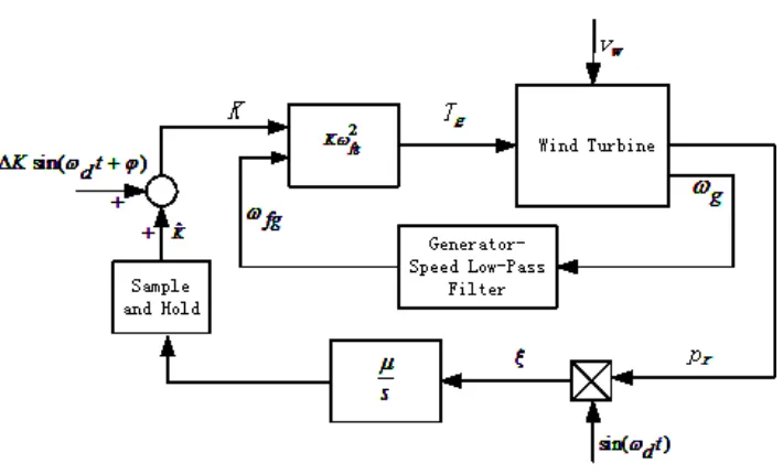
Figure 3.1 is the block diagram for torque control using conventional ESC where the torque gain K is not a constant (for standard torque control) but a variable signal tuned by ESC to maximise the rotor powerpr. In Figure 3.1,vw is the wind speed,

(52)

Figure 3.1: Block diagram of a conventional wind turbine (operating in Region 2) with a torque controller using conventional ESC.

of the sinusoidal search signal ∆Ksin (ωdt+ϕ) and needs to be very small [75],ωd

is the angular frequency of the search signal and needs to be less than the corner frequency of the generator-speed LPF [75],h_f and l_f are the corner frequencies of the HPF and LPF respectively.

Now the mechanism of torque control using the conventional ESC algorithm [75] (see Figure 3.1) is analysed. Assume that there is no wind turbulence, the relationship between the torque gain K and the rotor power pr is a static map

pr(K), and the added sinusoidal search signal ∆Ksin (ωdt+ϕ) varies much faster

than ˆK. Using the Taylor series expansion, one can derive

pr(K) =pr

ˆ

K+ ∆Ksin (ωdt+ϕ)

≈pr

ˆ

K+∂pr ∂K

ˆ

K∆Ksin (ωdt+ϕ). (3.1)

The HPF corner frequency is set to be less than ωd in order to eliminate the DC

component and pass theωd frequency component of the HPF input (3.1). Then

ξ_≈ ∂pr ∂K

ˆ

K∆Ksin (ωdt+ϕ+ϕh) sin (ωdt)

= 1 2

∂pr

∂K

ˆ

K∆K

cos (ϕ+ϕh)−cos (2ωdt+ϕ+ϕh)

(3.2)

whereϕh is the phase shift induced by the HPF. The LPF corner frequency is set

(53)

Figure 3.2: Block diagram of a conventional wind turbine (operating in Region 2) with a torque controller using SESC.

the oscillation components ofξ. Thus the integrator input is approximately 1

2 ∂pr

∂K

ˆ

K∆Kcos (ϕ+ϕh). (3.3)

Note that the actual integrator input still has small 2ωd, 3ωd, 4ωd. . . frequency

components because the LPF cannot remove them thoroughly. To guarantee correct optimum search direction, it is necessary that cos(ϕ+ϕh)>0, implying

−π

2 < ϕ+ϕh < π

2. (3.4)

Therefore, when ˆK is larger than its optimum, the integrator input (3.3) is negative, which drives the integrator output ˆKdown, and vice versa. If all the loop parameters are properly selected, the ESC loop in Figure 3.1 is stable [75]. Once the system is stable, the integrator input (3.3) is approximately 0, and thus ∂pr_∂K( ˆK) _≈ 0, which means the optimal ˆK (estimate of the torque gain) that maximises pr is acquired.

The conventional ESC loop can be simplified by replacing the LPF with a sample-and-hold (SH) block, resulting in simplified ESC (SESC) as shown in Figure 3.2. The transfer function of the SH and its magnitude are

H(s) = 1−e −sT

s , H(jω)

=T

sin ωT /2

ωT /2

(54)

−ωd

−2ωd

−3ωd

−4ωd 0 ωd 2ωd 4ωd

T

3ωd

ω(rad/s) |H(jω)|

Figure 3.3: Magnitude frequency response of the sample-and-hold.

whereT = 2π/ωdis the sample period. The magnitude frequency response of the SH

is illustrated in Figure 3.3. In the SESC loop,ξis the same as in (3.2). The integral of the 2ωd frequency component of ξ over each sample period is approximately 0,

thus the useful component of the integrator input is the same as the integrator input in the conventional ESC loop (3.3). This validates the SESC algorithm. Besides, as illustrated in Figure 3.3, the SH can attenuate high-frequency components like an LPF and removes the signals whose frequencies are integer multiples ofωd.

Considering removing both the HPF and LPF, and keeping the SH (called MSESC as seen in Figure 3.4), the integrator input becomes

ξ≈pr

ˆ

Ksin (ωdt) +

1 2

∂pr

∂K

ˆ

K∆K

cos (ϕ)−cos (2ωdt+ϕ)

. (3.6)

The integrals of both ωd and 2ωd frequency components in (3.6) over each

sam-ple period (2π/ωd) are 0. Thus, the useful component of the integrator input is

approximately

1 2

∂pr

∂K

ˆ

K∆Kcos (ϕ) (3.7)

which is almost the same as (3.3) except the absence ofϕh (the phase shift caused

by the HPF).

However, the real mapping between K and pr is not static as illustrated

in Figure 3.5: when the torque gain suddenly changes, the rotor power will not instantly reach the corresponding steady value because of the transient response of the rotor speed. Hence, the integrals of the ωd and 2ωd frequency components of

Control of large offshore wind turbines

A Thesis Submitted for the Degree of PhD at the University of Warwick

Permanent WRAP URL:

http://wrap.warwick.ac.uk/99841/

Copyright and reuse:

This thesis is made available online and is protected by original copyright.

Please scroll down to view the document itself.

Please refer to the repository record for this item for information to help you to cite it.

Our policy information is available from the repository home page.

Control of Large Offshore Wind Turbines

Xin Tong

School of Engineering

Contents

List of Tables

List of Figures

Acknowledgments

Declarations

Abstract

Abbreviations

Chapter 1

Introduction

1.1

Wind Energy

1.2

Wind Turbine System

1.3

Hydrostatic Wind Turbine

1.4

Wind Turbine Control

1.5

Motivations and Research Contributions

1.6

Thesis Outline

Chapter 2

NREL Computer-Aided

Engineering Tools and NREL

Offshore 5-MW Baseline Wind

Turbine Model

2.1

Stochastic Inflow Turbulence Simulator—TurbSim

2.2

Simulator of Wind Turbine Dynamics—FAST

2.3

Estimator of Fatigue Life—MLife

2.4

NREL Offshore 5-MW Baseline Wind Turbine Model

2.5

Conclusions

Chapter 3

Maximising Wind Power

Capture and Generation Based

on Extremum Seeking Control

3.1

Introduction

3.2

Torque Control Based on ESC