Sampling minimal, adaptive basis sets for multidimensional, nuclear quantum dynamics using simple, semi classical trajectories

(1)

warwick.ac.uk/lib-publications

A Thesis Submitted for the Degree of PhD at the University of Warwick

Permanent WRAP URL:

http://wrap.warwick.ac.uk/97217

Copyright and reuse:

This thesis is made available online and is protected by original copyright. Please scroll down to view the document itself.

Please refer to the repository record for this item for information to help you to cite it. Our policy information is available from the repository home page.

(2)

Sampling minimal, adaptive basis sets for

multidimensional, nuclear quantum dynamics

using simple, semi-classical trajectories.

Maximilian Alexander Christian Saller

Thesis submitted to the University of Warwick towards award of the degree of

Doctor of Philosophy.

Department of Chemistry

(3)

(4)

List of Tables

3.1 Input parameters and final basis set sizes for trajectory sampling calculations of the 4D pyrazine Hamiltonian, the results of which

are shown in Figures 3.4 and 3.6. . . 54

3.2 Input parameters and final basis set sizes for trajectory sampling

calculations of the 24D pyrazine Hamiltonian, the results of which

are shown in Figures 3.7 and 3.8. . . 60

3.3 Input parameters for trajectory sampling calculations of the 4D

pyrazine Hamiltonian, the results of which are shown in Figure 3.10. 64

3.4 Input parameters for trajectory sampling calculations of the 4D

3.5 Input parameters for trajectory sampling calculations of the 4D pyrazine Hamiltonian, the results of which are shown in Figure 3.12. 67

4.1 Input parameters and average total, trajectory sampled and

inher-ited basis set sizes for adaptive sampling calculations of the 4D

pyrazine Hamiltonian, the results of which are shown in Figures 4.3

and 4.4. . . 81

4.2 Mean absolute and mean absolute percentage errors for TSA and

aTSA calculations of the 4D vibronic pyrazine Hamiltonian at

vary-ing total basis set sizes with respect to exact MCTDH results.65 . . 83

inher-ited basis set sizes for adaptive sampling calculations of Model I,

the results of which are shown in Figure 4.7. . . 89

4.5 Input parameters and average total, trajectory sampled and inher-ited basis set sizes for adaptive sampling calculations of Model II,

(9)

Figure 4.9. . . 94

4.7 Input parameters for adaptive sampling calculations of the 4D pyrazine

Hamiltonian, the results of which are shown in Figures 4.11 and 4.12. 98

4.8 Input parameters and average total basis set sizes for adaptive sampling calculations of the 4D vibronic pyrazine Hamiltonian, the

results of which are shown in Figures 4.13 and 4.14. . . 101

4.9 Input parameters and average total basis set sizes for adaptive

sampling calculations of the 4D vibronic pyrazine Hamiltonian, the

results of which are shown in Figure 4.15. . . 104

4.10 Input parameters and average total basis set sizes for adaptive

sampling calculations of the 4D vibronic pyrazine Hamiltonian, the

results of which are shown in Figures 4.17 and 4.18. . . 106

inher-ited basis set sizes for adaptive sampling calculations of Model I,

using PIMD sampling trajectories, the results of which are shown

in Figure 5.2. . . 121

inher-ited basis set sizes for adaptive sampling calculations of Model II, using PIMD sampling trajectories, the results of which are shown

in Figure 5.3. . . 123

inher-ited basis set sizes for an adaptive sampling calculation of Model III,

using PIMD sampling trajectories, the results of which are shown

in Figure 5.4(c). . . 126

A.1 Number of sampling trajectories,m, used in sets of 4 calculations to

obtain the data shown in Figure 3.9, the resulting average basis set

size,Ntotaland average errors with corresponding standard deviations.150

A.2 Number of sampling trajectories, m, and sampling frequency

para-meters,ns, used in sets of 4 calculations to obtain the data shown in Figure 3.10, the resulting average basis set size,Ntotal and average

(10)

A.3 Sampling timestep duration, ∆tt, number of sampling timesteps ,nt,

and number of sampling trajectories, m, used in sets of 4

calcula-tions to obtain the data shown in Figure 3.11, the resulting average

basis set size,Ntotaland average errors with corresponding standard

deviations. . . 152

A.4 Number of sampling timesteps ,nt, and number of sampling

traject-ories, m, used in sets of 4 calculations to obtain the data shown in

Figure 3.12, the resulting average basis set size,Ntotal and average

errors with corresponding standard deviations. . . 153

A.5 Number of sampling trajectories, m, used in sets of 4 calculations with ζ = 0.95 to obtain the data shown in Figure 4.11, the

result-ing average basis set sizes and average errors with correspondresult-ing

standard deviations. . . 154

A.6 Number of sampling trajectories, m, used in sets of 4 calculations

with ζ = 0.97 to obtain the data shown in Figure 4.11, the

result-ing average basis set sizes and average errors with correspondresult-ing

standard deviations. . . 155

A.7 Number instances of the aTSA,Nb, number of sampling and

propaga-tion timesteps,nt andnp respectively, and number of sampling tra-jectories,m, used in sets of 4 calculations to obtain the data shown

in Figure 4.13, the resulting average basis set sizes and average

A.8 Number instances of the aTSA,Nb, number of sampling and

propaga-tion timesteps,nt andnp respectively, and number of sampling

tra-jectories,m, used in sets of 4 calculations to obtain the data shown

in Figure 4.14, the resulting average basis set sizes and average

A.9 Number of sampling timesteps, nt, and number of sampling traject-ories, m, used in sets of 4 calculations to obtain the data shown in

Figure 4.15, the resulting average basis set sizes and average errors

with corresponding standard deviations. . . 158

A.10 Basis set expansion parameter, γ, used in sets of 4 calculations to

obtain the data shown in Figure 4.17, the resulting average basis

(11)

(12)

List of Figures

1.1 The general mechanism of photosynthesis involves the capture of

lightvia pigments in the chlorosome antenna complex, from which

the electronic energy is then transportedvia a network of more

pig-ment molecules to the reaction centre. There, this energy is used to

drive chemical reactions such as the recycling of the coenzymes

ad-enosine triphosphate (ATP) and nicotinamide adenine dinucleotide

(NADH). . . 3

1.2 Dye sensitised solar cells typically consist of TiO2 nanoparticles to

which light-absorbing, organic dye molecules, like perylene, are

at-tached via small organic anchoring groups, which are surrounded

by an electrolyte medium. Light is absorbed by the dye molecules,

which are oxidised and the resulting electron is transferred, via the

conduction band of the TiO2 particles, to the electrode. The ion-ised dye molecules accept an electron from the electrolyte solution,

which in turn, after diffusion to the opposing electrode, is recycled

by the electrons re-entering the circuit. . . 4

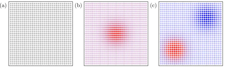
1.3 (a) Time independent quantum dynamics methods expand the

wave-function statically, (b) the expansion coefficients associated with each basis function result in the correct amplitudes in coordinate

space and (c) time evolution of the wavefunction occurs via

chan-ging of these coefficients. . . 8

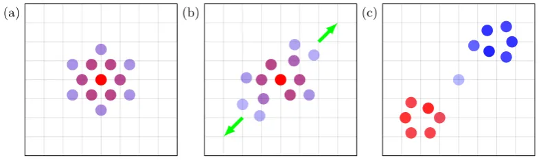
1.4 (a) The wavefunction is expanded as a small number of time-dependent

basis functions which (b) move in phase space over time. (c) As a result, basis functions continuously adapt to the changing shape of

the wavefunction. . . 9

2.1 Superposition effects of waves: (a) Constructive, in phase, and (b)

destructive, out of phase, interference of sine waves based on their phase; (c) diffraction in the context of the classic single slit

(13)

separation, Rand (b) the corresponding diabatic picture. . . 22 2.3 Multi-state quantum dynamics methods: (a) MCE trajectories,

evolve on a state averaged PES, (b) AIMS trajectories evolve

clas-sically, spawning copies of themselves to account for non-adiabatic

transitions and (c) TSH trajectories “hop” from state to state with

a probability proportional to the non-adiabatic coupling. . . 33

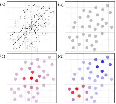
3.1 Trajectory sampling: (a) Based on the initial wavefunction, a set of

trajectories sample phase space, storing basis functions along their

path. (b) The resulting time-independent basis set is propagated

in time by (c) setting expansion coefficient to represent the initial

wavefunction and (d) evolving these coefficients variationally. . . 41

3.2 (a) Molecular structure of pyrazine, C4N2H4 and (b) diagram of

low-lying electronic states and transitions of azabenzenes. . . 47

3.3 Vibrational modes, including symmetry point groups, of pyrazine

in the S0 ground state, obtained using Møller-Plesset 2nd order

perturbation theory,107 _{with a D95}∗∗ _{basis set}108 _{in Gaussian03.}109 ₄₈

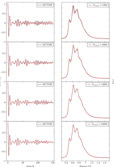
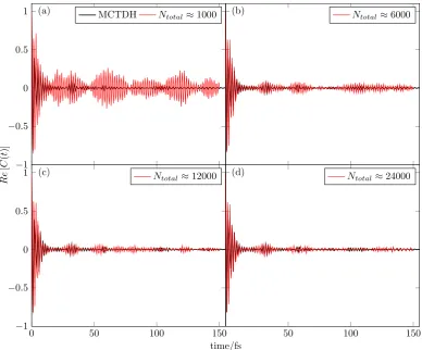
3.4 Wavefunction autocorrelation functions, C(t), and corresponding

S2 photoabsorption spectra, I(ω), for 4 trajectory sampling

calcu-lations of the 4D pyrazine Hamiltonian at varying basis set size

Ntotal, compared to MCTDH results.65 . . . 55

3.5 Effects of the dampening and sampling functions,d(t) and s(t), on

the wavefunction autocorrelation function,C(t), for the 4D pyrazine

Hamiltonian, obtained using basis set sizes of (a)Ntotal ≈1000 and

(b) Ntotal ≈24000. . . 56

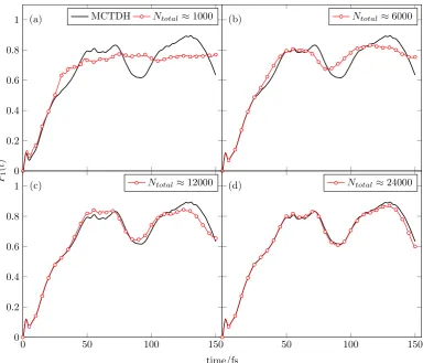
3.6 Populations of the lower S1 excited state of pyrazine, P1(t), for

the 4D pyrazine Hamiltonian, using varying basis set size, Ntotal,

compared to exact MCTDH data.65 . . . 57

3.7 Wavefunction autocorrelation functions,C(t), for the 24-dimensional

pyrazine Hamiltonian, using varying basis set sizes,Ntotal, compared

to MCTDH benchmark results.65 _{. . . 59}

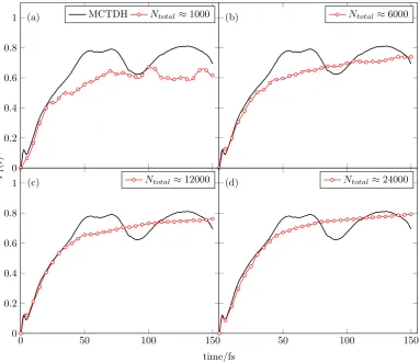
3.8 Populations of the lowerS1excited state,P1(t), for the 24-dimensional

pyrazine Hamiltonian, using varying basis set sizes, Ntotal, shown

in comparison with exact MCTDH data.65 . . . 60

3.9 (a) Mean absolute error in the P1 population of the 4D pyrazine Hamiltonian as a function of total basis set size, Ntotal, and (b)

(14)

3.10 (a) Mean absolute error in the P1 population of the 4D pyrazine

Hamiltonian as a function of the number of the sampling frequency

parameter, ns; the sampling trajectories employed, m, is

determ-ined by Eq. 3.4 and (b) corresponding mean absolute percentage

errors, using an average basis set size ofNtotal≈18000. . . 64

Hamiltonian using varying timestep durations, ∆tt, and (b)

corres-ponding mean absolute percentage errors, with an average basis set

size of Ntotal ≈18000. . . 66

Hamiltonian varying the duration of the sampling trajectories via

the total number of sampling timesteps, nt as well as the number of trajectories,m, and (b) corresponding mean absolute percentage

errors, with an average basis set size of Ntotal≈18000. . . 67

3.13 Total CPU time and (b) maximum system memory required by

trajectory sampling calculations of the 4D pyrazine Hamiltonian,

the input parameters of which are shown in Table 3.1. . . 69

4.1 The adaptive trajectory sampling algorithm: (a) Starting with a

wavefunction expanded in a basis, the number of basis functions is

minimised and their parameters optimised, resulting in (b) a more

compact wavefunction expansion. (c) Sampling trajectories are

ini-tialised from the basis functions making up the wavefunction, which

sample phase space and store basis functions along their path for a short amount of time, resulting in (d) a set of additional basis

functions, which then may be used in conjunction with the

minim-ised basis to propagate the wavefunction in time by (e) assigning all

functions coefficients and (f) propagating them in time

variation-ally. This procedure is then iterated to give long-time dynamics. . . 76

4.2 The two major stages of the MP minimisation and optimisation

algorithm: (a) From the active basis set, _{φ_}(A), the basis

func-tion possess the largest overlap with Ψ(A)is selected, removed from

{φ_}(A) and (b) optimised with respect to overlap with Ψ(A) and added to _{φ_}(M). . . 79

4.3 Populations of the lowerS1excited state of pyrazine, resulting from adaptive sampling calculations of the 4-dimensional model

(15)

sampling and adaptive sampling algorithm, with respect to MCTDH

reference results.65 _{. . . 83}

4.5 Comparison of the accuracy in the populations of the S1 state of

pyrazine for the 24-dimensional Hamiltonian for the (a)

traject-ory sampling and (b) adaptive sampling algorithm, with respect to MCTDH reference results.65 _{. . . 86}

4.6 (a) Potential energy, Vdw(q1), as a function of the tunnelling

co-ordinate of the double well benchmark and (b) V(q) for Model I, with q2 = 1 in order to demonstrate the asymmetric effect of the

harmonic bath. . . 87

4.7 Tunnelling autocorrelation functions for Model I, calculated using

the adaptive sampling algorithm with varying average total basis

set sizes,Ntotal, compared to exact CI results.119 . . . 90

4.8 Tunnelling autocorrelation functions for Model II, calculated using

the adaptive sampling algorithm with varying average total basis

set sizes,Ntotal, with respect to an exact CI benchmark.119 . . . 92

4.9 Tunnelling autocorrelation function for Model III, calculated using

(a) the adaptive sampling algorithm and (b) with the trajectory

sampling algorithm, both with respect to an exact CI benchmark.119 ₉₅

4.10 Comparison of the numbers of trajectory sampled GWP basis

func-tions and those inherited from the MP minimisation and

optimisa-tion algorithm, for the adaptive sampling calculaoptimisa-tions of the 4D pyrazine Hamiltonian, presented in Section 4.3 inputs for which are

shown in Table 4.1 and results in Figure 4.3 and Table 4.2. . . 96

Hamiltonian from adaptive sampling calculations, employing basis

sets of varying size and (b) corresponding mean absolute percentage

errors, both for MP convergence criteria ofζ = 0.95 and ζ = 0.97. . 98

4.12 Mean absolute percentage errors in the P1 population of the 4D

pyrazine Hamiltonian, comparing the performance of the aTSA and

the TSA for MP minimisation and optimisation convergence criteria

of (a) ζ = 0.97 and (b) ζ = 0.97. . . 99

Hamiltonian using varying the number of iterations of the aTSA and (b) corresponding mean absolute percentage errors, with an

(16)

Hamiltonian using varying the number of iterations of the aTSA

and (b) corresponding mean absolute percentage errors, with an

average total basis set size ofNtotal ≈9000. . . 103

Hamiltonian varying the number of sampling timesteps, nt,

result-ing in “oversamplresult-ing” and (b) correspondresult-ing mean absolute

per-centage errors, with an average total basis set size ofNtotal ≈9000. 104

4.16 Average basis set constitution, comparing average numbers of (a)

trajectory sampled, Nt, and (b) inherited basis functions, NM P,

for adaptive sampling calculations of the 4D pyrazine Hamiltonian,

varying the number of sampling timesteps, the results of which are

shown in Figure 4.15. . . 105

Hamiltonian varying the basis library expansion factor, γ, of the

MP minimisation and optimisation algorithm and (b) correspond-ing mean absolute percentage errors, with an average total basis set

size of Ntotal ≈3000. . . 107

4.18 Average basis set constitution, comparing average numbers of (a)

trajectory sampled, Nt, and (b) inherited basis functions, NM P,

for adaptive sampling calculations of the 4D pyrazine Hamiltonian,

varying the basis library expansion parameter, γ, the results of

which are shown in Figure 4.17. . . 108

4.19 (a) Total CPU time and (b) maximum system memory required by

adaptive sampling calculations of the 4D pyrazine Hamiltonian, the

input parameters of which are shown in Table 4.11. . . 110

5.1 Illustration of the PIMD equilibration algorithm: (a) Each bead is

evolved using the Velocity Verlet algorithm, (b) the centroid of the

ring is calculated based on the new bead positions, (c) each bead is

shifted by the vector connecting the new and old centroid, returning

the former to the latter. . . 120

5.2 Tunnelling autocorrelation functions for Model I, comparing the

ef-fect of using classical ((a) and (c)) and PIMD ((b) and (d)) sampling trajectories in the aTSA, varying the number of sampling

(17)

trajectories in the aTSA, varying, amongst other parameters, the

number of sampling trajectories,mand beadsn(further input

para-meters are given in Table 5.2), compared to exact CI results.119 _{. . 125}

5.4 Tunnelling autocorrelation functions for Model III, calculated using

(a) the trajectory sampling algorithm, (b) the adaptive trajectory

sampling algorithm with classical sampling trajectories and (c) the

aTSA with PIMD sampling trajectories, all compared to an exact

CI benchmark.119 . . . 127 5.5 Distribution of basis functions across the q1 tunnelling coordinate

of Model III, for a single iteration of the aTSA with (a) classical

(18)

List of Abbreviations

AI-MCE Ab initio multi-configuration Ehrenfest

AIMC Ab initio multiple cloning

AIMS Ab initio multiple spawning

ATP Adenosine triphosphate

aTSA Adaptive trajectory sampling algorithm

BEL-MCG Basis expansion leaping multi-configuration Ehrenfest

CI Configuration interaction

DD-vMCG Direct dynamics variational multi-configuration Gaussian

DOF Degree of freedom

DVR Discrete variable representation

EM Electromagnetic

G-MCTDH Gaussian multi-configuration time-dependent Hartree

GWP Gaussian wavepacket

MAE Mean absolute error

MAPE Mean absolute percentage error

MCE Multi-configuration Ehrenfest

MCTDH Multi-configuration time-dependent Hartree

MD Molecular dynamics

ML-MCTDH Multi layer multi-configuration time-dependent Hartree

MP Matching pursuit

MS Multiple spawning

NADH Nicotinamide adenine dinucleotide

OPV Organic photovoltaic

PES Potential energy surface

PIMD Path integral molecular dynamics

QTGB Quantum trajectories Gaussian basis

SOFT Split operator Fourier transform

SPF Single particle function

TDH Time-dependent Hartree

TDSCFT Time-dependent self-consistent field theory

TDSE Time-dependent Schr¨odinger equation

TISE Time-independent Schr¨odinger equation

TSA Trajectory sampling algorithm

UV Ultraviolet

(19)

(20)

Acknowledgements

First and foremost I must thank Scott Habershon, for his continued support and guidance over the last four years. I am truly grateful to him for giving me the

opportunity to work in a field both exciting and interesting to me. Over the years

he has been a truly reliable port of call for questions and advice, both guiding my

research efforts and helping me become more independent as a scientist. He has

been monumentally patient in putting up with my oddities and I truly feel that

his mentoring has given me the chance to seriously pursue a career in science.

Throughout most of my years at Warwick I was joined by a co-conspirator of sorts,

to whom I owe a non-trivial debt of gratitude. Lewis Baker has, amongst other things, been a true friend, a brother in arms and, on more than one occasion,

the voice of reason to my insanity. Whether it be on, mostly voluntary, outreach

assignments or debating intently over what some might argue are trivial or even

moot points, his company has always served to keep me sane. I seriously doubt I

will meet many people throughout my career so willing to lend an ear or give an

opinion on any matter, scientific or not.

I have been extremely lucky with respect to the working environment and my

col-leagues at Warwick. For four years I have felt that the office was not just a place of work but also a second home, full of friends who were always willing to help

and listen. So in no particular order, I would like to extend my deepest thanks to

David, Sam, Kirsten, Gareth, Anna-Laura, Jasmine and Christopher.

Finally I would like to thank the Engineering and Physical Sciences Research

Council for funding my research project, as well as the Centre for Scientific

Com-puting and the Scientific ComCom-puting Research Technology Platform for providing

computing resources and infrastructure.

An Wilhelm, Sieglinde, Harald und Elisabeth: Ohne euch g¨abe es nichts! Von

gan-zem Herzen danke ich euch für 26 Jahre Unterstützung, Förderung und Glauben

(21)

(22)

Declaration

This thesis is submitted to the University of Warwick in support of my application for the degree of Doctor of Philosophy. It has been composed by myself and has not

been submitted in any previous application for any degree. The work presented

(including data generated and data analysis) was carried out by me except in the

cases outlined below.

Maximilian Saller, July 2017

Data from the following publications was used for comparative purposes,

appro-priate citations indicating the origin in every such instance.

• A. Raab, G. A. Worth, H.-C. Meyer and L. S. Cederbaum, J. Chem. Phys., 1999, 110, 936-946

The author acknowledges the use of multi-configuration time-dependent Hartree

results for the quantum dynamics of the 4 and 24 dimensional vibronic

pyrazine Hamiltonian.

• S. Habershon, J. Chem. Phys., 2012,135, 054109

The author acknowledges the use of configuration interaction results for the

quantum dynamics of the synthetic double well tunnelling Hamiltonian.

Parts of this thesis have been published by the author:

• M. A. C. Saller and S. Habershon, J. Chem. Theo. Comput., 2015,11, 8-16

(23)

(24)

Abstract

Methods for the study of nuclear quantum dynamics can be categorised by the

nature of the basis set expansion they employ. The wavefunction can be expanded

in a static set of time-independent basis functions, the time evolution being

de-scribed solely via the expansion coefficients. Alternatively, basis functions can be

propagated in time, along with the coefficients, via equations of motion for their

parameters. Time-independent basis sets are plagued by exponential scaling, while

the equations of motion for time-dependent basis functions are challenging to in-tegrate and, if not derived variationally, can violate energy conservation laws. This

work presents a novel basis set sampling method which represents a compromise

between these two categories. A set of sampling trajectories, evolving on the

po-tential energy surface of the system, are used to place basis functions in regions of

phase space, relevant to wavefunction propagation. These functions then act as a

time-independent basis set, the wavefunction being evolved via exact, variational

equations of motion for the expansion coefficients. This approach is applied to

a challenging quantum dynamics benchmark, namely the relaxation dynamics of

photoexcited pyrazine, and yields highly encouraging results. In order to address divergence from exact dynamics at longer timescales, which is attributed to the

classical sampling trajectories being a sound approximation to quantum

propaga-tion of the wavefuncpropaga-tion only in the short-time limit, a modificapropaga-tion of this method

is proposed. Shorter iterations of trajectory sampling and wavefunction

propaga-tion are used, linked by a minimisapropaga-tion algorithm that continuously optimises the

basis set, preventing unfavourable scaling. This adaptive sampling approach is

again applied to the pyrazine benchmark with a significant increase in

perform-ance and accuracy. Highly encouraging results are also obtained for a quantum

(25)

(26)

Chapter 1 Introduction

This chapter provides an introductory overview of the field in which the work

presented herein resides. Light-matter interactions, which are the ultimate target of this research, are briefly discussed and their importance in science and

techno-logy highlighted by means of three examples. In the context of existing methods

for the study of photophysics and photochemistry, some common drawbacks and

limitations are highlighted, which this work seeks to address. Finally, the

present-ation of the remainder of this work is briefly discussed, giving an overview of the

(27)

1.1 Interactions of light and matter

Given the continued discovery of quantum phenomena, the potential applications

of the work presented herein are numerous. Quantum effects have been found

to either constitute the driving force of, or having significant impact on, physical

processes covering virtually all fields of science.1–4 However, the one field of

par-ticular interest that this work is aimed towards is photophysics and by extension

photochemistry. As suggested by their names, deriving from the Greek ph´os (ϕωςˆ ) for light, these disciplines are concerned with treating the interaction of light and

matter. Of the many physical processes known to science, there are few which

have as profound and widespread an impact as this interaction.5 _{Furthermore, as,}

at least on a timescale reasonable to human civilisation, the sun can be considered

an infinite source of energy in the form of light, the potential for technological

de-velopment, harnessing this power, certainly dwarfs that of the heavily relied upon

fossil fuels of the current era, but likely also outshines that of other renewable

energy sources.

To support these statements, the harnessing of light, both in nature, via the process of photosynthesis, and in modern technology, which aims to mimic the

former through solar cells, will be briefly discussed.

1.1.1 Photosynthesis

The definition of the term “photosynthesis” varies significantly depending on the

scientific context in which it is used, and has evolved over time, as scientific

dis-coveries have continuously broadened the array of processes it might reasonably

be applied to.6 _{For the purpose of this brief discussion, the interpretation adopted}

here will be that of a mechanism, by which an organism captures energy in the

form of light and uses it to drive chemical reactions.

Of the many approaches that may be taken to introduce the concept of photo-synthesis, the one possibly most indicative of its impact on all life on earth, and

indeed the one chosen here, is to investigate its emergence during the early stages

of earth’s planetary history and the very beginnings of life. While their origin is

one of the most highly debated topics in science, the earliest life forms, for which

no fossil record exists, are thought to have relied on the chemical environment

in which they existed, in order to survive and drive the processes of metabolism,

information storage and replication, the presence of which constitutes the most

common biological definition of life.7

Some of the earliest confirmed evidence of life are stromatolites, which are thought to be the result of photosynthetic processes. The oldest examples of

(28)

1.1. INTERACTIONS OF LIGHT AND MATTER

hν

H+

e−

ADP→ATP NADP→NADPH

etc...

6CO2+ 6H2O→C2H12O6+ 6O2

Pigments

N

-N N

N

-O

O O

O

O O

Mg2+

[image:28.595.119.515.72.296.2]

Bacteriochlorophyll-a

Figure 1.1: The general mechanism of photosynthesis involves the capture of light

via pigments in the chlorosome antenna complex, from which the electronic energy is then transportedvia a network of more pigment molecules to the reaction centre.

There, this energy is used to drive chemical reactions such as the recycling of the

coenzymes adenosine triphosphate (ATP) and nicotinamide adenine dinucleotide

(NADH).

early stage of life, photosynthesis had, in some form or another, already evolved.8

While a number of theories for the evolution of the complex metabolic pathways

and chemical structures involved with photosynthesis exist,9 _{the importance of}

photosynthetic processes in driving evolution is widely accepted. Harnessing the

sun as their major source of energy allowed organisms to become more independent

from their local chemical environment and eventually allowed them to develop more complex metabolic pathways, which in turn paved the way for more complex

life to evolve.10

The number of complex chemical and physical processes involved in

photosyn-thesis is, as for most biological phenomena that are the result of millions of years

of evolution, numerous. A general, diagrammatic outline of some of the stages of

photosynthesis is shown in Figure 1.1. For many of these processes, theoretical

and computational methods can contribute significantly towards the elucidation

of the complex underlying mechanisms. To name just one example, a key aspect of

the photosynthetic pathway involves the transfer of energy from the regions of the

organism, responsible for harvesting it, to the areas which undertake the chemical reactions that are powered by it. This excitation energy transfer has been linked

(29)

hν

3I− _I− 3

e−

Nanocrystalline TiO2

Perylene dye

Anchoring groups

Figure 1.2: Dye sensitised solar cells typically consist of TiO2 nanoparticles to

which light-absorbing, organic dye molecules, like perylene, are attachedvia small

organic anchoring groups, which are surrounded by an electrolyte medium. Light

is absorbed by the dye molecules, which are oxidised and the resulting electron

is transferred, via the conduction band of the TiO2 particles, to the electrode. The ionised dye molecules accept an electron from the electrolyte solution, which

in turn, after diffusion to the opposing electrode, is recycled by the electrons

re-entering the circuit.

dynamics model significantly helps in accounting for and expanding further on

experimental observations.12

The evolution of the ability to capitalise, via photosynthesis, on interactions

of light and matter should be considered one of the major paradigm shifting

de-velopments that allowed life to flourish, from simple, single-celled organisms, to the vast complexity with which it is observed today. As with most biological

pro-cesses that have been optimised to such an extentvia evolution, this therefore has

sufficient value to modern technology, as the next section shall discuss.

1.1.2 Solar cells

As mentioned above, the current reliance of human civilisation on a dwindling

supply of fossil fuels is almost universally accepted as unsustainable.13 _{Thus, the}

search for an alternative, cost effective renewable energy source is the focus of

major international research efforts. Given that energy in the form of sunlight is

available, essentially independent of location and more or less unlimited, photovol-taic solar cells thus theoretically constitute a potential solution to this problem.

(30)

1.1. INTERACTIONS OF LIGHT AND MATTER

basic concepts underlying natural light harvesting,14,15_{mimicking them in the}

con-text of modern technology and on a scale leading beyond pure research, towards

industrial applicability, is increasingly being considered within reach.16

The materials used in the construction of photovoltaic cells vary widely, and

significant progress has been made in increasing the efficiency for most materials

and cell architectures.17 The most common type of commercial photovoltaic cells are based on silicon which, while consistently leading other materials in terms of

ef-ficiency,18 _{is also associated with non-trivial costs. Organic photovoltaics (OPVs)}

constitute a potentially far more cost-effective alternative to the aforementioned

silicon cells, and significant research efforts are devoted to improving the efficiency

of such devices.19

Charge transfer states, one of the key features of OPVs, constitute an excel-lent example of the benefit in the design of such devices that may be gained via

theoretical study. Significant progress has been made in predicting the mechanism

by which such charge transfer states are formed using theoretical, quantum

mech-anics based models20,21 _{and the importance of quantum effects involving nuclear}

motion has been highlighted in the context of this process.21

Dye-sensitised solar cells are another example of OPVs where theoretical meth-ods have been very successful in paving the way for more efficient and less

time-consuming design of new technology. The key feature of such devices is the organic

chromophore dye, often developed by mimicking the structural and chemical

prop-erties of photosynthetical light-harvesting complexes, which is bound to

nanocrys-talline TiO2. Figure 1.2 illustrates the mechanism by which dye sensitised solar

cells harvest light and convert it to electric power. There have been a number

of very successful theoretical models proposed for these systems, including one

which allows for rapid screening of potential new dye molecules,22,23 as well as the

anchoring group used to secure it to the TiO2.

Furthermore, charge recombination, that is the migration of the electron from

the TiO2 semiconductor back to the chromophore that injected it, is the major

source of efficiency loss for dye-sensitized solar cells. A theoretical model predicting

the rate of this process for a given dye molecule has been developed,24again relying

on quantum mechanical methods to screen potential dyes. The ability to predict

the rate of charge recombination for a large number of dye molecules, without the need to experimental study, will both help reduce the costs and significantly speed

(31)

1.1.3 Ultrafast spectroscopy and the role of theory

The design of OPVs is only one example of technological processes which require

in-depth understanding of the photophysics of small organic molecules they

fea-ture. Recent advances in spectroscopy now allow increasingly detailed insights

into the photodynamics of such molecules to be gained experimentally. Modern

spectroscopic techniques allow the dynamics of atoms and molecules to be probed

on the femtosecond scale,25,26 which allows the finer details of many light-matter

interactions to be investigated. While the level of detail obtainable from such ultrafast experiments is significant and deductions can often be made with

re-gards to the underlying mechanisms, they are not able to provide insight into the

dynamics on the atomistic and sub-atomic particle scale. This is why theoretical

methods are often used in conjunction with experimental results, in order to gain a

more complete understanding of the photophysical and photochemical interactions

governing the behaviour of the system. This often involves multiple levels of one

informing the other, such as theoretical levels which are built from spectroscopic

data for a given molecule, which can then be used to further investigate and make

predictions for systems of a similar nature.

An excellent, recent example of the benefits that may be reaped from

combin-ing theoretical simulations with ultrafast spectroscopic methods is the in depth

investigation of the relaxation dynamics in ethylene.27,28 Although comparatively

simple, this system possesses two conical intersections between the ground and first

excited, π _→ π∗ electronic states, leading to non-trivial dynamics upon photoex-citation of the molecule. The first avenue of investigation concerned the lifetime

of the excited state, which had previously been both measured experimentally, at

∼50 fs,29_{and predicted using simulations, the latter however yielding a far longer} lived excited state, at 89 fs.30 _{This discrepancy between experimental results and}

theoretical predictions was attributed to two factors affecting the former. Firstly,

the energy of the pump pulse, that is the radiation used to excited the molecule

from its ground to its excited state, had previously been linked to the initial

ex-cited state geometry being close to one of the aforementioned conical intersections,

thus artificially speeding up relaxation back to the ground state. Secondly, the

probe pulse, which is used to ionise the molecule on the excited state to allow its detection, had previously involved multiphoton excitation, which significantly

increases the complexity of the theoretical model required to account for the

res-ulting dynamics.

In order to address these issues, a new set of spectroscopic measurements, using femtosecond vacuum ultraviolet pump probe spectroscopy, employing both

(32)

1.2. THEORETICAL METHODS IN PHOTOPHYSICS

theoretical simulations using on-the-fly ab initio multiple spawning (see Chapter

2 for more detail), were carried out.27 _{While resulting in far better agreement}

between the predicted excited state lifetimes, this investigation highlighted that

the photoion yield, being the measured observable in the experiment, still decays

faster than the excited state in simulations. This was linked to an energetic

condition whereby the excited molecule is not universally ionizable, even with the

higher energy probe pulse used.27

A theoretical study can, as mentioned above, also give significant insights at

the atomic and molecular scale. The investigation described above also made use

of this fact, by measuring the ratio of detected photoions. The higher energy probe

pulse employed allowed breaking of the C-C bond in the excited ethylene molecule, which allows for more in depth conclusions to be drawn about the pathways via

which the molecule decays, followingπ _→π∗ excitation, back to the ground state

state. Obtaining excellent agreement between experiment and simulation for these

ion ratios, experimental evidence for two, theoretically predicted, non-radiative

decay pathways, one involving pyramidalization the other hydrogen migration

across the C-C bond, were observed for the first time.28

The availability of quantum dynamics methods which can model light-matter

interactions for chemically interesting systems, at reasonable computational cost,

thus allows for more detailed conclusions about the detailed dynamics involved

to be drawn. This is especially relevant given the rapid advances in the field of

photoelectron spectroscopy,25,26 which allow for combined experimental and the-oretical studies like the one described above. This work seeks to address this need

by introducing a novel quantum dynamics approach, aimed at avoiding existing

issues of both limited accuracy and unfavourable computational scaling.

1.2 Theoretical methods in photophysics

Amongst the early efforts in the theoretical study of dynamic quantum effects,

a significant proportion were focused on describing the interactions of molecules

with light, particularly in the context of nuclear dynamics.31–33_{Given the wide}

sci-entific interest in light-matter interactions and the potential of theoretical methods

to complement experimental studies of systems involving the former, significant

progress has since been made in the field of nuclear quantum dynamics, which will

be discussed in more detail in Chapter 2.

When studying the interactions of light and matter on the microscopic scale,

the main challenge lies in solving the time-dependent Schr¨odinger equation (TDSE), which will be introduced again in more detail later. While classical mechanics,

(33)

[image:33.595.88.479.72.188.2]

simu-(a) (b) (c)

Figure 1.3: (a) Time independent quantum dynamics methods expand the

wave-function statically, (b) the expansion coefficients associated with each basis

func-tion result in the correct amplitudes in coordinate space and (c) time evolufunc-tion of

the wavefunction occurs via changing of these coefficients.

lated molecular processes, the nature of the electromagnetic field and its

interac-tion with molecules, which is discussed in Chapter 2 in more detail, means that for photophysical processes, quantum mechanical effects must be taken into account.

The TDSE states that

i_~∂

∂tΨ(r, t) = ˆHΨ(r, t), (1.1)

where Ψ(r, t) is the wavefunction, defined in terms of the system (nuclear and electronic) coordinates, r, at time t, ˆH is the Hamiltonian operator and _~ is the reduced Planck constant. The natural complexity of the wavefunction requires it

to be approximated via expansion in a set of mathematically simple functions, in

order to solve the TDSE. Quantum dynamics methods can thus be categorised by

the type of wavefunction expansion, oransatz, they employ and how the resulting

approximate wavefunction is then propagated in time.

1.2.1 Time-independent basis sets

As illustrated in Figure 1.3, the specific example given being the ground and ex-cited state of the harmonic oscillator, one approach is to expand the wavefunction

in terms of a large set of basis functions, the positions of which are and remain

fixed, often on a grid, throughout the time evolution. The expansion coefficients

associated with each function are then propagated in time, usually via equations

of motion derived from application of a time-dependent variational principle34–37

to the expanded wavefunction. The wavefunction ansatz for such methods may

thus be written as

Ψ(r, t)_≈ψ(r;t) =X j

(34)

1.2. THEORETICAL METHODS IN PHOTOPHYSICS

[image:34.595.121.517.72.189.2]

(a) (b) (c)

Figure 1.4: (a) The wavefunction is expanded as a small number of time-dependent

basis functions which (b) move in phase space over time. (c) As a result, basis

functions continuously adapt to the changing shape of the wavefunction.

approaches have been developed based on this rather simple scheme,38–41 _{some of}

which will later be discussed in more detail.

While the aforementioned, relative simplicity of this expansion and

propaga-tion of the wavefuncpropaga-tion is undeniable, it comes at great expense with respect to

the size of the system that may be treated. As basis functions remain fixed in

phase space and it usually is not possible to predict, without actually calculating

dynamics, which regions of phase space will be relevant to the propagation of the

wavefunction, the entirety of accessible phase space must be populated with the

basis set. This, quite straightforwardly, leads to extremely unfavourable exponen-tial scaling of the basis set size with respect to the dimensionality of the system.

Without a scheme for adaptively changing which parts of the basis set need to

be treated and which may be ignored at every step of wavefunction propagation,

which do exist and are in part discussed in Chapter 2, methods based on this

time-independent ansatz are thus limited to calculations of systems consisting of

only a few atoms.41

1.2.2 Time-dependent basis sets

Figure 1.4 shows the second common wavefunction expansion and propagation

scheme shared by many quantum dynamics approaches.42–46 _{The basis functions}

are now propagated in time, via equations of motion derived for their parameters

and expansion coefficients. The result of this is a dynamic basis set that moves in

phase space alongside the wavefunction, which may thus be written as

Ψ(r, t)_≈ψ(r;t) =X j

cj(t)φj(r;t), (1.3) where the basis functions, φj(r;t), are now time-dependent.

(35)

originates from the continuously changing distribution of basis functions in phase

space. As the basis set adapts to the shape of the wavefunction, basis functions

naturally occupy the areas of phase space where the amplitude of the wavefunction

is largest, so far fewer functions are required to describe it at any given time.

Time-dependent methods not only avoid the exponential scaling discussed above, but

in fact scale rather favourably with system size, especially when making use of

multidimensional basis functions.

There are, however, some disadvantages associated with the time propagation

of the basis functions. More specifically, the limiting factor for methods, relying on

theansatz above, are the equations of motion for the basis function parameters. If,

similarly to the expansion coefficients, these equations are derivedvia application

of a time-dependent variational principle to the TDSE featuring the expanded

wavefunction, while yielding, within the finite basis limit, formally exact results,

practically, their integration is numerically challenging, as they tend to be

ill-conditioned. This issue may be avoided by instead deriving non-variational and

thus classical or semi-classical equations of motion, however, these, in addition

to introducing yet another approximation, have been shown to violate the energy

conservation laws, implicit in the TDSE.47

This work presents an alternative method for wavefunction expansion and propagation for the purposes of quantum dynamics. While not strictly belonging

to either of the above categories, it is inspired by methods from both and is best

(36)

1.3. OVERVIEW OF THE WORK PRESENTED HEREAFTER

1.3 Overview of the work presented hereafter

The remainder of this work is structured as follows. Chapter 2 contains a brief

introduction to the theoretical background underlying the work presented in later

chapters. A number of key historical and current quantum dynamics methods,

either related to or in some way inspiring the work presented herein, are also

discussed. Chapter 3 introduces a novel scheme for sampling quantum dynamics

basis sets via simple trajectories and demonstrates their effectiveness for a chal-lenging benchmark problem. Chapter 4 addresses one of the key assumptions of

this new method, found to be the key factor limiting accuracy. A modification to

the algorithm, designed to overcome said limitation, is presented and applied to

two quantum dynamics benchmarks. Chapter 5 investigates the use of a different

type of sampling trajectories, specifically aimed at improving the description of

strong quantum effects such as tunnelling, within the novel sampling method by

applying it to a benchmark system, designed specifically with tunnelling in mind.

Finally, Chapter 6 summarises the methods and results presented in preceding

(37)

(38)

Chapter 2 Theory

This chapter lays out the essential theoretical background of the work

presen-ted thereafter, beginning with a discussion of the laws and equations of quantum

mechanics. As the goal of this work is to investigate dynamic, time-dependent

phenomena, an overview of the field of quantum dynamics is presented. Focus here is on current and historical methods, either similar in approach or somehow

inspiring the strategies presented herein. Finally, given that the phenomena

tar-geted by the work presented herein concern light-matter interactions, this chapter

concludes with a brief section on the theoretical framework underlying

(39)

2.1 Quantum mechanics

A number of experimental observations throughout the late nineteenth and early

twentieth century highlighted the fact that the well established mathematical

framework of classical mechanics was inadequate when describing the behaviour of

elemental particles, atoms and molecules. The first notion of thequantised nature

of such microscopic systems followed from experiments investigating black-body

radiation. Only discrete, not continuous, excitations of the electromagnetic field,

could account for the spectral densities, that is the relative intensity with which

individual frequencies are observed in black-body radiation at a given temper-ature. A similar observation was made when heat capacities were found to be

overestimated by a model representing each atom as a classical harmonic

oscil-lator. Again the notion of quantisation could rationalise the lower than predicted

heat capacities at low temperatures, if each harmonic oscillator required a specific,

minimum amount of energy in order to contribute to heat transfer.

Further evidence for the quantisation of the electromagnetic field was the

ob-servation of the photoelectric effect, that is the emission of an electron from a

charge surface, if exposed to ultraviolet radiation. Again this effect was only

found to occur if the radiation applied exceeded a certain frequency, however, no

such threshold was found for the intensity of radiation.

In order to explain the increasingly obvious link between electromagnetic

ra-diation and the behaviour of matter on the microscopic scale, Louis de Broglie

suggested that all moving particles were associated with a wave, the momentum,

p, of the former being linked to the wavelength,λ, of the latter via

λ= h

p, (2.1)

where h is the Planck constant. This proposed wave-like nature of matter was

soon confirmed, when electrons were observed to display diffraction (see below),

when projected at atomic crystal lattices.

Unifying observations from many experiments it was concluded that electrons,

and, as became clear over time, all of the microscopic systems alluded to above,

behave sometimes according to the familiar laws of classical mechanics, associated

with macroscopic particles, but other times akin to waves. Quantum mechanics

accounts for this duality in the behaviour of microscopic systems and links the mathematical framework governing it to macroscopic observations and

(40)

2.1. QUANTUM MECHANICS

2.1.1 Heisenberg’s uncertainty principle

The wave-like nature of microscopic particles led Werner Heisenberg to propose that if, for example, an electron with linear momentum shares some characteristics

with a moving wave, which is defined infinitely in space, then one should not be

able to know exactly both said linear momentum and the position of the electron

in space at any given time. This, eventually led to the celebrated Heisenberg

uncertainty principle which states that,

∆x∆px≥ 1

2~, (2.2)

where_~is the reduced Planck constant and ∆xis the root mean squared deviation of the positiona_{, that is to say}

∆x=p_hx2_{i − h}_x_i2_,

where the notation_hx_i denotes the average of x. This may in fact be generalised

for any two observables of the two non-commuting operators, ˆA and ˆB, such that

∆A∆B _≥ 1

2

Dh

ˆ

A,BˆiE

, (2.3)

[ ˆA,Bˆ] denoting the commutator of ˆA and ˆB, defined as

[ Â,Bˆ] = ÂBˆ₋BÂ ,ˆ

an operator being generally defined as a function mapping states, or a space of

states, to others.

2.1.2 Schr¨

odinger’s wavefunction approach

Erwin Schr¨odinger formulated a mathematical foundation of quantum mechanics,

based on the concept of wavefunctions.48–53 While the behaviour of these

wave-functions does derive from the well-established field of classical wave mechanics,

their physical interpretation in quantum mechanics is somewhat more complex. That is to say for a wavefunction, Ψ(r, t), where r are the spatial coordinates of the system and t is time, only the square of this often complex-valued function,

|Ψ(r, t)_|2 _{has physical meaning. The wavefunction does contain all information} about the system, which can be extracted using operators (for more detail see

below).

Expressing quantum mechanics based on wave mechanics allowed for the

ob-servations described above to be rationalised in terms of superposition effects. The

(41)

(a)

(b) Interfering waves Resulting signal

(c)

Figure 2.1: Superposition effects of waves: (a) Constructive, in phase, and (b) destructive, out of phase, interference of sine waves based on their phase; (c)

diffraction in the context of the classic single slit experiment.

latter are a direct result of the superposition principle,

f(x+y) =f(x) +f(y), (2.4)

f(cx) =cf(x), (2.5)

where f(x) is, by definition, a linear function and c is a scalar. In the context

of waves, superposition results in constructive or destructive interference and

dif-fraction,b _{as illustrated in Figure 2.1.}

2.1.3 Postulates of quantum mechanics

In the context of the wavefunction, the postulates of quantum mechanics are as

followsc_:

1. Any given state of a system is defined by the corresponding wavefunction

Ψ(r, t). Ψ and λΨ, where λ is a scalar, correspond to the same state and thus the wavefunction is usually chosen to be normalised, such that

Z

Ψ∗(r, t)Ψ(r, t)dτ =

Z

|Ψ(r, t)_|2dτ = 1, (2.6) b_{Depending on the field, interference and diffraction are used for superposition phenomena,}

a common distinction being based on the number of sources. That is, superposition effects due to a small number of sources are often referred to as interference, while those due to a large number of sources are called diffraction. These terms are a matter of preference only.

c_{The number, order and phrasing of these postulates vary significantly in literature, but are}

(42)

whereR

dτ refers to integration over the entire coordinate space of the

wave-function.

2. The probability dP of the particle (or system) being found in the volume elementdτ at the point (or configuration)r and at timet, can be defined as being proportional to the square of the wavefunction as

dP _{∝ |}Ψ(r, t)_|2dτ . (2.7)

This is the most common interpretation of the wavefunction, as the complex

square will be a real, positive number while Ψ itself can be complex and

negative.

3. For every observable, there exists a Hermitian operator, ˆA, satisfying

Z

a∗Abˆ dτ =

Z

b∗Aaˆ dτ ∗

, (2.8)

where a and b are functions in the domain of ˆA.d

4. The only experimentally measurable values of the observable associated with

operator, ˆA, will be the eigenvalues,a, of ˆA arising from

ˆ

AΨ =aΨ, (2.9)

assuming the system is in an eigenstate of ˆA, described by Ψ. In the case

where Ψ is not an eigenstate of ˆA, it may, because the set _{Ψj_}is complete, be expanded as

Ψ =X

j

cjΨj, (2.10)

where Ψj are eigenfunctions of ˆA with eigenvalues aj and cj are complex

expansion coefficients, determining the weight of each eigenstate. In such a case, the average value of repeated experimental measurements may be

calculated from the expectation value of the operator,

hAˆ_i=

R

Ψ∗AˆΨdτ R

Ψ∗_Ψd_τ , (2.11)

in general, which can be simplified to R Ψ∗AˆΨdτ, for any normalised

wave-function, whereR _|Ψ_|2_d_τ _{= 1.}

d_{Eq. 2.8 formally defines a symmetric operator. While the two are often used}

(43)

5. The wavefunction evolves in time according to the time-dependent Schr¨odinger

equation,

i_~∂

∂tΨ = ˆHΨ, (2.12)

where _~ is the reduced Planck constant, _~ = ₂h_π, and ˆH is the Hamiltonian operator, corresponding to the total energy of the system.

In combination with Schr¨odinger’s wavefunction based interpretation of quantum

mechanics, these postulates formally allow the behaviour of microscopic systems

to be described. Given knowledge of the wavefunction of any system, any

exper-imental observables may be calculated using the corresponding Hermitian

oper-ators. Dynamic information may be extracted by solving the partial differential

equation above and extracting the value of operators as the wavefunction evolves

in time. However, owing to the fact that Ψ fully describes the state of the system, including any observable quantities that may be measured, wavefunctions of even

the most simple molecular systems are mathematically too complex to allow Eq.

2.12 to be solved analytically. Thus a number of approximations are required.

2.1.4 Variable separation and wavepackets

In general, the wavefunction, Ψ(r, t) is a function of the system’s spatial coordin-ates, r, and time,t. A common approach in simplifying this function is to assume that solutions of the TDSE may be written as a product of functions of only spatial

coordinates and time,

Ψ(r, t) = ψ(r)χ(t). (2.13) Substituting (2.13) into (2.12) and separating the resulting equation by depend-ence on coordinates and time yields two equations for a time-independent

Hamilto-nian,

ˆ

Hψ(r) =Eψ(r), (2.14)

i_~d

dtχ(t) = Eχ(t), (2.15)

where E is the eigenvalue of ˆH, representing the total energy of the system, for

ψ(r), which are eigenfunctions of ˆH. Eq. 2.14 is the time-independent Schr¨odinger equation (TISE), which, for static systems, may be solved instead of the TDSE to

obtain time-independent properties of the system via the wavefunction.

Solving Eq. 2.15 and substituting back into (2.13) yields,

Ψ(r, t) =ψ(r)χ0exp

−i

~Et

. (2.16)

It is therefore possible to obtain dynamical information by solving the TISE and

(44)

present too much of a challenge for the TISE to be solved analytically. As noted

above, the wavefunction, and by extensionψ, refer to the same state, independent

of a scalar multiplier. χ0 is such a scalar the equation above, thus allowing it to be

absorbed into the normalisation factor of ψ such that Ψ(r, t) =ψ(r) exp(₋i

~Et).

Determining the probability density, _|Ψ(r, t)_|2_{, of this definition of the} wave-function however yields a seemingly paradoxical result.

|Ψ(r, t)_|2 =

ψ(r) exp(₋i

~Et)

∗

ψ(r) exp(₋i

~Et) = |ψ(r)|

2_. _(2.17)

The apparent lack of time-dependence in the probability density originates from

the fact that the TISE is an eigenvalue problem, that is to say that there are a

number of ψj(r) eigenstates with corresponding eigenvalues, Ej, for any given Ψ. Thus, instead of using a single such eigenstate, a linear combination may be used,e

such that

Ψ(r, t) =X j

cjψj(r) exp(−

i

~Ejt)

. (2.18)

Now the probability density will, in addition to terms originating from each spatial wavefunction, ψj(r), contain interference terms which can be thought of as being caused by the superposition of the wave-like solutions to the TDSE. For a two

eigenstate expansion for example, the wavefunction may be written as

Ψ(r, t) =c1ψ1(r) exp(−

i

~

E1t) +c2ψ2(r) exp(−

i

~

E2t), (2.19)

resulting in a probability density of

|Ψ(r, t)_|2 =_|c1|2|ψ1(r)|2+|c2|2|ψ2(r)|2+2Re

c∗₁c2ψ∗1(r)ψ2(r) exp(−

i

~(E2 −E1)t)

,

(2.20)

where now the final interference term contains the time dependence of the prob-ability density. This distribution of states with differing energies and physical

properties is termed a wavepacket.

2.1.5 Born-Oppenheimer approximation

While the time-space variable separation assumption allows for the

wavefunc-tion to be simplified, the Born-Oppenheimer approximawavefunc-tion is concerned with the

Hamiltonian operator, ˆH. In general, for a molecular system in the absence of any

perturbations, the Hamiltonian may be written as

ˆ

H =₋X

j

~2

2me∇ 2 e,j+

X

k>j

e2

|rj −rk|

−X

j

~2

2Mj∇ 2 N,j +

X

k>j

ZjZke2

|Rj −Rk|−

X

jk

Zke2

|rj −Rk|

, (2.21)

(45)

whererj andRkare the positions of electronj and nucleuskrespectively,∇2e,j and

∇2

N,k are the Laplacians with respect to the coordinates of electron j and nucleus

k respectively, Mj and Zj are the mass and charge of nucleus j, and me and e

are the mass and charge of the electron respectively. The terms in this equation

are often assigned specific symbols, based on the interactions, the contribution of

which to the total energy they represent, such that

ˆ

H = ˆTe+ ˆVe+ ˆTN + ˆVN + ˆVeN, (2.22)

where ˆTe and ˆVe are the electronic kinetic and potential energy operators, ˆTN

and ˆVN the nuclear kinetic and potential energy operators and ˆVeN the operator

describing the interactions of nuclei and electrons.

Formally the full wavefunction Ψ(r,R, t) depends explicitly on all electronic r

and nuclear R degrees of freedom (DOFs) and time t. As shown in the section above, the spatial and temporal parts of the wavefunction are often assumed to

be separable. If the time-independent wavefunction Ψ(r,R) is similarly separable between nuclear and electronic coordinates, then

Ψ(r,R) = ψ(r)χ(R), (2.23)

ψ(r) being the electronic wavefunction at a given nuclear geometry, and thus depending parametrically onR, sometimes also written asψ(r;R) andχ(R) rep-resenting the nuclear wavefunction.f _{Substituting this into the TISE yields,}

ˆ

H[ψ(r)χ(R)] = E[ψ(r)χ(R)], (2.24) for any Ψ(r,R) which is an eigenstate of the Hamiltonian. The total Hamiltonian may be separated in a number of ways, including grouping terms which depend

on the electronic coordinates r, such that ˆ

H =hTˆe+ ˆVe+ ˆVeN

i

+hTˆN + ˆVN

i

= ˆHe+ ˆHN, (2.25)

where ˆHe and ˆHN are termed the electronic and nuclear Hamiltonian respectively.

Application of ˆHeto the expanded wavefunction will, due to the separation of

elec-tronic and nuclear coordinates, yield instead of a single energy value, an elecelec-tronic

energy function, depending parametrically on nuclear coordinates,

ˆ

He[ψ(r)] =E(R) [ψ(r)]. (2.26) f_{Whilst sharing the same notation as the wavefunctions in the previous section, it should be}

Sampling minimal, adaptive basis sets for multidimensional, nuclear quantum dynamics using simple, semi classical trajectories

warwick.ac.uk/lib-publications

Sampling minimal, adaptive basis sets for

multidimensional, nuclear quantum dynamics

using simple, semi-classical trajectories.

Maximilian Alexander Christian Saller

Contents

List of Tables

List of Figures

List of Abbreviations

Acknowledgements

Declaration

Chapter 1

Introduction

1.1

Interactions of light and matter

1.1.1

Photosynthesis

1.1.2

Solar cells

1.1.3

Ultrafast spectroscopy and the role of theory

1.2

Theoretical methods in photophysics

1.2.1

Time-independent basis sets

1.2.2

Time-dependent basis sets

1.3

Overview of the work presented hereafter

Chapter 2

Theory

2.1

Quantum mechanics

2.1.1

Heisenberg’s uncertainty principle

2.1.2

Schr¨

odinger’s wavefunction approach

2.1.3

Postulates of quantum mechanics

2.1.4

Variable separation and wavepackets

2.1.5

Born-Oppenheimer approximation