Numerical simulation of continuity equations by evolving diffeomorphisms

warwick.ac.uk/lib-publications

Carrillo, Jose A., Ranetbauer, Helene and Wolfram, Marie-Therese. (2016) Numerical simulation of continuity equations by evolving diffeomorphisms. Journal of Computational Physics, 327. pp. 186-202.

Permanent WRAP URL:

http://wrap.warwick.ac.uk/83894

Copyright and reuse:

The Warwick Research Archive Portal (WRAP) makes this work by researchers of the University of Warwick available open access under the following conditions. Copyright © and all moral rights to the version of the paper presented here belong to the individual author(s) and/or other copyright owners. To the extent reasonable and practicable the material made available in WRAP has been checked for eligibility before being made available.

Copies of full items can be used for personal research or study, educational, or not-for-profit purposes without prior permission or charge. Provided that the authors, title and full bibliographic details are credited, a hyperlink and/or URL is given for the original metadata page and the content is not changed in any way.

Publisher’s statement:

© 2016, Elsevier. Licensed under the Creative Commons Attribution-NonCommercial-NoDerivatives 4.0 International http://creativecommons.org/licenses/by-nc-nd/4.0/

A note on versions:

The version presented here may differ from the published version or, version of record, if you wish to cite this item you are advised to consult the publisher’s version. Please see the ‘permanent WRAP URL’ above for details on accessing the published version and note that access may require a subscription.

EQUATIONS BY EVOLVING DIFFEOMORPHISMS

JOS ´E A. CARRILLO∗, HELENE RANETBAUER‡, AND MARIE-THERESE WOLFRAM§

Abstract. In this paper we present a numerical scheme for nonlinear continuity

equa-tions, which is based on the gradient flow formulation of an energy functional with respect to the quadratic transportation distance. It can be applied to a large class of nonlinear continuity equations, whose dynamics are driven by internal energies, given external po-tentials and/or interaction energies. The solver is based on its variational formulation as a gradient flow with respect to the Wasserstein distance. Positivity of solutions as well as energy decrease of the semi-discrete scheme are guaranteed by its construction. We illustrate this properties with various examples in spatial dimension one and two.

Keywords: Lagrangian coordinates, variational scheme, optimal transport, finite ele-ment, implicit in time discretization

1. Introduction

In this work we propose a numerical method for solving nonlinear continuity equations of the form:

∂tρ=−∇ ·[ρv] := ∇ ·[ρ∇(U0(ρ) +V +W ∗ρ)] (1a)

ρ(0,·) =ρ0, (1b)

whereρ=ρ(t, x) denotes the unknown time dependent probability density andρ0 =ρ0(x)

a given initial probability density on Ω ⊆ _Rd_{. The function U :}

R+ → R is an internal

energy, V = V(x) : _Rd → _R a given potential and W = W(x) : _Rd → _R an interaction potential. Equation (1) can be interpreted as a gradient flow with respect to the Euclidean Wasserstein distance of the free energy or entropy

E(ρ) =

Z

Rd

U(ρ(x))dx+

Z

Rd

V(x)ρ(x)dx+ 1

2

Z

Rd×Rd

W(x−y)ρ(x)ρ(y)dxdy.

∗_{Department of Mathematics, Imperial College London, London SW7 2AZ, UK;}

email: [email protected]

‡_{Radon Institute for Computational and Applied Mathematics, Austrian Academy of Sciences,}

Al-tenberger Strasse 69, 4040 Linz, Austria; email: [email protected]

§_{Mathematics Institute, University of Warwick, Coventry CV4 7AL, UK and Radon Institute for}

Com-putational and Applied Mathematics, Austrian Academy of Sciences, Altenberger Strasse 69, 4040 Linz, Austria;

email: [email protected]

1

Then the velocity field v = v(t, x) corresponds to v = −∇δE

δρ, and the free energy is

dissipated along the trajectories of equation (1), i.e.

d

dtE(ρ)(t) = −D(ρ)≡ −

Z

Rd

|v(t, x)|2_{ρ(t, x)dx.}

HereD(ρ) denotes the so called entropy dissipation functional.

The gradient flow formulation detailed above provides a natural framework to describe the evolution of densities and it has been successfully used to model transportation pro-cesses in the life and social sciences. Examples of it include the heat equation with

U(s) = slns, V = W = 0 or the porous medium and fast diffusion equation with

V = W = 0 and U(s) = sm/(m −1) for m > 1 and 0 < m < 1 respectively. If the dynamics are in addition driven by a given potentialV, we refer to (1) as a Fokker-Planck type equation. Gradient flow techniques have also been applied to aggregation equations, which correspond to (1) for a given interaction potential W and U = V = 0. These models appear naturally to describe spatial shapes of collective dynamics in general and in particular for animal swarms, for example the motion of bird flocks or fish schools, cf. [46, 50, 51, 27]. See also the reviews [42, 19] and the references therein. Applications in physics include the field of granular media [25, 52] or material sciences [37]. A common assumption in collective dynamics is that W is a radial function, i.e. W =W(|x|). Hence interactions among individuals depend on their distance only. The interaction dynamics are often driven by attractive and repulsive forces, mimicking the tendency of individuals to stay close to the group but maintain a minimal distance. A popular choice among attractive-repulsive potentials is the Morse potential, that is

W(r) =−CAe−r/lA +CRe−r/lR,

where CA and CR are the attractive and repulsive strength and lA, lR their respective

length scales, see [44, 8, 22, 20, 43, 1]. Also power-law potentials of the form

W(r) = |r|

a

a −

|r|b

b , a > b,

have been used thoroughly. We refer to the works of [43, 6, 5, 30, 31] for more details. Purely attractive potentials are often of the formW(r) = |r|a_{, a >0. In this case the}

den-sity of particles collapses in finite or in infinite time and converges to a Delta Dirac located at the center of mass for certain range of values, see [9, 39, 38, 16]. Finally, aggregation-diffusion equations, in which both the linear or nonlinear aggregation-diffusion term modelling repulsion and the aggregation term modeling attraction are present, are ubiquitous models in physics and biology, including all different versions of the parabolic-elliptic Keller-Segel model for chemotaxis, see for instance [36, 54, 12, 10, 11, 57] and the references therein.

advantages such as build-in positivity and free-energy decrease. There has been an increas-ing interest in the development of such methods in the last years, for example variational Lagrangian schemes such as [34, 33, 56, 28, 10, 45, 21, 41] or finite volume schemes as in [23]. The common challenge of all methods is the high computational complexity, often restricting them to spatial dimension one. They involve for example the solution of the Monge-Kantorovich transportation problem between measures, which require the compu-tation of the Wasserstein distance. In 1D the Wasserstein distance corresponds to the

L2 distance between inverses of the distribution functions. In higher space dimensions its computation involves the solution of an optimal control problem itself, which poses a significant challenge for the development of numerical schemes. There are few results on the numerical analysis of these schemes, for example Matthes and co-workers provided first results on the convergence in 1D in [45]. Recent works [7] are making use of recent de-velopments in the fast computation of optimal transportation maps to discretize the JKO steps in the variational scheme.

Many of the Lagrangian methods are based on the “discretize-then-minimize” strategy, see for example [56, 28, 45, 7, 21, 41]. However, we follow closely the advantage of the 1D formulation in terms of the pseudo-inverse function, see also [34, 33, 10], which corresponds to a “minimize-then-discretize” strategy. In higher dimensions, this strategy is based on the variational formulation of (1) for a diffeomorphism mapping the uniform density to the unknown density ρ. Evans et al. proved in [29] that this approach corresponds to a class of L2-gradient flows of functionals on diffeomorphisms. This equivalent formulation served as a basis for the numerical solver of Carrillo and Moll [26], which uses the vari-ational formulation and an explicit in time as well as a finite difference discretization in space. We shall follow their approach but propose an implicit time stepping and a spatial discretization, which is based on finite differences in 1D and finite elements in 2D. We would like to mention that the our scheme coincides with the implicit in time finite differ-ence discretization of the pseudo-inverse function proposed by Blanchet et al. for the 1D Patlak-Keller-Segel model, see [10]. The finite element discretization allows us to consider more general computational domains as well as triangular meshes. This is advantageous in the case of radially symmetric solutions, which develop asymptotically for large times for many types of aggregation-diffusion equations. Due to the implicit in time stepping no CFL condition as in [26] is necessary. Moreover, if our dicretization were convergent for the implicit semidiscretization of the PDE system satisfied by the diffeomorphisms, the numerical scheme would be convergent for an exact JKO step of the the variational scheme.

2. _{Gradient flow formulation}

We start by briefly reviewing the variational formulation of (1) as a gradient flow with respect to a particular distance and energy. Let us consider the quadratic Wasserstein distance between two probability measuresµ∈ P(_Rd) and ν ∈ P(_Rd) given by

d2_W(µ, ν) := inf

T:ν=T#µ Z

Rd

|x−T(x)|2_dµ(x),

for any µ absolutely continuous with respect to Lebesgue, see [55] for a general definition and its properties. It is well known that solutions of (1) can be constructed via the so-called JKO scheme, see [40], which corresponds to solving

ρn_∆+1_t ∈arg min

ρ∈K

1 2∆td

2 W(ρ

n

∆t, ρ) +E(ρ)

, (2)

for a fixed time step ∆t > 0 and K = {ρ ∈ L1₊(_Rd) : R

Rdρ(x)dx = M,|x|

2_{ρ ∈ L}1₍

Rd)}.

Hence (2) can be understood as a time discretization of an abstract gradient flow equation in the space of probability measures. It has been proven that solutions of (2) converge to the solutions of (1) first order in time, see [40, 48, 55, 2] for more detailed results on the analysis.

Evans et al. [29] showed that there is a connection between the theory of steepest descent schemes with respect to the Euclidean transport distance and the L2_{-gradient flows of}

polyconvex functionals of diffeomorphisms. Since this formulation serves as a basis of the proposed numerical solver, we will review the main results in the following. Let ˜Ω be a smooth, open, bounded and connected subset of _Rd and Ω be an open subset of _Rd. Let

D denote the set of diffeomorphisms from Ω to ¯¯˜ Ω, mapping ∂Ω onto˜ ∂Ω. Furthermore we consider the energy functional:

I(Φ) =

Z

˜ Ω

Ψ(detDΦ)dx+

Z

˜ Ω

V(Φ(x))dx+1

2

Z

˜ Ω×Ω˜

W(Φ(x)−Φ(y))dxdy,

where Ψ(s) = sU 1_s. Ambrosio et al [3] clarified even further this subtle relation found in [29], by showing that the L2_{-gradient flow of I(Φ) with V =W = 0 given by}

Φn_∆+1_t ∈arg min

Φ∈D

1 2∆tkΦ

n

∆t−ΦkL2_(Ω)+I(Φ)

(3)

is well defined and converges to the solutions of the nonlinear PDE system

∂Φ

∂t =∇ ·

Ψ0(detDΦ)(cofDΦ)T,

whereDΦ is the Jacobian matrix of Φ and cofDΦ the corresponding cofactor matrix. This connection was generalized subsequently in [26] to the case of interaction and potential energies, leading to the nonlinear PDE system

∂Φ

∂t =∇ ·

Ψ0(detDΦ)(cofDΦ)T− ∇V ◦Φ− Z

˜ Ω

The diffeomorphism Φ maps a given reference density, for instance the uniform density on a reference domain ˜Ω, to the unknown density ρ in Ω. Therefore the density ρ ∈ K can be calculated via ρ = Φ#LN _{for every diffeomorphism Φ ∈ D, assuming that |Ω˜| = M,}

where LN _{denotes the N-dimensional Lebesgue measure on the reference domain ˜Ω. An}

equivalent formulation in the case of a sufficiently smooth diffeomorphism Φ is given by

ρ(Φ(x)) det(DΦ(x)) = 1. (5)

Hence we can interpret equation (4) as the Lagrangian representation of the original non-linear continuity equation (1) in Eulerian coordinates.

3. Spatial and temporal discretization of the Lagrangian representation

In this section we present the details of the spatial and temporal discretization of equa-tion (4), focusing on the implicit in time scheme and the subsequent finite dimensional approximation of the nonlinear semi-discrete equations. The latter is discretized by a fi-nite difference scheme in 1D and a fifi-nite element method in 2D. In the following we shall only present the finite element discretization of (4), since the 1D finite difference scheme is detailed in [10, 26] already.

Let ∆tdenote the discrete time step,tn+1 = (n+ 1)∆tand Φn+1the solution Φ = Φ(t, x) at timetn+1_{. Then the implicit in time discretization of (4) reads as}

Φn+1_−Φn

∆t =∇ ·[Ψ 0

(detDΦn+1)(cofDΦn+1)]

− ∇V(Φn+1)−

Z

˜ Ω

∇W(Φn+1(x)−Φn+1(y))dy. (6)

Let us consider test functions ϕ=ϕ(x)∈ H1_{( ˜Ω). Then the nonlinear operator F defined}

via (6) is given by:

F(Φ, ϕ) = 1

∆t Z

˜ Ω

(Φn+1−Φn)ϕ(x)dx+

Z

˜ Ω

Ψ0(detDΦn+1)(cofDΦn+1)∇ϕ(x)dx

+

Z

˜ Ω

∇V(Φn+1)ϕ(x)dx+

Z

˜ Ω

Z

˜ Ω

∇W(Φn+1(x)−Φn+1(y))dy

ϕ(x)dx.

(7)

We use lowest order H1 conforming finite elements, also known as hat functions, for the discretization of Φ, more precisely piece-wise linear functions. The discrete diffeomorphism Φh = Φh(x1, x2) can be written as

Φh(x1, x2) = X

j

Φ1_j

Φ2 j

!

ϕj(x1, x2),

drop the subscript h to enhance readability in the following). To do so, we calculate the Jacobian matrixDF of (7) and determine the Newton update Υn+1,k+1 _via

DF(Φn+1,k, ϕ)Υn+1,k+1 =−F(Φn+1,k, ϕ),

for all test functionsϕ(x)∈H1_{( ˜Ω). The index k corresponds to the Newton iteration and} n to the temporal discretization. Note that the Jacobian matrix Υn+1,k+1 _{is a full matrix}

and has no sparse structure due to the convolution operator W. The Newton updates are calculated via

Φn+1,k+1 = Φn+1,k +αΥn+1,k+1,

where α is a suitable damping parameter. The Newton iteration is terminated if

|F(Φn+1,k+1, ϕ)| ≤1 orkΦn+1,k+1−Φn+1,kk ≤2,

with given error bounds 1 and 2. Note that due to the implicit in time discretization no

CFL type condition for the time step ∆t, as in [26], is necessary.

The presentedL2_{-gradient flow (3) is only valid if the total mass is conserved. This can}

be implemented by adopting the image domain in 1D or by considering equation (1) with no flux boundary conditions in 2D, i.e.

v·n= 0 on ∂Ω,

where n denotes the outer unit normal vector on the boundary ∂Ω and v is given by (1). We shall only consider diffeomorphisms which map ∂Ω onto˜ ∂Ω without rotations as in [26]. Then the corresponding natural boundary conditions for the equation in Lagrangian formulation are given by

nT(cofDΦ)T∂Φ

∂t = (cofDΦ)n·

∂Φ

∂t = 0. (8)

Note that the boundary conditions (8) have to be checked separately for every computa-tional domain, see for example [26] for the discussion of appropriate boundary conditions in the case of the unit square. In the case of a circle with radius R we have:

1

R

x1

x2

∂Φ2

∂x2 −

∂Φ1 ∂x2

−∂Φ2 ∂x1

∂Φ1 ∂x1

∂Φ1 ∂t ∂Φ2

∂t

= 0.

Using radial coordinatesx1 =Rcosθ and x2 =Rsinθ, we obtain:

cosθ(∂Φ1

∂t

∂Φ2

∂x2

− ∂Φ2

∂t

∂Φ1

∂x2

) + sinθ(−∂Φ1 ∂t

∂Φ2

∂x1

+∂Φ2

∂t

∂Φ1

∂x1

) = 0.

Since ∂Φ1

∂θ =−sinθ ∂Φ1

∂x = cosθ ∂Φ1

∂x2, we conclude that

sinθ∂Φ2 ∂t

∂Φ1

∂x1

+ cosθ∂Φ1 ∂t

∂Φ2

∂x2

Hence, in the case of a circle equation (9) is equivalent to (8).

If we assume that the boundary of ˜Ω is mapped onto the boundary of Ω, the corresponding diffeomorphism is given by

Φ1(t, x) = Φ2(t, x) = Id,

which implies that ∂Φ1

∂t =

∂Φ2

∂t = 0 on the boundary. This choice ensures that the equivalent

boundary conditions given by (9) are satisfied.

4. Pre-processing and post-processing: calculating the initial diffeomorphism and the final density

The discretization of theL2_{-gradient flow formulation involves several pre- and}

postpro-cessing steps. First the initial diffeomorphism Φ0 has to be computed for a given initial

densityρ0. The postprocessing step corresponds to calculate the density ρT from the final

diffeomorphism ΦT . We shall detail these two steps in the following.

4.1. Pre-processing: Let ρ0(x) be a given smooth initial density with R

Ωρ0(x)dx = M

and denote by Φ0 = Φ0(x) := Φ(0, x) the corresponding diffeomorphism. Then the initial

diffeomorphism Φ0 :Ω¯˜ →Ω satisfies¯

ρ0(Φ0(x)) detDΦ0(x) = 1. (10)

Depending on the discretization of ˜Ω different approaches can be used to determine Φ0(x)

from a given ρ0(x). In the case of an equidistant mesh of squares or rectangles, one can calculate the initial diffeomorphism by solving a one-dimensional Monge-Kantorovich problem in x1 direction and subsequently a family of Monge-Kantorovich problems in the x2 direction, cf. [35, 26].

However this approach is not possible in case of general quadrilateral or triangular meshes. In this case different strategies can be used: either based on the Monge Am-pere equation (giving the optimal transportation plan in case of quadratic cost), Knote theory or density equalizing maps. We shall follow the latter, which is based on an idea of Moser [47] that was further studied by Avinyo and co-workers in [4]. It is based on the idea of constructing the initial diffeomorphism from solutions of the heat equation with homogeneous Neumann boundary conditions. This approach was also used in cartography to calculate density equalizing maps, cf. [32]. Its advantage is its flexibility - it can be used for general computational domains and their respective discretizations since it only requires the efficient solution of the heat equation.

Consider the heat equation written as a continuity equation on a bounded domain Ω⊂

R2 as

∂ρ

∂t + div(ρv) = 0, with v =− ∇ρ

ρ , (11)

and initial datum ρ(0, x) =ρ0(x) as well as homogeneous Neumann boundary conditions.

v = −∇ρ

ρ towards the constant density ¯ρ = 1 |Ω|

R

Ωρ0(x)dx as t → ∞. Hence the velocity

field can be calculated by solving the heat equation until equilibration. Then the cumulative displacement x(t) of any point at time t is determined by integrating the velocity field, which corresponds to solving

x(t) =x(0) +

Z t

0

v(t0,x(t0))dt0.

As t → ∞, the set of such displacements for all points x = x(t) in Ω, that is the grid points of the computational mesh, defines the new density-equalized domain. Note that we actually need to determine its inverse, since we need to find the map which maps the constant density to the initial densityρ0. Hence we solve:

x0(t) = v(t0,x(t0)) =−∇ρ(t,x(t))

ρ(t,x(t)) (12a)

x(T) = x1, (12b)

for all mesh points x1 ∈ Ω. This corresponds to the solution of the integral equation

x(0) =x(T)−RT

0 v(t,x(t))dt. Altogether the pre-processing consists of two steps:

(1) Solve the heat equation with Neumann boundary conditions for an initial datum

ρ0 = ρ0(x) until equilibration. The time of equilibration corresponds to the time

where the L2_{−norm between two consecutive time steps is less than 10}−6_.

(2) Starting with a given mesh at time t = T calculate the initial diffeomorphism by solving (12) backward in time. Then the initial diffeomorphism is given by Φ0(x1) = x(0).

Remark 4.1. Note that the one could also use the initial densityρ0 as a reference measure,

then the initial diffeomorphism φ0 is the identity map. In this case equation (5) would read

as

ρ(Φ(x)) det(DΦ(x)) =ρ0(x).

4.2. Post-processing: The post-processing step corresponds to calculate ρT := ρ(t = T, x) given the final diffeomorphism ΦT := Φ(t=T, x). Since we expect numerical artifacts

in case of compactly supported and measure valued solutions we solve a regularized version of (5) (in 2D) given by:

ε∆ρT(ΦT(x)) +ρT(ΦT(x)) =

1 detDΦT(x)

with 0< ε1. (13)

5. _{Numerical simulations}

In this section we illustrate the behavior of the numerical solver with simulations in spatial dimension one and two. The 1D simulations are based on a finite difference dis-cretization, in 2D we use finite elements. The respective solvers are based on Matlab in 1D and on the finite element package Netgen/NgSolve in 2D. In the following we illustrate the flexibility of our approach with various simulations for a large class of PDEs. We start by summarizing all steps of the numerical solver in Algorithm 1.

5.1. Numerical simulations in spatial dimension one. If not stated otherwise we initiate all numerical simulations with a Gaussian of the form:

ρ0(x) =

M √

2πσ2e

−x2

2σ2 (14)

with M, σ > 0. Note that R_−∞∞ ρ0(x)dx = M. We perform our simulations on a bounded

domain ˜Ω = [0,M˜], where ˜M is the approximate value of R

Ωρ0(x)dx. Hence, the initial

diffeomorphism Φ0 is defined on ˜Ω.

5.1.1. Nonlinear diffusion equations. In our first example we illustrate the behavior of our scheme for the Porous medium equation, that is U(s) = _m1₋₁sm_{, m > 1 and V =W = 0.}

Let Ω = [−1,1] denote the computational domain discretized into 501 intervals of size ∆x = 2

501. The initial density is given by a Barenblatt Pattle profile (BPP) at time t0 = 10−3, i.e.

ρ0(x) =

1

tα 0

c−αm−1

2m

x2

t2α 0

m1−1

+ ,

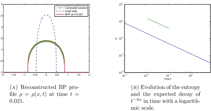
where α = _m1₊₁ and c is chosen such that R₋1₁ρ0(x)dx = 2. The discrete time steps are set to ∆t = 10−5. We consider the cases m = 2 and m = 4. Figures 1 and 2 show the density profilesρat timet= 0.021 as well as the evolution of the free energy in time, which decays like t−α(m−1), cf. [53]. As seen from Figures 1b and 2b, these decays (indicated by the green lines) are perfectly captured by the scheme validating the chosen discretization. Note that the boundary points of the support are calculated using an explicit one-sided difference scheme of the velocity as proposed by Budd et al., see [14]. In particular, writing the porous medium equation as

ρt+∇ ·(ρv) = 0

with the velocity v = − m m−1(ρ

m−1₎

x leads to the approximation Φn+1 = Φn+ ∆tv at the

boundary points. When determining ρx we assume that the density at the boundary of

the support equals zero.

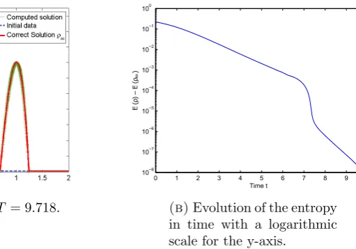
5.1.2. Fokker-Planck type equations. Next we study the behavior of a nonlinear Fokker-Planck equation in the case of an internal energy U(s) = νs_mm, m > 1 and a double-well confining potential V(x) = x₄4 − x2

2 . Let Ω = [−2,2] be the computational domain

discretized into 501 intervals of size ∆x = ₅₀₁4 . The initial density is given by (14) with

Algorithm 1 Letρ0 =ρ0(x) be a given initial density with R

Ωρ0(x)dx=M and Ω = [a, b]

or Ω = [a, b]×[c, d].

(1) Determine the initial diffeomorphism

(a) 1D: Define the initial diffeomorphism Φ0 : ˜Ω = [0, M] → [a, b] by: for every

discretization point xi ∈[0, M] solve the one-dimensional Monge-Kantorovich

problem for Φi = Φ(xi):

Z Φi

a

ρ0(y)dy=xi,

using Newton’s method.

(b) 2D: Follow the two-step algorithm outlined in Section 4.1: Solve the heat equation∂tρ= ∆ρwith homogeneous Neumann boundary conditions using an H1 _{conforming finite element method of orderp= 6 until equilibration at time} t =T. Determine the initial diffeomorphism by transporting each mesh point of the computational mesh V(T) = (xV

1(T),xV2(T))∈ V backward in time

x(0) =x(T)−

Z T

0

v(t,x(t))dt, v(t,x(t)) =−∇ρ(t,x(t))

ρ(t,x(t)) .

(2) At every time steptn+1= (n+ 1)∆t in t∈(0, T] solve

(a) 1D: the implicit equation (6) using Newton’s method and finite difference dis-cretization.

(b) 2D: the nonlinear operator equation F(Φ, ϕ) = 0, given by (7) using Newton’s method and a spatial discretization of H1 conforming finite elements of order

p= 1.

(3) Recover the final density ρ=ρ(T) by

(a) 1D: calculating the final density at every discrete point Φi = Φ(xi) from the

relation

ρ(Φ(x)) = 1

detDΦ(x).

(b) 2D: solving the regularized equation

ε∆ρ(Φ(x)) +ρ(Φ(x)) = 1

detDΦ(x)

on the transformed mesh N using H1 conforming elements of order p= 4.

states are given by

ρ∞(x) =

1

ν (C(x)−V(x))

1

m−1

+ , (15)

where C =C(x) is a piecewise constant function possibly taking different values on each connected part of the support, cf. [23]. The density at time T and the entropy decay with respect to ρ∞ are illustrated in Figure 3. We always choose T in Section 5.1 as the time

−2 −1.5 −1 −0.5 0 0.5 1 1.5 2 0

1 2 3 4 5 6

Computed solution Initial data BPP at t=0.021

(a) Reconstructed BP pro-file ρ = ρ(x, t) at time t = 0.021.

10−3 10−2 10−1 100

10−1 100 101

102

Time t

E

(b)Evolution of the entropy and the expected decay of t−α in time with a logarith-mic scale.

Figure 1. Solution of the PME for m= 2 after 2000 time steps.

−2 −1.5 −1 −0.5 0 0.5 1 1.5 2

0 0.5 1 1.5 2 2.5 3

Computed solution Initial data BPP at t=0.021

(a) Reconstructed BP

pro-file ρ = ρ(x, t) at time t = 0.021.

10−3

10−2

10−1

100 10−2

10−1 100 101 102

Time t

E

(b)Evolution of the entropy

and the expected decay of t−3αin time with a logarith-mic scale.

Figure 2. Solution of the PME for m= 4 after 2000 time steps.

and refer to ρ at time T +t0 for t0 = 500∆t as the steady state ρ∞. We observe that the

(a) Densityρat timeT = 9.718.

0 1 2 3 4 5 6 7 8 9

10−8 10−7 10−6 10−5 10−4 10−3 10−2 10−1 100

E

(

ρ

)

−

E

(

ρ∞

)

Time t

(b)Evolution of the entropy in time with a logarithmic scale for the y-axis.

Figure 3. Solution of the nonlinear Fokker-Planck equation form = 2 and

ν = 0.05.

If the confining potential is chosen as the harmonic potential V(x) = x₂2, the steady state is also given by (15), cf. [17]. The convergence towards the steady state is exponen-tial, more precisely Carrillo et al. [17] showed that the distance towards equilibrium, i.e.

d2_W(ρ(t), ρ∞), converges likeO(e−(m+1)t) since the initial data has zero center of mass. The

same convergence behavior can be observed in the numerical simulations, see Figure 4a and 4b. Note that the rate of convergence in relative energy in Figure 4b coincides with the rate of convergence ofd2_W(ρ(t), ρ∞).

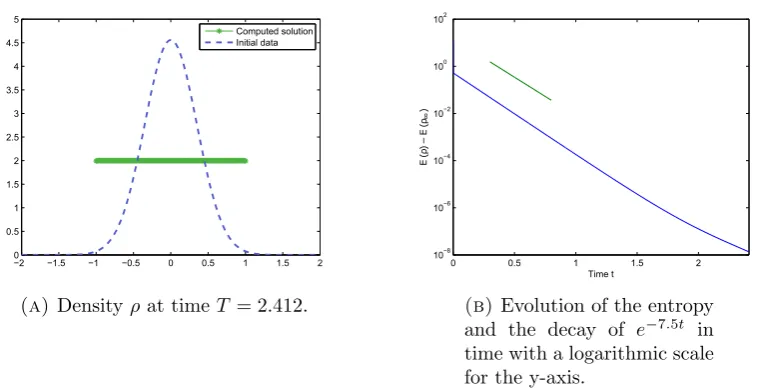
5.1.3. Aggregation equations. Next we consider aggregation potentials of the form

W(x) = |x|

a

a −

|x|b

b , (16)

for a > b ≥ 0 using the convention that |x|0_{/0 = ln|x|. The set of stationary states of}

these equations can be quite complex, see [43, 6, 5], depending on the dimension. In one dimension with a = 2 and b = 1 the steady state profiles are constant on an interval, cf. [30, 31], for a= 2, b= 0 they correspond to the semicircle law, cf. [49, 24].

Let a = 2, b = 1 and set Ω = [−2,2] split into 201 intervals of size ∆x = ₂₀₁4 . The initial datum is given by (14) with σ = 0.35 and M = 4. The discrete time steps are set to ∆t = 10−3_{. Figure 5 shows the computed solution at time T and the entropy decay with}

respect toρ∞. The numerical simulations confirm the theoretical results, i.e. the computed

stationary profile corresponds to the constant density ρ∞(x) = 2 for all x ∈[−1,1]. Note

−2 −1.5 −1 −0.5 0 0.5 1 1.5 2 0 0.2 0.4 0.6 0.8 1 1.2 1.4 1.6 1.8

2 Computed solution Initial data Correct Solutionρ∞

(a) Densityρat timeT = 3.172.

1.4 1.6 1.8 2 2.2 2.4 2.6 2.8

10−7 10−6 10−5 10−4 10−3 10−2 10−1 100 E ( ρ ) − E ( ρ∞ ) Time t N=101 N=301 N=501 line of slope−3

(b) Semi-log error plot at time t for different values for N = _∆|Ω_x| with respect to the steady state.

Figure 4. Solution of the nonlinear Fokker-Planck equation form = 2 and

ν = 2.

−2 −1.5 −1 −0.5 0 0.5 1 1.5 2

0 0.5 1 1.5 2 2.5 3 3.5 4 4.5 5 Computed solution Initial data

(a) Densityρat timeT = 2.412.

0 0.5 1 1.5 2

10−8 10−6 10−4 10−2 100 102 Time t E ( ρ ) − E ( ρ∞ )

(b)Evolution of the entropy

and the decay of e−7.5t _in time with a logarithmic scale for the y-axis.

Figure 5. Solution of the aggregation equation with potential (16) (a= 2,

b= 1).

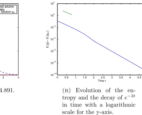
In the case a = 2, b = 0 we set Ω = [−6,6] split into 501 intervals of size ∆x = ₅₀₁12. Then the unit-mass steady state is given by

ρ∞(x) =

( 1 π

√

2−x2_{, |x| ≤}√_2,

This result is confirmed by the numerical simulations illustrated in Figure 6 for an initial datum ρ0 given by (14) with σ = 1 and M = 1. It is known that the solutions decay

−3 −2 −1 0 1 2 3

0 0.5 1 1.5

Computed solution Initial data Correct Solutionρ∞

(a) Densityρat timeT = 4.891.

0 0.5 1 1.5 2 2.5 3 3.5 4 4.5 10−10

10−8 10−6 10−4 10−2 100 102

Time t

E

(

ρ

)

−

E

(

ρ∞

)

(b) Evolution of the

en-tropy and the decay ofe−3t in time with a logarithmic scale for the y-axis.

Figure 6. Solution of the aggregation equation with potential (16) (a= 2,

b= 0).

in dW toward the corresponding stationary states ρ∞ exponentially fast. We observe that

behavior at the level of the relative energy with numerical rates of decay given by 7.5 and 3 approximately in Figures 5b and 6b.

5.1.4. Modified Keller-Segel model. In our final example we consider a modified Keller-Segel (KS) model. It is well known that solutions of the classical Keller-Keller-Segel may blow up in finite time in space dimensions d ≥ 2, see cf. [15, 10]. The same behavior can be observed in 1D by using the corresponding 2D interaction potential instead. Then the modified KS model reads as:

∂tρ=∇ ·(ρ(∇(lnρ+W ∗ρ))),

W = χ

dπ ln|x|,

ρ(x,0) = ρ0 ≥0.

(17)

The blow-up behavior depends on the initial mass M0 = R_Ωρ0(x)dx. If M0 < Mc, where χMC = 2d2πdenotes the critical mass, the system has a global in time solution. IfM0 > Mc

solutions blow up in finite time.

Let Ω = [−6,6] be the computational domain discretized into 501 intervals of size ∆x=

12

501. The initial density is given by (14) with σ = 1 and the discrete time steps are set to

∆t= 10−1_{. If the initial data has a smaller mass, in our case M}

0 = 2π−0.1 the solution

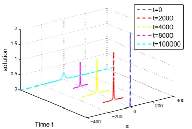
diffuses to zero, see Figure 7. If theM0 > MC the solution blows up as illustrated in Figure

−400 −200 0 200 400 0 0.5 1 1.5 2 x Time t solution t=0 t=2000 t=4000 t=8000 t=100000

Figure 7. M = 2π−0.1< Mc. Evolution of the density ρfor χ= 1.

−10 −5

0 5 10 0 10 20 30 40 50 60 x Time t solution t=0 t=3 t=6 t=9 t=12

−5 0

5 0

5 10 15

x 109

x Time t

solution

t=t*+33e−14

t=t*+51e−14

t=t*+57e−14

t=t*+58e−14

Figure 8. M = 2π+ 0.1> Mc. Evolution of the densityρforχ= 1, where t∗ = 16.818399684193.

Next we study the behavior of (17) for two initial densities corresponding to the sum of two Gaussians, i.e.

ρ1₀(x) = √600

2π−0.1

√

2π e

−600(x−2)2

2 + 2π√−0.5

2π e

−600(x+2)2

2

,

and

ρ2₀(x) =√600

2π+ 0.1

√

2π e

−600(x−2)2

2 + 2π√−0.5

2π e

−600(x+2)2

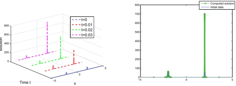
2

,

before getting closer to the center of mass, see Figure 10, again the final time does not correspond to the blow-up time.

−5

−2 0 2

5 0

50 100 150 200

x Time t

solution

t=0 t=0.3 t=1.5 t=1.8

−05 0 5

20 40 60 80 100 120 140 160 180 200 220

Computed solution Initial data

Figure 9. Evolution of the densityρforχ= 1 with initial datumρ0 =ρ10(x)

up to time t= 1.8.

−5

0

5 0

200 400 600 800

x Time t

solution

t=0 t=0.01 t=0.02 t=0.03

−50 0 5

100 200 300 400 500 600 700

800 Computed solution

Initial data

Figure 10. Evolution of the density ρ for χ = 1 with initial datum ρ0 = ρ2

0(x) up to timet = 0.03.

In caseM > Mc, it is conjectured that the first blow-up should happen by the formation

of a Dirac Delta with exactly the critical mass Mc= 2π. Moreover, a detailed asymptotic

However, we can now compare our computed diffeomorphism to the diffeomorphism representing the zeroth order term in the expansion studied by [36]. This expansion does not carry over directly to our modified KS system (17). Nevertheless, it is easy to check following [36] that the zeroth order term should be given by a properly scaled stationary state of the critical mass case. More precisely, the solution near the blow-up time should behave like

˜

ρ(t) = 2γ(t)

1/2

1 +γ(t)x2 with γ(t)'ρ(t,0) 2

in an interval of length 2L(t) centered at the point of blow-up withL(t)−1 'ρ(t,0) accord-ing to [36, 13]. In order to check this behavior, we try to avoid comparisons of the densities due to the numerical errors mentioned above and we concentrate in estimating the error between the diffeomorphisms Φ(t) and Ψ(t) representing ρ(t) and ˜ρ(t) respectively. The last one is computed by calculating the diffeomorphism representing the steady solution to the critical mass case 2(1 +x2₎−1 _{and then multiplying by the dilation factor γ(t)}−1/2_.

We take as initial data a Gaussian already very picked at the origin, i.e. (14) with

σ2 _{= 5×10}−6 _{and M = 2π + 0.1 for which we have numerical blow-up quite quickly.}

Let Ω = [−0.1,0.1] be the computational domain discretized into 1200 intervals of size ∆x = ₁₂₀₀0.2 . The discrete time steps are set to ∆t = 10−9_{. Then, we compute the}

blow-up time T = 3.328e −6 as the one for which our Newton’s iterations do not converge. Once the blow-up time is approximated, we compute the errors in Wasserstein distance betweenρ(t) and ˜ρ(t) on the interval (−L(t), L(t)) and we can compare the corresponding diffeomorphisms at the blow-up time. Figure (11)(a) shows the evolution in time of the

L2_{-difference between Φ(t) and Ψ(t) over the mass interval corresponding to (−L(t), L(t))}

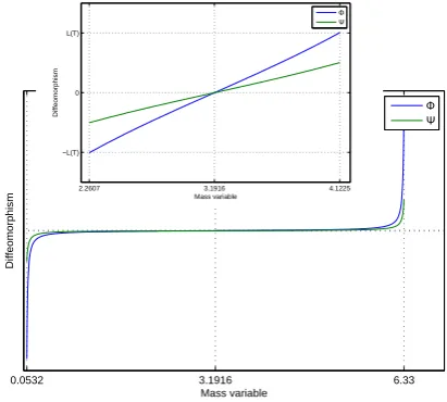
close to blow-up time. Figure (11)(b) shows the comparison between Φ(T) and Ψ(T) both over the mass interval of length 2π and the zoom over the mass interval corresponding to (−L(T), L(T)).

5.2. 2D simulations. Next we present several numerical simulations in 2D. Let Ω denote the unit circle, M=S

V∈VxV the computational mesh with vertexes xV, V ={1, . . . nV}

and N = S

V∈VΦ(xV) the transformed mesh. We choose the following parameters if not

stated otherwise:

• ∆t = 0.01

• nV = 1758 which corresponds to 3386 triangles of maximum size hmax = 0.05.

The initial datum is given by Gaussian centered around the origin

ρ0(x) =

1 2πσ2e

− 1

2σ2(x

2_+y2₎

+cwith σ = 0.3,

where c is chosen such that R

Ωρ0(x)dx = 1. In the pre-processing step we solve the heat

equation on the time interval t ∈ (0,2] using an implicit in time discretization and H1

-conforming elements of order 6. The solution is computed at ti = 0.002i, i = 1, . . . ,1000

and used for the computation of the initial diffeomorphism. The error bounds for the Newton schemes are set to 1 = 2 = 10−6, the regularization parameter ε in the

2.6 2.7 2.8 2.9 3 3.1 3.2 3.3 3.4 x 10−6 0

1 2 3 4 5 6x 10

−12

Time

L

2error

o

f

Φ

−

Ψ

(a)Evolution of the error indW betweenρ(t) and ˜ρ(t) near the blow-up time.

0.0532 3.1916 6.33

Mass variable

Diffeomorphism

Φ Ψ

2.2607 3.1916 4.1225

−L(T) 0 L(T)

Mass variable

Diffeomorphism

Φ Ψ

(b) Comparison of the diffeomorphisms Φ

and Ψ at the blow-up time T. Inset shows a zoom at the center of mass.

Figure 11. Comparison of the evolution of Φ(t) and Ψ(t).

5.2.1. Attraction potentials. First we consider an attraction potential of harmonic type

W(x) = 1₂|x|2_{. In the case of a purely attractive potential we expect the formation of a}

Delta Dirac at the center of the domain. Figure 12 illustrates the formation of the blow up. In the first picture we see the transformed mesh, where all triangles are moved towards the center of the domain. The second and third picture show the reconstructed density profile

ρ as well as the decay of the distance towards the Dirac Delta in time. The numerical simulations confirm the theoretical results, indicated by the red line of slope −1, at the beginning of the simulation. The bad match towards the end results most likely from the formation of the Delta Dirac and the inaccuracy caused by it.

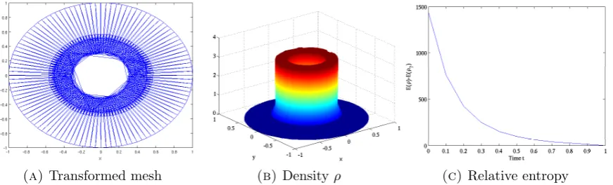
5.2.2. Attraction-repulsion potentials. Next consider the attraction-repulsion potential (16). In the casea= 4 andb = 2 the solution concentrates on a ring of radiusr= 1

2, see [39, 38].

The formation of the Delta Dirac ring is clearly visible in Figure 13. The first picture corresponds to the transformed initial mesh, the second and third show the reconstructed density and the decay of the relative entropy respectively. Note that we map the boundary of the computational domain onto itself, hence the boundary nodes do not move.

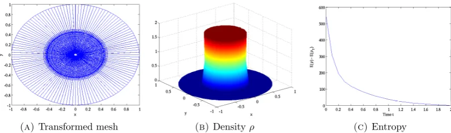
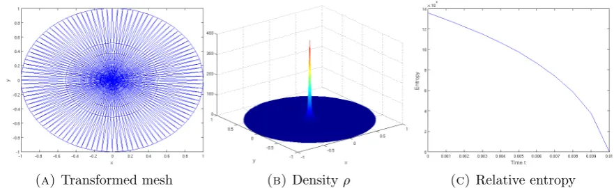
In the case of a logarithmic repulsion, that is a = 2 and b = 0 in (16) we expect the formation of a compactly supported steady state circle with radius r = 1₂. We see that the vertexes of the mesh concentrate in a circle of radius r = 1₂, except for the boundary nodes which are fixed, see Figure 14. Again the second and third plot correspond to the reconstructed density ρ at timet = 2 and the decay of the relative entropy functional.

(a) Transformed mesh (b) Densityρ (c)dW(ρ(t), δ0).

Figure 12. Simulation results in the case of a purely attractive potential

W = 1₂|x|2_.

(a) Transformed mesh (b)Densityρ (c) Relative entropy

Figure 13. Simulation results for an attractive-repulsive potential W =

1

4|x|

4₋1

2|x|

2_.

(a) Transformed mesh (b)Densityρ (c)Entropy

Figure 14. Simulation result for an attractive-repulsive potential W =

1

2|x|

the form V(x) = −α

βln(|x|). This model has been proposed as a way to find the spatial

(a) Transformed mesh (b) Densityρ (c)Relative entropy

Figure 15. Simulation results for an attractive-repulsive potential W =

1

2|x|

2_{−ln(|x|) and an additional potential V =} 1

4ln(|x|).

shape of the milling profiles in microscopic models for the dynamics of bird flocks [18]. We obtain this steady state also in the numerical simulations, see Figure 15. The inner and outer radius of this mill depend on the parametersα and β and are given

Ri =

r_α

β and Ro =

r α

β +

1 2π.

see [23]. The transformed mesh clearly shows the formation of the steady state annulus with α = 1 and β = 4. Note that the ’vacuum formation’ at the center distorts the mesh at the center. Note that the distortion of the triangles in Figure 15 does not affect the performance of the numerical method itself, since all computations are done using the original mesh on the reference domain ˜Ω. It only affects the reconstruction of the final densityρ, where we observe numerical instabilities close to the support of the steady state annulus. Therefore we choose to solve a regularized version of (5).

If we start with a not radially symmetric initial datum of the form

ρ0(x) = 1

4π0.252e

− 1

20.252((x−0.15)

2_(y−0.25)2₎

+ 1

4π0.22e

− 1

20.22((x+0.3)

2_+(y+0.4)2₎

and again consider a potential of the form (16) witha= 2, b= 0, we observe the formation of an off-centered compactly supported bump, see Figure 16.

5.2.3. The Keller-Segel model. In our final example we consider the modified KS model (17) with an initial Gaussian of mass one and χ = 1.1× 8π. The time steps are set to ∆t = 5×10−3 _{and we observe the fast formation of a Delta Dirac at the center of}

(a) Transformed mesh (b)Densityρ (c) Relative entropy

Figure 16. Simulation results for an attractive-repulsive potential W =

1

2|x|

2_{−ln(|x|) in case of a not radially symmetric initial datum.}

(a) Transformed mesh (b) Densityρ (c)Relative entropy

Figure 17. Simulation results for KS model with initial M = 1 and χ = 1.1×8π.

6. _Conclusion

The 2D algorithm involves several pre- and post-processing steps, which present addi-tional challenges with respect to numerical accuracy and computaaddi-tional complexity. The proposed finite element discretization allows to consider more general domains and better resolve features of radially symmetric solutions, which often arise in aggregation equations. However the computational complexity of the preprocessing step as well as the solver itself remains a key limitation of the solver, which we plan to address in a future work.

Acknowledgments

JAC was partially supported by the Royal Society via a Wolfson Research Merit Award. HR and MTW acknowledge financial support from the Austrian Academy of Sciences ¨OAW via the New Frontiers Group NSP-001. The authors would like to thank the King Abdullah University of Science and Technology for its hospitality and partial support while preparing the manuscript.

References

References

[1] G. Albi, D. Balagu´e, J. A. Carrillo, and J. von Brecht. Stability analysis of flock and mill rings for second order models in swarming.SIAM J. Appl. Math., 74(3):794–818, 2014.

[2] L. Ambrosio, N. Gigli, and G. Savar´e.Gradient flows. Springer, 2005.

[3] Luigi Ambrosio, Stefano Lisini, and Giuseppe Savar´e. Stability of flows associated to gradient vector fields and convergence of iterated transport maps.manuscripta mathematica, 121(1):1–50, 2006. [4] Albert Avinyo, Joan Sola-Morales, and Marta Valencia. On maps with given Jacobians involving the

heat equation.Zeitschrift f¨ur angewandte Mathematik und Physik ZAMP, 54(6):919–936, 2003. [5] D. Balagu´e, J. A. Carrillo, T. Laurent, and G. Raoul. Dimensionality of local minimizers of the

interaction energy.Arch. Ration. Mech. Anal., 209(3):1055–1088, 2013.

[6] D. Balagu´e, J. A. Carrillo, T. Laurent, and G. Raoul. Nonlocal interactions by repulsive-attractive potentials: radial ins/stability.Phys. D, 260:5–25, 2013.

[7] Jean-David Benamou, Guillaume Carlier, Quentin M´erigot, and Edouard Oudet. Discretization of functionals involving the Monge–Amp`ere operator.Numerische Mathematik, pages 1–26, 2014. [8] A. J. Bernoff and C. M. Topaz. A primer of swarm equilibria.SIAM J. Appl. Dyn. Syst., 10(1):212–250,

2011.

[9] Andrea L. Bertozzi, Jos´e A. Carrillo, and Thomas Laurent. Blow-up in multidimensional aggregation equations with mildly singular interaction kernels.Nonlinearity, 22(3):683–710, 2009.

[10] Adrien Blanchet, Vincent Calvez, and Jos´e A Carrillo. Convergence of the mass-transport steepest descent scheme for the subcritical Patlak-Keller-Segel model.SIAM Journal on Numerical Analysis, 46(2):691–721, 2008.

[11] Adrien Blanchet, Jos´e A. Carrillo, and Philippe Lauren¸cot. Critical mass for a Patlak-Keller-Segel model with degenerate diffusion in higher dimensions. Calc. Var. Partial Differential Equations, 35(2):133–168, 2009.

[12] Adrien Blanchet, Jos´e A Carrillo, and Nader Masmoudi. Infinite time aggregation for the critical Patlak-Keller-Segel model in _R2_{. Communications on Pure and Applied Mathematics, 61(10):1449–}

1481, 2008.

[14] CJ Budd, GJ Collins, WZ Huang, and RD Russell. Self–similar numerical solutions of the porous– medium equation using moving mesh methods.Phil. Trans. R. Soc. A: Mathematical, Physical and

Engineering Sciences, 357(1754):1047–1077, 1999.

[15] Vincent Calvez, Benoˆıt Perthame, and Mohsen Sharifi Tabar. Modified Keller-Segel system and critical mass for the log interaction kernel.Contemp. Math., 429:45–62, 2007.

[16] J. A. Carrillo, M. Di Francesco, A. Figalli, T. Laurent, and D. Slepcev. Global-in-time weak measure solutions and finite-time aggregation for nonlocal interaction equations.Duke Mathematical Journal, 156(2):229–271, FEB 1 2011.

[17] J A Carrillo, Marco Di Francesco, and Giuseppe Toscani. Strict contractivity of the 2- Wasserstein dis-tance for the porous medium equation by mass-centering.Proceedings of the American Mathematical

Society, 135(2):353–363, 2007.

[18] J. A. Carrillo, M. R. D’Orsogna, and V. Panferov. Double milling in self-propelled swarms from kinetic theory.Kinet. Relat. Models, 2(2):363–378, 2009.

[19] J. A. Carrillo, M. Fornasier, G. Toscani, and F. Vecil. Particle, kinetic, and hydrodynamic models of swarming. InMathematical modeling of collective behavior in socio-economic and life sciences, Model. Simul. Sci. Eng. Technol., pages 297–336. Birkh¨auser Boston, Inc., Boston, MA, 2010.

[20] J. A. Carrillo, Y. Huang, and S. Martin. Explicit flock solutions for Quasi-Morse potentials.European

J. Appl. Math., 25(5):553–578, 2014.

[21] J A Carrillo, Y Huang, F S Patacchini, and G Wolansky. Numerical study of a particle method for gradient flows.arXiv preprint arXiv:1512.03029, 2015.

[22] J. A. Carrillo, S. Martin, and V. Panferov. A new interaction potential for swarming models. Phys. D, 260:112–126, 2013.

[23] Jos´e A Carrillo, Alina Chertock, and Yanghong Huang. A finite-volume method for nonlinear nonlocal equations with a gradient flow structure.Communications in Computational Physics, 17(01):233–258, 2015.

[24] Jos´e A Carrillo, Lucas CF Ferreira, and Juliana C Precioso. A mass-transportation approach to a one dimensional fluid mechanics model with nonlocal velocity.Advances in Mathematics, 231(1):306–327, 2012.

[25] Jos´e A Carrillo, Robert J McCann, C´edric Villani, et al. Kinetic equilibration rates for granular media and related equations: entropy dissipation and mass transportation estimates. Revista Matematica

Iberoamericana, 19(3):971–1018, 2003.

[26] Jos´e A Carrillo and J Salvador Moll. Numerical simulation of diffusive and aggregation phenomena in nonlinear continuity equations by evolving diffeomorphisms.SIAM Journal on Scientific Computing, 31(6):4305, 2009.

[27] M. R. D’Orsogna, Y.-L. Chuang, A. L. Bertozzi, and L. S. Chayes. Self-propelled particles with soft-core interactions: patterns, stability, and collapse.Physical review letters, 96(10):104302, 2006. [28] Bertram D¨uring, Daniel Matthes, and Josipa Pina Miliˇsic. A gradient flow scheme for nonlinear fourth

order equations.Discrete Contin. Dyn. Syst. Ser. B, 14(3):935–959, 2010.

[29] L. Evans, O. Savin, and W. Gangbo. Diffeomorphisms and nonlinear heat flows. SIAM Journal on

Mathematical Analysis, 37(3):737–751, 2005.

[30] Klemens Fellner and Ga¨el Raoul. Stable stationary states of non-local interaction equations.

Mathe-matical Models and Methods in Applied Sciences, 20(12):2267–2291, 2010.

[31] Klemens Fellner and Ga¨el Raoul. Stability of stationary states of non-local equations with singular interaction potentials.Mathematical and Computer Modelling, 53(7):1436–1450, 2011.

[32] Michael T Gastner and Mark EJ Newman. Diffusion-based method for producing density-equalizing maps.PNAS, 101(20):7499–7504, 2004.

[33] Laurent Gosse and Giuseppe Toscani. Identification of asymptotic decay to self-similarity for one-dimensional filtration equations.SIAM Journal on Numerical Analysis, 43(6):2590–2606, 2006. [34] Laurent Gosse and Giuseppe Toscani. Lagrangian numerical approximations to one-dimensional

[35] S. Haker and A. Tannenbaum. Optimal mass transport and image registration. In Variational and

Level Set Methods in Computer Vision, 2001. Proceedings. IEEE Workshop on, pages 29 –36, 2001.

[36] Miguel A. Herrero and Juan J. L. Vel´azquez. Singularity patterns in a chemotaxis model.Math. Ann., 306(3):583–623, 1996.

[37] Darryl D. Holm and Vakhtang Putkaradze. Aggregation of finite-size particles with variable mobility.

Phys. Rev. Lett., 95:226106, Nov 2005.

[38] Yanghong Huang and Andrea Bertozzi. Asymptotics of blowup solutions for the aggregation equation.

Discrete Contin. Dyn. Syst. Ser. B, 17(4):1309–1331, 2012.

[39] Yanghong Huang and Andrea L. Bertozzi. Self-similar blowup solutions to an aggregation equation

inRn_{.SIAM J. Appl. Math., 70(7):2582–2603, 2010.}

[40] Richard Jordan, David Kinderlehrer, and Felix Otto. The variational formulation of the Fokker–Planck equation.SIAM Journal on Mathematical Analysis, 29(1):1–17, 1998.

[41] Oliver Junge, Daniel Matthes, and Horst Osberger. A fully discrete variational scheme for solving nonlinear Fokker-Planck equations in higher space dimensions.arXiv preprint arXiv:1509.07721, 2015. [42] T. Kolokolnikov, J. A. Carrillo, A. Bertozzi, R. Fetecau, and M. Lewis. Emergent behaviour in

multi-particle systems with non-local interactions [Editorial].Phys. D, 260:1–4, 2013.

[43] Theodore Kolokolnikov, Hui Sun, David Uminsky, and Andrea L. Bertozzi. Stability of ring patterns arising from two-dimensional particle interactions.Phys. Rev. E, 84:015203, Jul 2011.

[44] A. J. Leverentz, C. M. Topaz, and A. J. Bernoff. Asymptotic dynamics of attractive-repulsive swarms.

SIAM J. Appl. Dyn. Syst., 8(3):880–908, 2009.

[45] Daniel Matthes and Horst Osberger. Convergence of a variational Lagrangian scheme for a nonlinear drift diffusion equation. ESAIM: Mathematical Modelling and Numerical Analysis, 48(03):697–726, 2014.

[46] A. Mogilner and L. Edelstein-Keshet. A non-local model for a swarm.Journal of Mathematical Biology, 38(6):534–570, 1999.

[47] J¨urgen Moser. On the volume elements on a manifold. Transactions of the American Mathematical

Society, pages 286–294, 1965.

[48] Felix Otto. The geometry of dissipative evolution equations: the porous medium equation. Comm.

Partial Differential Equations, 26(1-2):101–174, 2001.

[49] E. B. Saff and V. Totik.Logarithmic potentials with external fields. Grundlehren der mathematischen Wissenschaften. Springer, Berlin, New York.

[50] C. M. Topaz and A. L. Bertozzi. Swarming patterns in a two-dimensional kinematic model for bio-logical groups.SIAM J. Appl. Math., 65(1):152–174, 2004.

[51] C. M. Topaz, A. L. Bertozzi, and M. A. Lewis. A nonlocal continuum model for biological aggregation.

Bull. Math. Biol., 68(7):1601–1623, 2006.

[52] Giuseppe Toscani. One-dimensional kinetic models of granular flows. M2AN Math. Model. Numer.

Anal., 34(6):1277–1291, 2000.

[53] Juan Luis V´azquez. Smoothing and decay estimates for nonlinear parabolic equations of porous medium type.Oxford Lecture Notes in Maths and its Applications, 33, 2006.

[54] J. J. L. Vel´azquez. Point dynamics in a singular limit of the Keller-Segel model. I. Motion of the concentration regions.SIAM J. Appl. Math., 64(4):1198–1223, 2004.

[55] C´edric Villani. Topics in Optimal Transportation, volume 58 of Graduate Studies in Mathematics. American Mathematical Society, Providence, RI, 2003.

[56] Michael Westdickenberg and Jon Wilkening. Variational particle schemes for the porous medium equa-tion and for the system of isentropic Euler equaequa-tions.ESAIM: Mathematical Modelling and Numerical

Analysis, 44(01):133–166, 2010.

[57] Y. Yao and A. L. Bertozzi. Blow-up dynamics for the aggregation equation with degenerate diffusion.