Explosive condensation in symmetric mass transport models

(1)

University of Warwick institutional repository:

http://go.warwick.ac.uk/wrap

A Thesis Submitted for the Degree of PhD at the University of Warwick

http://go.warwick.ac.uk/wrap/77689

This thesis is made available online and is protected by original copyright.

Please scroll down to view the document itself.

(2)

Explosive condensation in symmetric mass transport models

by

Yu-Xi Chau

Thesis

Submitted to the University of Warwick

for the degree of

Doctor of Philosophy

Centre for Complexity Science and Mathematics Institute

(3)

Acknowledgments

Firstly, I would like to thank my supervisor Stefan Grosskinsky for his continuous support,

gratitude and patience throughout the duration of my study. He has always been a great

teacher, and his intellect, enthusiasm, warmth and humour will be missed. His door is

always open, and I really enjoyed many of our conversations.

I would also like thank my second supervisor Colm Connaughton, who has always

been encouraging, welcoming and friendly. My supervisors make my time in the

Com-plexity DTC very pleasurable and memorable. I owe a lot to the ComCom-plexity DTC, for

their understanding and help throughout my PhD studies, especially Prof. Robert MacKay

and Prof. Robin Ball. And to Complexity DTC administrators Monica de Lucena, Phil

Richardson, Jen Bowskill, Heather Robson and Deborah Walker for their assistance and

resourcefulness. I am also very grateful for my fellow students in the DTC, having always

been supportive at an intellectual level. I would like to thank especially Anas Rana, Dominic

Kerr, Anthony Woolcock, Mike Maitland and Arran Tamsett for the countless discussions

we have had over the years.

My time in graduate school has been a time of great emotional and spiritual

jour-ney, and I would thank all my friends for their support outside my studies. Especially my

mentors Elaine Tang and Chernise Neo for their invitations and challenges. Martine Barons

and Phil Richardson for their spiritual guidance inside the Complexity DTC. Also members

of the Westwood Church, especially Peter Findley, Pinmei Huang, Caroline Howarth and

Oliver Howarth, for the community, conversations and good food.

Finally, I would like to thank my family, especially my parents and brother for their

constant support. Also, I am forever in debt to Helen Miu for her patience and looking after

(7)

Declarations

This work has been composed by myself and has not been submitted to other degree or

professional qualification.

• The novel and original contributions of this thesis are presented in Chapters 4 to 6.

(8)

Abstract

Condensation is an emergent phenomenon in complex systems that is observed in both physical and social sciences, from granular polydisperse spheres to macroeconomic studies. The critical behaviour of condensation in such systems is of continual interest in research. In this thesis we study this in the context of interacting particle systems, in particular the recently introduced explosive condensation process.

We firstly provide a review of the mathematical foundations of interacting particle systems from the aspects of Markov processes. This includes the formulation of factorised hop rates, stationary product measures, the equivalence of ensembles and how these proper-ties are related to condensation. Subsequently, we give a review of key interacting particle systems of interest, namely the zero-range process, inclusion process and the explosive condensation process. We then introduce two models that have similar stationary weights scaling as the explosive condensation process and include them in our study in the thermo-dynamic limit.

The density and the maximum site occupation are derived under the stationary dis-tribution, and from this we are able to identify the choice of parameters that could lead to a phase transition. Exact results for these models using the generator are difficult to ob-tain. For the main results of this study, we therefore analyse the formation of condensate using a heuristic approach. The microscopic interactions leading to the formation of an explosive condensate are structurally studied, and this leads to a comprehensive model with a timescale analysis. The time to condensation is shown to vanish as the thermodynamic limit is reached, depending on the choice of parameter values.

(9)

Notation

Below are some important notations used throughout the thesis, listed in chronological

order of introduction:

Λ Countable lattice (p. 5)

X_Λ State spaceX_Λ=_NΛ(p. 5) L Size of countable lattice (p. 5)

η=(ηx)x∈ΛL Full configuration (p. 5)

ηx (p. 5)

N Total number of particles in system, i.e.P

x∈Ληx= N(p. 5) c(η, η0) Transition rate from configurationηtoη0(p. 5)

ηxy _{New configuration after a particle is moved from site}_x_→_y_in_η_{(p. 5)}

L Generator (p. 6)

f(η) An observable over configurationη(p. 6)

R Real numbers (p. 6)

E Expected value of (p. 6)

x,y Typical lattice sites (p. 6)

p(x,y) Adjacency matrix (p. 7)

u(n),v(n) Factorised hop rates of transition rate (p. 7)

φ System fugacity (p. 8)

(10)

W Stationary weights (p. 8)

R(φ) Average number of particles per site (p. 8)

σ2 _{Second moment of the system (p. 9)}

k∞ The∞denoteskin long relaxation times, ort→ ∞(p. 9)

ρc Critical density (p. 10)

d Diffusive parameter (p. 17)

TSS Time for the system to reach stationarity (p. 20)

ηmax Occupancy of the highest occupied site in the system (p. 28)

G(L,Sc) Denoting the Erd˝os-R˝enyi graph, whereSc =(1/LPx,y∈Λp(x,y) (p. 34) c(ηx, ηy) Another form for transition rates, which depends on the local configuration

ηx, ηy(p. 46)

mc Critical occupancy number (p. 49)

τstep Time for an entire cluster to move one lattice space (p. 53)

v(m)=1/hτ_stepi Average velocity for an entire cluster to move one lattice space (p. 54)

∆m The transfer of mass from the smaller to the larger cluster when two clusters collide (p. 58)

p_split Probability of a cluster to spontaneously split up into two separate clusters in opposed to moving to a neighbouring site. (p. 87)

rsplit=v(m)psplit The rate of a split (p. 88)

Nbr Total number of clusters breaking up in the timescale when a system reaches stationarity (p. 89)

(11)

Below are suffixes used throughout the thesis, that is related to either the graph, model or a

process:

Wa relating to the model with rates (3.2)

mod relating to the “modified” model with rates (3.3)

gen relating to the “generalised” model with rates (6.1)

sym relating to cases on a symmetric graph

asym relating to cases on a totally asymmetric graph

Nu relating to the cluster nucleation phase

(12)

Chapter 1

Introduction

Statistical mechanics provides a qualitative connection between macroscopic physical laws

and microscopic rules of interactions for large physical systems using statistical methods. The origin of statistical mechanics is in thermodynamics, where a class of continuous

phys-ical measures can be explained by atomic interactions using probabilistic arguments.

Ex-tremely large system sizes of the order of 1023 particles lead to very small fluctuations around the typical behaviour, which can be derived in a thermodynamic scaling limit. Since

its early development, statistical mechanics has become a convenient mathematical tool that

is used for systems with a large number of interacting components, not constrained to phys-ical models only. Examples include traffic flow, economics, crowd dynamics, etc. In theory,

a microscopic description of such systems is deterministic, but impractical due the number

of degrees of freedom. Due to the robustness of the system on a macroscopic scale with respect to noise, it is often sufficient to approximate the microscopic behaviour in terms of

randomness with a postulated probability distribution.

With a probabilistic description, the system is characterised by the expected values of certain observables, which correspond to the microscopic state space measurable

func-tions. For systems in equilibrium in the thermodynamic limit, where the size is very large,

these observables can be calculated by a small number of macroscopic system parameters, such as density, temperature and pressure. One area that is particularly studied is the ability

of the system to exhibit phase transitions, where qualitative changes in the typical behaviour

of observables occur when some parameters are varied. In such cases, abrupt transitions of some macroscopic observables can be observed.

For systems with many identical components which are in equilibrium with the sur-roundings, the stationary long-time behaviour is described by an energy function or the

Hamiltonian. In this scenario the typical value of macroscopic observables is given by

(13)

exten-sively studied in the physical literature, since the work of Boltzmann, and there is now a

well developed mathematical theory [2, 3]. There is also a well developed mathematical

understanding of phase transitions in such systems in terms of Gibbs measures [4].

Although there are few general physical laws that apply to non-equilibrium systems,

insights can be drawn by studying interacting particle systems. They consists of particles

on a lattice, where the exchange of particles between sites is given by rates that depend on the system configuration. Mathematically they can be regarded as continuous-time Markov

process on a discrete state space. The rules of interactions can be altered to represent any

microscopic phenomena of interest. These models have been popular in various fields, such as physics, chemistry, biology, social sciences, etc. The underlying process may be defined

in terms of discrete particles on some lattice, for example cellular growth of cells on a

2-dimensional surface. Naturally, a phenomenological description is used to describe these interacting particle models, in the sense that they serve as an approximation to their true

underlying microscopic dynamics. Therefore, interacting particle systems may be regarded

as mesoscopic models. These models are popular in physics and mathematics because of their broad application and rich non-trivial characteristics despite their simplistic set-up.

A particularly well studied model encompassing these characteristics is the zero-range process, which is used to explain physical systems such as polydisperse spheres,

quantum gravity and traffic jams [5]. There is no restriction on the number of particles

on each site, and the transition rate is dependent on the occupancy of the departure site only. Despite its seemingly simple set-up, it displays non-trivial behaviour even in a

one-dimensional geometry. A natural progression from the zero-range model is models with

transition rates that depend on the occupancies of both the departure and receiving sites. These give rise to increasing research interest for new models such as the inclusion process,

and more recently, the explosive condensation process [6]. Condensation occurs when a

positive fraction of the mass of the system is concentrated on one lattice site. This can occur for both inhomogeneous and homogeneous graphs. We are particularly interested in

the homogeneous cases of explosive condensation in this study, and we focus on the cases

where the overall mass of the system is a conserved quantity. Explosive condensation is a phenomena observed in some condensation models, where the time to reach the condensate

goes to zero as the system sizeLdiverges. This is seemingly counter-intuitive as it implies that stationarity is reached instantly if the system size is infinitely large.

To clarify the ideas mentioned above, we describe a social science analogy of phase

transition in condensation as an example, with one that concerns the trading of wealth in

an agrarian society. Land is the primary source of wealth in agricultural societies, and is usually conserved. Therefore wealth is largely conserved over long timescales in ancient

(14)

where interactions are biased under the frameworks of information economics. This rule of

exchange is embedded in a global redistribution of wealth in the form of poll tax. A defining

feature is when systems transit from a relatively equal distribution to a phase of great wealth disparities. It is observed as a historical phenomenon that great wealth disparity is always

the stationary state for relatively prosperous closed societies. Primitive societies are known

to exist for centuries with a largely intact “fluid state” of wealth. At some critical density, when overall wealth in the society increases, huge wealth disparities would be observed.

The Matthew principle states that the greater wealth in the system, the faster the speed of

wealth condensation [7, 8]. In this situation, wealth is divided between a ubiquitous fluid state and a condensate.

In Chapter 2 we summarise the results from existing literature on interacting particle

systems, introducing the concepts of generators and stationary product measures. Several models are reviewed to discuss recent areas of research interest. Models that are similar to

the explosive condensation model are introduced in Chapter 3 and we attempt to retrieve

meaningful results from the generator. In Chapter 4, we study the dynamics of models introduced in the previous Chapter heuristically in the thermodynamic limit. This gives

rise to a comprehensive explanation of the formation of the explosive condensate, where distinctive stages of cluster interactions are studied. The nucleation and coarsening driven

model in Chapter 4 also leads to a simpler explanation for previous studies [6]. In Chapter

5, we discuss numerical methods for this study. An algorithm that improves numerical efficiency yet preserving stochastic properties is introduced. Two variants of the model

studied in Chapter 4 are introduced in Chapter 6, which extend this study to inhomogeneous

(15)

Chapter 2

Interacting Particle Systems

2.1 Introduction

Interacting particle systems (IPS) were originally studied as a branch of probability theory [9, 10], but have since grown and developed rapidly, establishing connections with

applica-tions in physics, biology and social sciences [5]. The original motivation for IPS came from

statistical mechanics. The objective was to describe and analyse stochastic models for the temporal evolution of systems with classical Gibbs states as their equilibrium measures [11]

[12]. In particular, it was hoped that the study of IPS would lead to a better understanding

of the phenomenon of phase transitions.

Through the works of Liggett [13] and Dobrushin [11], foundations of IPS were

studied in the early 1970s. The introduction of IPS is a natural extension of the

estab-lished theory of Markov processes. A typical set-up of IPS consists of having a finite or infinite number of particles on a lattice, with some interaction rules outlining how particles

are transferred between sites. The interaction between particles implies that the system is

more complex than simple independent particles, and has to be described on a very high dimensional state space.

Interacting particle systems have since developed and became an independent study area that connects the mathematical description of different physical systems; such as neural

networks [14], tumour growth [15], spread of infection [16], wealth distribution models [17], traffic jams [18, 19] population ecology [20], behavioural systems [21, 22] and many others. This involves using different types of transition rates on different graphs. A review

of models relevant to this thesis can be found in Sec. 2.3. Even though the set up is generally

simple, a rich complex behaviour can be seen already in one-dimensional systems.

In this chapter, the ideas for the foundations of IPS are described and a brief

(16)

provided in this chapter in Sec. 2.2 will be used throughout this thesis. A standard

for-mulation of an IPS using the generator, definition of transition rates as factorized hop rates

are introduced in Sec. 2.2.1 - 2.2.3. Selected models that have attracted recent research attention are summarised in Sec. 2.3. These include the classic zero-range process and the

more recently introduced inclusion process and explosive condensation process.

2.2 Definitions

A detailed description of the notation and definitions used throughout this study are

pro-vided in this section. The notation used in this work are largely taken from Chleboun and Grosskinsky [23], Grosskinsky, Sch¨utz and Spohn [24] and also more distantly from Liggett

[13].

Essentially, interacting particle systems are a class of continuous-time Markov pro-cesses on discrete state spaces with states given by particle configurations on a lattice or

general graph. Systems with both infinite and finite lattice sizes are possible, but this study

focuses on closed finite systems and their scaling behaviour. The dynamics of these pro-cesses are typically characterized by infinitesimal transition rates at which transitions

be-tween states occur.

The state space X_Λ = NΛ contains all possible particle configurations, where Λ denotes a countable lattice that can be finite or infinitely large. As this study focuses on

finite systems, usuallyΛL = {1,2, ...,L}is finite andLdenotes its finite size. In this study,

we restrict the lattice to being one-dimensional. The configuration of the system is given by

η= (ηx)x∈Λ, such thatηx ∈Ndenotes the number of particles at site x. The total number of particles on a finite system is thereforeN=P

x∈Ληx.

We focus on local jumps, where a single particle changes location, and denote by

ηxy_{the resulting configuration after a jump from}_x_to_y_∈_Λ_{, where}

ηxy

z :=ηz−δz,x+δz,y, (2.1)

andδ is the Kronecker delta function and all x,y,z ∈ X. Site x can be regarded as the departure site and siteyis the receiving site. Note that such transitions only occur if sitex has non-zero mass prior to an interaction.

The interaction of the particle system is characterized by transition rates c(η, η0) for the transition from one configuration to another. These infinitesimal transition rates are

used to define the generator of the process (see Sec. 2.2.1), which uniquely characterises the

time evolution using Markov semigroups and the Hille-Yosida theorem. In the following we give a short account of these tools, and for a rigorous mathematical formulation of these

(17)

2.2.1 Generator

The transition rate of a system is given byc(η, η0)≥0 which, for allη, η0∈X, describes the rate at which the system changes from the current stateηto a new stateη0. The generator

Loperating on a general observable f :X_Λ→_Ris defined as

Lf(η)= X

η0_∈_X

c(η, η0)(f(η0)− f(η)) , (2.2)

with the conventionc(η, η) = 0 for all η ∈ X. The observable f(η) can be any physical property derived from the configuration, such as the average number of particles, the second moment of the configuration, etc. The dynamics on a finite latticeΛLare defined by the

generator, in the sense that

d

dtE[f(η)]=E[Lf(η)]. (2.3)

This becomes a very convenient tool for studying Interacting Particle Systems, where the time evolution of any observable of interest can be expressed as a differential

equation. This form is equivalent to the description of the master equation for the IPS.

Denoting the probability distribution onX_Λat timetby p_t[η], the master equation is given by

d

dtpt[η]= X

η∈X

(p_t[η]c(η, η0)− p_t[η0]c(η0, η)) , (2.4)

which displays gain and loss terms on the right-hand side and follows from Eq. (2.3) by

using the indicator function f =δη. However, it is convenient to use the generator because its set up allows us to write down a time-dependent relationship for any designated set of

observables, rather than the general distribution of the configuration. Note that the process

is derived from the generator by constructing a Markov semigroup and closing it using the Hille-Yosida theorem, for which the rigorous mathematical formulation can be found in

Chapters I and II of [10].

2.2.2 Factorized hop rate

From this point onwards, we deviate from the general IPS set-up and focus on a set of

formulation of the model that has attracted great research attention for the past years (see e.g. [23] and references therein). For pairwise interactions, the most common form for

interacting particle systems is when the rates of interaction are dependent on the mass of

(18)

c(η, ηxy)=u(ηx)v(ηy)p(x,y) , (2.5)

whereu(ηx) andv(ηy) represent the independent contributions from the occupancies of the

departure and receiving sites, respectively. p(x,y) is the adjacency matrix depicting the connectivity on the graphΛ. The factorized hop rates must satisfy

u(n)=0 if and only ifn=0,

v(n)>0 for alln≥0 . (2.6)

The reason why factorized hop rates attracted so much interest in interacting particle systems research is because of its simplicity and the rich behaviour it demonstrates. It

has also been established that systems with factorized hop rates have stationary product

measures, as outlined in the following sections.

The adjacency matrix is given by the transition rates of a single random walker on Λwhere p(x,y) ≥ 0 and p(x,x) = 0. Note that only irreducible cases are studied to avoid hidden conservation laws in this thesis. Throughout this thesis, we focus on two specific cases of the adjacency matrix in the literature, namely the totally asymmetric graph and the

symmetric graph in one dimension. For the totally asymmetric graph,

p(x,y)=

      

1 , fory= x+1

0 , otherwise , (2.7)

and for the nearest neighbour symmetric graph,

p(x,y)=

      

1 , for|x−y|=1

0 , otherwise . (2.8)

The generator in (2.2) is now rewritten as

Lf(η)= X

x,y∈Λ

p(x,y)u(ηx)v(ηy)(f(ηxy)− f(η)) , (2.9)

which is its full form. Under this specific framework of interacting particle systems listed above, several examples are reviewed later in this chapter and they are

• zero-range process (ZRP):u(n) arbitrary,v(n) = 1 (see Sec. 2.3.1, with a brief dis-cussion for its mapping onto the exclusion process),

(19)

• explosive condensation process (ECP):u(n)=v(n)−v(0), wherev(n)=(d+n)γ, and d, γ >0 (see Sec. 2.3.3).

Note that the interaction of particles are characterized by the above generator. Fo-cusing on the scaling properties of finite systems in the thermodynamic limit,Nis the total number of particles in this system, when forL → ∞andN → ∞, the densityρ = N/Lis fixed.

2.2.3 Stationary Product Measure and Condensation

A stationary distribution for the process is a probability distribution which is invariant under the dynamics, where the distribution of the measure at timetconverges to whent → ∞. A measureνon Xis stationary if and only ifν(Lf) = 0 for all observables, for a proof of this property, see Chapter 2 in [10]. If a system has translation invariant stationary product measure, it will be written as

νL

φ[η]=

Y

x∈ΛL

νφ(ηx) , (2.10)

defined by product densities w.r.t. the product counting measure dη on X_Λ, where the fugacityφ≥0 is a parameter that controls the density of the system and will be made clear with the derivation below. The marginals therefore have the form

νφ(n)= 1

z(φ)W(n)φ

n

. (2.11)

It should be noted in the totally asymmetric and symmetric cases, p(x,y) is translation in-variant. Since it is assumed that p(x,y) is irreducible, on finite lattices Λ, this is in fact unique up to normalization and strictly positive. The composition of the weights is

deter-mined by the independent contributions of the factorized hop rates.W(n) is written as

W(n)=

n Y

k=1

v(k−1)

u(k) , (2.12)

which contains the factorised form of the rates as illustrated in (2.5). The normalization

z(φ) is a partition function and has the form

z(φ)= ∞

X

n=0

W(n)φn. (2.13)

(20)

R(φ)=hηxiφ=

∞

X

k=0

kνφ[k]= 1 z(φ)

∞

X

n=0

nW(n)(λφ)n, (2.14)

which is a strictly monotonically increasing function withR(0)=0. For systems with con-served mass, the measures are therefore indexed by a fugacity parameterφ≥0 controlling the average number of particles per site.

Moment Generating Function

Since the partition functionz(φ) is a moment generating function, (2.14) can also be written as

∂logz(φ)

∂φ =

1 z(φ)

∞

X

n=0

λn

nφn−1W(n) . (2.15)

From (2.15), (2.14) is written as

R(φ)=φ ∂

∂φlogz(φ) . (2.16)

Throughout this study, the second moment is measured as a physical quantity and it can be

derived in a similar fashion. This is further explained in Sec. 3.3. The second moment at

the steady state ast→ ∞is given by

hσ2_∞(φ)i= 1

z(φ) ∞

X

n=0

n2W(n)(λφ)n, (2.17)

and similarly the second moment depicted in (2.17) can be written conveniently as the

moment generator form

hσ2_∞i=φ∂φφ∂φlogz(φ) . (2.18)

Although it may not be clear why we want to obtain a prediction of the second moment, this

will become an important property in studying the dynamics of the Explosive Condensation

Process, which is the focus of this thesis. The convenience of being able to determine the second moment of the stationary distribution allows us to estimate important scaling

properties.

Radius of Convergence

(21)

DΛ_φ ={φ≥0 :z(φ)<∞for allx∈Λ} (2.19) the domain of definition. Sincez(φ) is a power series inφ, the domain is actually of the form

DΛ_φ =[0, φ) or [0, φc] , (2.20)

where

φc =

λlim

n→∞supW(n) 1/n−1

. (2.21)

is the radius of convergence ofz(φ).

The Particle density ρ has the range [0, ρc) or [0, ρc], with ρ(0) = 0 and ρc =

limφ%φcR(φ) the critical density. φ → R(φ) is strictly increasing. The inverse of R is denoted byφ(ρ) on the range [0, ρc). Ifφc = ∞, thenρc = ∞. Whereas ifφc < ∞, both

ρc = ∞andρc < ∞are possible. In the second case, z(φc) < ∞andνφc is a well defined probability measure withhηxiνφc =ρc. Soφ(ρ) is given by

φ(ρ)=

      

inverse ofR(φ) , forρ < ρc

φc, forρ≥ρc

. (2.22)

System with Conserved Mass

We are interested in understanding how condensation occurs in systems with fixed size and mass. For a system with system sizeLand total massN≥0, the new state space will be

XL,N =       

η∈X_Λ X

x∈Λ

ηx =N        , (2.23)

on which the system is a finite state irreducible Markov process. The ergodicity of the

pro-cess means there exists a unique stationary measure that belongs to the canonical ensemble. This stationary measure is written as

πL

N[η] :=νφ       η X

x∈Λ

ηx= N       = 1 z(L,N)

Y

x∈ΛL

W(ηx)δ        X

x∈Λ

ηx−N      

 , (2.24)

where the canonical partition function is the finite sum

z(L,N)= X

η∈XL

Y

x∈ΛL

(22)

Equivalence of ensembles

The process is ergodic on the finite set XL,N, and πL,N is the unique stationary

distribu-tion. Condensation can then be understood in terms of the equivalence of canonical and grand-canonical ensembles in the thermodynamic limit with densityρ≥ 0. The stationary distribution in the canonical ensemble can be written as

πL,N →         

νφ, R(φ)=ρ≤ρc

νφc, ρ≥ρc

, asN,L→ ∞,N/L→ρ. (2.26)

The physical interpretation is that a condensation transition is said to occur when a

non-zero fraction of all the particles accumulates on a single site. In a homogeneous lattice, the system separates into a homogeneous background (fluid phase) with densityρc and a

condensate (condensed phase), where the excess particles accumulate on a single randomly

located lattice site. This transition has been established on a rigorous level in a series of papers [25, 24, 26] for models with stationary product measures in the thermodynamic

limit.

By the choice of jump rates, the grand canonical single site partition function turns

out to converge on the boundary of its domain, and its first derivative is finite. This implies

that the average density under the grand canonical measure is increasing on (0, φc] and

ρc = R(φc) < ∞. So the grand canonical measures only exist for densities up to and

includingρc. The product stationary distributions do not exist with higher average density.

The grand canonical measure with average densityρcis referred to as the critical measure.

Since R(φ) is strictly increasing it is invertible. It has been shown [24] that the relative entropies between the grand canonical and the canonical probability distributions

converges, hence implying weak convergence of the canonical measure to the grand canon-ical measure. This result implies that below theρc, the canonical measure converges locally

to the grand canonical measures asL→ ∞. Above the critical density, the canonical mea-sures converge locally to a product of the critical grand canonical marginals with density

ρc, and the excess mass accumulates on a vanishing volume fraction.

In the thermodynamic limit, a sketch of the relationship betweenρandφis provided

in Fig. 2.1. φc denotes the radius of convergence, such that a solution forρc exists for

φ ∈ [0, φc), which corresponds to ρ ∈ [0, ρc). For densities above ρc, there is no finite

solution and this indicates condensation.

Using properties of the stationary distribution, it allows us to calculate the system’s physical properties in the thermodynamic limit in the grand canonical ensemble. We

(23)

ρc

ϕc

R(ϕ)

ϕ

Figure 2.1: Sketch ofR(φ) againstφfor a model with condensation behaviour. The blue line indicates the mapping of density on fugacityφ. There is a unique valueR(φ) < ∞for each fugacityφ≤φcand the system splits into a homogeneous fluid state and a condensate

forρ > ρc.

Criteria for stationary product measures

The properties derived from the grand canonical ensemble and canonical ensemble

sta-tionary measures all depend on the assumption that stasta-tionary product measures exist for the model of study. The sufficient conditions of a model that has stationary product

mea-sures are found in Theorem 2.2.1; for the proof of this theorem, see results in [23] and

[27, 28, 29, 30].

Theorem 2.2.1. Processes with generator (2.9) have stationary product measures of the form(2.10)provided that one of the following conditions holds:

1. v(n)≡1for all n≥0

2. The p(x,y)fulfil the detailed balance relation:

p(x,y)− p(y,x)=0 for all x,y∈Λ

In this case the dynamics for(2.9)are in fact reversible.

3. Incoming and outgoing rates p are the same for each site, such that:

X

y∈Λ

p(x,y)=X

y∈Λ

(24)

and u and v fulfil:

u(n)v(m)−u(m)v(n)=v(0)(u(n)−u(m)) for all m,n≥0 (2.28)

The first condition takesv(n) =1 but can be replaced by an arbitrary positive con-stant, and together with condition 3, they are known from the literature of zero-range models

[9, 31, 32]. An example of the proof for the detailed balance relationship in 2 can be found in [33]. In homogeneous cases, all rates in symmetric graphs would satisfy condition 2,

as the detailed balance relationship is satisfied, while for asymmetric cases andv(n) , 1, condition 3 has to be satisfied.

2.3 Examples of IPS models

In this section, we provide a review for common interacting particle systems that have attracted attention in recent years. We are particularly interested in cases with homogeneous

graphs and where phase transitions are observed.

2.3.1 Zero-Range Process

The zero-range process (ZRP) is one of the earliest interacting particle systems proposed,

where the transition rate is a function of the departure site occupation number only. ZRP is introduced by Spitzer [9] as an example of an interacting Markov process. The ZRP’s

pop-ularity is marked by its rich non-trivial properties despite being a seemingly simple model. The ZRP is found to exhibit steady state phase-transition in its one-dimensional form.

Hav-ing factorized hop rates, the ZRP has been studied in the realms of non-equilibrium

sta-tistical mechanics [31, 10, 34], including the role of conservation laws, the range of inter-actions, constraints in the dynamics and disorder all within the framework of an exactly

solvable steady state [5, 35].

For its applications and a more comprehensive review refer to [36, 5]. Findings for the zero-range process can be applied to understanding condensation phenomena in a

variety of non-equilibrium systems. The process continues to be of interest; recent work on

variations of the model includes mechanisms leading to more than one condensate [37, 38, 39], or the effects of memory in the dynamics [40].

The ZRP has applications to a number of physical models, including the repton

model of polymer dynamics with periodic boundary conditions [41]; a model of sandpile dynamics [42]; the backgammon model [43] for glassy dynamics due to entropic barriers;

(25)

medium [44]; microscopic models of step flow growth [45, 46], a bosonic lattice gas [47],

traffic jam models [18], and the list goes on.

Definition

There is no restriction on the number of particles on each site, in this sense the zero-range

process is a bosonic lattice gas [47]. The local state space will therefore beN= {0,1, ...}. We focus on finite translation invariant lattices with periodic boundary conditions. The state

of the system, occupancy numbers all follow the definitions in Sec. 2.2.

Particles jump on the lattice at a rate that depends only on the occupation number of the departure site, hence the name “Zero-range” is given. A particle jumps offsitex ∈ΛL

after a certain exponential waiting time given by ratesu(ηx) andv(ηy)=1. This moves to a

target siteywith adjacency matrix

p(x,y)=q(y−x) for allx,y∈ΛL. (2.29)

q(n) also has the restriction that q(0) = 0 and has a finite rate, and note that it is normalized

X

y∈ΛL

q(y)=1 andq(z)=0 if|z|>rfor somer >0 , (2.30)

wherer is independent of the system size L. This process is irreducible such that every particle can reach any site with positive probability. A useful property of the zero range process is that it can be mapped to an asymmetric exclusion process. This will be further

explained later on in this section. The transition rate for the ZRP is given by

c(η, ηxy)=g(ηx)q(y−x) , (2.31)

and the generator form of the ZRP is

Lf(η)= X

x,y∈Λ

g(ηx)q(y−x)(f(ηxy)− f(η)) . (2.32)

(26)

Stationary measure

The stationary measure of the zero-range process is derived in previous studies[31, 9, 36].

We focus on the thermodynamic limitL → ∞, N = Lρ → ∞ with fixed proportion of particles. In the canonical ensemble, the distribution of states is given by

πL N[η] :=

1 z(L,N)

Y

x∈ΛL

W(ηx)δ( X

x∈Λ

ηx= N) . (2.33)

The canonical partition function is written as the finite sum

z(L,N)= X

η∈XL,N

Y

x∈ΛL

W(n) . (2.34)

The weights can be written in a recursive form encoding the factorised rates of a interacting

particle system, as outlined in (2.12). Therefore, the stationary weight of ZRP can be written as

W(n)=

n Y

k=1

g(k)−1,n>0 . (2.35)

From the stationary weights, the average current is given by a ratio of partition functions

jcan_L (N/L) :=πL_N(g(ηx))=

z(L,N−1)

z(L,N) , (2.36)

for which the results would depend on the choice ofg.

Condensation in ZRP

It has been shown that condensation can occur in a homogeneous zero-range process if the hop ratesg(n) decay slowly enough with the number of particlesn. A prototype model with rates

g(n)=1+ b

nγ forn=1,2, ... (2.37) has been introduced in [36], where condensation occurs for parameter valuesγ ∈ (0,1), b>0 orγ=1, andb>2. If the particle densityρexceeds a critical densityρc, the system

phase separates into a homogeneous background and a condensate. The transition has been

established on a rigorous level in a series of papers [25, 26, 24] in the thermodynamic limit. Dynamical aspects of the transition such as equilibration and coarsening [48, 24] and the

(27)

1

g(2) g(1)

g(3)

g(3) g(1)

g(2)

x1 ZRP:

EP:

2 3 4 5 ... L

2 3 4 5 6 7 8 9 10 11 L + N

x2 x3 x4

Figure 2.2: Equivalence between the zero range process and the exclusion process. The top is an example of the zero range process and the bottom the exclusion process. The translation between the two is illustrated in the text.

Mapping to the exclusion Process

An interesting property of the ZRP is that it can be mapped to the exclusion process, which

is a fermionic model. In the exclusion process, the lattice sites are either occupied by a

single particle or are vacant. The general rule of the mapping is illustrated in Fig. 2.2. We consider the general form of the exclusion process [13] such that rates are dependent on the

overall configuration. The local state space of the exclusion process isE={0,1}, where the site is either occupied or vacant. Transition of particles only occurs when the receiving site

is vacant.

If the size of the lattice for the ZRP isL, then the lattice size of the exclusion process isL+N, such that the state space is

XEP_L₊_N =nη=(ηx)x∈ΛEP

L+N :ηx ∈ {0,1}

o

={0,1}ΛEPL+N _, _(2.38) whereN is the number of particles in both processes and is conserved. In the exclusion process’ mapping of the zero range process, each site on the zero-range process lattice

would be represented by a vacant spot in the state space. The occupancy of a site in the zero range process represents the number of consecutive non-vacant sites in the exclusion

process. A transition only occurs in the rightmost particle of a chain of particles, where the rate is dictated by waiting times given by a function of the departure site. For the totally

asymmetric case, the generator of the exclusion process is as

Lf(η)=X

x∈Λ

(28)

2.3.2 Inclusion Process (IP)

The distinctive feature of the ZRP is that its rates depend only on the occupancy of the

departing site. A natural progression to consider is a model with transition rate that is dependent on both the departure and receiving site occupancies. This is synonymous to

physical systems, where there is a repulsive and attractive term.

The inclusion process is first introduced in [50, 51] as a dual process to the Brown-ian energy process in 2007. The IP can also be regarded loosely as a bosonic counterpart of

the exclusion process, as there are no restrictions on the number of particles on lattice sites.

The IP is a simple interactive particle model that has received considerable attention in the last years. The properties of IP on a general graph have been studied in [50, 51, 52].

However, there are two cases of IP that have been specifically studied, namely the nearest

neighbour symmetric inclusion process (SIP) and the totally asymmetric inclusion process (TASIP). The correlation inequalities in the SIP and the asymmetric inclusion process are

analysed in [52, 53]. The inclusion process is demonstrated to have stationary product measures under general conditions in [33], where condensation occurs when diffusivity goes to zero [33, 54]. In contrast to the ZRP, in the IP and related models condensates are

mobile on the coarsening time scale. Although coarsening behaviour is studied heuristically in ZRP [36, 48, 24, 49, 5] and related models [55, 27, 56], the IP are different as coarsening is driven by condensate motion and interaction [57, 23].

Definition

We follow the state space and configuration set up as described in Sec. 2.2, where a

con-nected, translational invariant, latticeΛL ofLsites with periodic boundaries is used. The

local state space for the process is the same as for the zero-range process, namelyN, so that the full state space on a system of sizeLisXL =NΛL. Particles diffuse on the lattice inde-pendently (performing independent random walks) with diffusion constant dwhich could depend on the size of the system. In addition to the diffusive dynamics particles also attract each other, every particle at sitexattracts all particles at siteywith ratep(x,y). This is the so-called ’inclusion’ attraction. The transition rate of the inclusion process is given by

c(η, ηxy)=ηx(ηy+d)p(x,y) , (2.40)

where the generator is written as

Lf(η)= X

x,y∈ΛL

ηx(d+ηy)p(x,y)(f(ηxy)− f(η)) . (2.41)

(29)

[image:29.595.222.420.104.240.2]

η1 η2 η3 η4 η5 c(η, η12_{) c(}_η_,_η23₎ _c(_η_,_η45₎ _c(_η_,_η51₎

Figure 2.3: Schematic view of TASIP on periodic boundary condition. Particles are able to jump to the right only. The dynamics of the model is characterized by (2.41). Transition rates are dependent on both departing and receiving sites.

as an example in Sec. 3.3.1 to provide an exact solution on observables in the next Chapter

in Sec. 3.3.1.

Stationary Measure

Stationary product measures for the SIP were derived in [50, 51] and extended in [33, 23]

to more general spatial rates, including TASIP. The translational invariant systems have

homogeneous product measures

νL

φ[dη]=

Y

x∈ΛL

νφdη where νφ[η]= 1

z(φ)W(n)φ

n

, (2.42)

whereνL_φis the product density with respect to product counting measuredη. φ ≥0 is the fugacity parameter controlling the particle density. The composition of the weight of IP is

determined by the contributions of the factorised components of the rates, as outlined in

Sec. 2.2.3, and we write this as

W(n+1)= d+n

n+1W(n) . (2.43)

The recursive format of (2.43) can be simplified by collecting the successive products of

the weights. The weight of IP can be written in the form of (2.12) and the weight becomes

W(n)= Γ(d+n)

n!Γ(d) . (2.44)

(30)

z(φ)= ∞

X

k=0

W(k)φk=(1−φ)−d. (2.45)

The partition function diverges asφ%1, the measures exist for allφ∈[0,1) and constitute the grand canonical ensemble. The average particle density is a function ofφ, and is given

by

R(φ)= ∞

X

k=0

kνφ(k)=φ∂φlogz(φ)= dφ

1−φ. (2.46)

For the TASIP the average stationary current is given by the average jump rate offa site, which also determines the corresponding diffusivity for the symmetric system. Under the grand canonical ensemble this is given by

jgc(φ)=E[ηx(d+ηx+1)]=R(φ)(R(φ)+d) , (2.47) depending only on the particle density andd.

Condensation in IP

For fixedLandd, the range of densities isR(0,1)=[0,∞) and the process does not exhibit condensation in the usual sense of zero-range processes or in related models, where the

range is bounded as explained in Chapter 2.3.3. But it has been established in [33] [58] that in the thermodynamic limit with vanishing diffusion rate

L,N→ ∞,d→0 such that N

L →ρ >0 anddL→0 , (2.48) such thatR(0,1) = [0, ρc). Contrary to ZRP, the condensate in IP is mobile. It has been

identified that the stages to condensation can be divided into four regimes. Namely the nucleation stage, coarsening stage, saturation regime and stationary regime. Ford → 0, coarsening behaviour dominates and hence drives the formation of the condensate.

Significance of the Inclusion Process

The IP is a relatively recent model in IPS literature, yet it has demonstrated that

conden-sation can be achieved with spatial homogeneity. The physical interpretation is that, as the diffusive rates are so small compared to the rates of exchange between clusters, small clus-ters are able to gain mass and a condensate is formed. This leads to questions on whether

other models can achieve condensation but with higher diffusive rates, but with a stronger

(31)

Explosive Condensation Process.

2.3.3 Explosive Condensation Process (ECP)

A spin-offversion of the IP is the explosive condensation process, which is first introduced

in [6] and further studied in [59]. The motivation of this model is to introduce a novel

mechanism of non-equilibrium condensation, where aggregation of particles speeds up in time as a result of increasing exchange rate of particles. The ECP has stationary product

measures, where the rates are carefully chosen such thatW(n) ∼ n−γ andγ > 2. In this case, condensation can be achieved, and interesting condensation behaviours might result from this set up. A heuristic study of the formation of the condensate reveals “explosive

condensation” for the totally asymmetric case, where the time to condensatehTSSigoes to zero in the thermodynamic limitL → ∞as is explained in detail in Section 3. Similar to the dynamic properties of condensation in IP, the formation of a condensate is dependent

on dynamics of various stages of system evolution.

Definition

A totally-asymmetric one dimensional lattice with periodic boundary conditions is

consid-ered, where hop rates occur with ratesu(m,n) ∼ (mn)γ, wheremandnare the occupancy of the departure and receiving sites, and γ > 2. The formation of a condensate occurs extremely quickly so that it is termedexplosiveand has interesting scaling properties. Fol-lowing the definitions outlined in Sec. 2.2. the transition rates of the ECP are given by

c(η, ηxy)=((ηx+d)γ−dγ)(ηy+d)γforγ >2 . (2.49)

Note that ifγ=1, the ECP becomes the IP. The generator of the ECP is given by

L(f(η))= X

x∈ΛL

p(x,y)((ηx+d)γ−dγ)(ηy+d)γ[f(ηxy)− f(η)] . (2.50)

In [6, 59], only the totally asymmetric case is studied, so p(x,y)δy,x+1. Similar models to the ECP are studied in this thesis; for a derivation of the stationary product measure of a

variant of the ECP that encompasses it, see Sec. 3.4.1.

Explosive condensation in ECP

Condensation is observed in ECP, with the rate of mass accumulation increasing as a site

gains mass. A heuristic analysis of the formation of the condensate has been studied for the

(32)

completely different mechanism of condensation can be observed. The scaling of the time

(33)

Chapter 3

Condensation in Interacting Particle

Systems

3.1 Introduction

In Chapter 2, we have provided a definition for IPS and introduced common analytical

tools for such systems. A review of key models are also presented, including a discussion on recent developments of systems that demonstrate the phenomena of explosive

condensa-tion. In this chapter, we will focus on the general properties of condensation and explosive

condensation models.

Condensation is commonly used to depict the transition of gas to its liquid phase

on surfaces. However, in the realms of statistical physics, condensation describes a very different process albeit conceptual similarities can be drawn. In non-equilibrium statisti-cal systems, condensation generally means a concentration of system mass on some lostatisti-cal

space. The most famous example of condensation in physical systems is the Bose-Einstein

condensate, where a positive fraction of all particles present in the system assumes the low-est energy state on the momentum space. Other physical examples include the modelling of

polydisperse hard spheres [60], complex network hub formations [61] and quantum gravity

[62]. This type of condensation also extends far into realms of social science models, such as traffic jam models [19, 18], crowd dynamics and wealth distribution [63].

While condensation behaviours for homogeneous mass interaction models have

been studied for continuous state spaces [51, 64, 28], in this study we focus on models with discrete state spaces. For the model with particles on discrete state space with no

(34)

There are many reasons for why condensation occurs. Condensation in interacting

particle systems was originally studied [65, 66, 67, 68] mostly for spatially inhomogeneous

cases, where geometric set-up of the graphs can lead to the formation of condensates on des-ignated localized sites. In such geometries, specific sites might have high incoming rates

and slow exit rates, such that a substantial mass can be “stuck” locally in the stationary

state. Contrary to a spatially inhomogeneous geometry, increasing attention has been given to condensation with spatial homogeneity [69, 36] in recent years. In these cases,

conden-sation dynamics are driven by particle interactions. Typically, rates are multiplicative such

that interactions between large clusters are more frequent than interactions between smaller clusters. In these cases, large clusters are formed and eventually dominate to become the

condensate. Contrary to the spatial inhomogeneous cases, the site on which the condensate

is formed is distributed uniformly on the lattice due to the symmetric nature of the models. For both spatially inhomogeneous and homogeneous cases, a rigorous framework

has been formulated for behaviour of such models with stationary product measures [67,

68, 70]. It has been shown that in the spatially homogeneous case, by carefully choosing the rates of a model such that the weight functions of the stationary product measures have

interesting asymptotic properties, condensation behaviour can be observed [6, 59]. Under such a framework, interacting particle models are demonstrated to have stationary product

measures under certain conditions (see Sec. 2.2.3), and with the properties of stationary

product measures, the phase transition in condensation behaviour can be studied. Conden-sation occurs when the system density exceeds some critical densityρc. At condensation,

the mass of the system is separated into a condensate and a fluid phase, where the fluid

phase is distributed according to the maximal invariant measure. The condensate consists of the “excess mass” (ρ−ρc)Lof the system concentrated on a single site. The generator

can be used to derive useful and simple results that describe the condensation of the system.

The description of condensation up to this point is for a general class of models, where there is no definite characterization on how a condensate forms.

In this thesis, we are interested in the ECP model and its variants, of which the

formation of its condensate is deemed to be “explosive”. Broadly speaking, “explosive condensation” is a phenomenon caused by the increase in speeds of interaction during

par-ticle assimilation due to multiplicative rates. The average time to condensationhTSSi for this model scales very counter-intuitively and impliesTSS →0 forL→ ∞.

This Chapter is organized as follows. We propose two models in Sec. 3.2 that

exhibit “explosive condensation”, where one of them is a generalized form of the model

proposed in [6] and the other is chosen with similar scaling behaviour in the stationary product measure. The relationship between stationary product measures and condensation

(35)

condensates are introduced in Sec. 3.3, which would serve as tools for the microscopic

study of the models in Chapter 4. Solving for these observables from the generator is

attempted, and they are compared to results from the inclusion process. The regimes where the system transitions into condensation for the said models are discussed in Sec. 2.2.3,

where numerical results are compared with these findings.

3.2 The model and its variations

We narrow down from the broad definition of interacting particle systems to specific cases

of interest. For a continuous-time Markov process on a discrete one-dimensional lattice, where models are characterized by their rates in the generator, we follow the definition of

the state space and interacting rules as described in Sec. 2.2. The models introduced in this

section take inspiration from the mass transport model proposed by Waclaw and Evans [6] and outlined in Sec. 2.3.3. The model is characterized by the following rates

c(η, ηxy)=((ηx+d)γ−dγ)(ηy+d)γp(x,y) , whereγ >2,d>0 . (3.1)

Hered andγ are model parameters that are unchanged during the interaction. The model characterized by rates (3.1) has factorized rates in the form of (2.5) and also has stationary product measures, which is further explored in Sec. 2.2.3. Insights into “explosive

dynam-ics” are drawn from this specific model. We are interested in understanding how properties

of the Waclaw and Evans’ model might lead to the phenomena of explosive condensation. To do this, we start from writing down a general form of the model and study why certain

parameters would lead to explosive condensation. Instead of having the same non-linearity

termγ, we propose a variation where the non-linear terms are separately introduced asγ1 andγ2. The modified model has rates

c(η, ηxy)=((ηx+d)γ1−dγ1)(ηy+d)γ2p(x,y) , (3.2)

whereγ1, γ2 > 0, d > 0. Both totally asymmetric and symmetric cases of (3.2) will be studied. Note that the inclusion process (IP) can be retrospectively regarded as a special form of (3.2) whereγ1=γ2=1.

Bearing the non-linear properties of Eq. (3.2) in mind, we invent another model

with similarγ1 and γ2 scaling that also has stationary product measures (see criteria for stationary product measures in Sec. 2.2.3). The purpose of introducing another model of

(36)

new model is given as

c(η, ηxy)=(ηγ1 x )(η

γ2

y +d)p(x,y) . (3.3)

Note that forγ1 ,γ2the above models only have stationary product measures for

symmet-ricp(x,y), and not for homogeneous asymmetric dynamics.

Range of parameters used in simulation

Before illustrating the schematics of condensation, we briefly outline the reasoning behind

the choice of the range of parameters in our example plots throughout this chapter, for which a detailed reasoning will be elaborated in Chapter 4 and 5. For the explosive condensation

models, the key parameters are:

• γ: The non-linear factor is taken to beγ >2, as this is the regime where condensation is to occur (see Sec. 3.4.1). Saying of which, a highγwould lead to an easy trigger

of explosive condensation (see Sec. 4.3 and 4.4). The development of an explosive

condensate is a multi-stage process, and the overall scaling properties of ECP de-pends on the dynamics of early stages. Observations of key processes in the system’s initial stages will be made difficult by rapid particle assimilation introduced by a high

γ. Principally, a high γmakes relatively very little difference in the physical mani-festation of explosive condensation models. However,γis kept low for presentation

purposes. From the experience of simulating these models, we chooseγto be within the range [2,7) throughout the thesis.

• d: The diffusive parameter dis taken to be of order∼ O(1), as we are interested in understanding our models with arbitrary finite diffusivity. The case of vanishing

dif-fusivityd →0 is studied separately in Sec. 6.2. However, for presentation purposes, usually a relatively smallerdis taken to provide a clearer separation between differ-ent stages in the evolution of dynamics. This is further elaborated in Sec. 4.1, 4.3

and 4.4. Thereforedis typically chosen within the range [0.01,1), but almost always d>1/L.

• ρ: The density of the system is taken to be an integer. The density usually satisfies

ρ > ρc, whereρc is numerically computed as outlined in Sec. 3.4, unless otherwise

stated. Bearing this in mind, it can be numerically expensive to simulate systems with

large numbers of particlesN=ρL, thereforeρis usually chosen to be∼O(1). A list ofρc for the system parameters used throughout this thesis is provided in Appendix

(37)

0 50 100 0 1 2 3 4 5 6 7 8 9 10 11 x ηx

t= 5.4×10−4 (a)

0 50 100

0 5 10 15 20 25 30 35 x ηx

t= 3.2×10−3 (b)

0 50 100

0 50 100 150 200 250 x ηx

t= 3.8×10−3 (c)

Figure 3.1: Forγ = 5, ρ = 2, L = 128, d = 0.01, for the model characterized by rates (3.2) on a totally asymmetric graph, and particles initiated on the lattice multinomially. Three instances of the full configuration of the system are plotted. (a) Shortly after the beginning of the dynamics. (b) Just before the domination of one cluster. (c) Condensate is formed embedded on the background with some critical density, which can be computed in (2.14). Compare to the time-dependent cross-section plot of Fig. 3.2, which has different parameters but outlines the same stages leading up to condensation.

• L: The system sizeLhas to be sufficiently big for the effects of explosive condensa-tion to be apparent. To have a clear distinccondensa-tion between the fluid and the condensate,

and forρ∼O(1), sizes of systems are usually set to beL >102. Our simulations do not go beyondL∼105due to numerical costs of doing so.

3.2.1 Condensation

To give a schematic illustration of the formation of an “explosive condensate”, the original

Waclaw and Evans’ model as characterized in (3.1) is simulated and plotted in Fig. 3.1,

where the configurationηof the system at three different instances are shown. Particles are randomly distributed initially, and they transition to an intermediate stage where the

dynam-ics are dominated by a large cluster that eventually forms the condensate. Notice that there

are several particles in the background long after a condensate is formed, corresponding to a fluid state with densityρc.

In addition to the configuration plots, we plot the location of the three most occupied sites against time in Fig. 3.2. Note that the parameters used in Fig. 3.1 are different from Fig. 3.2, but the same stages to stationarity are observed. This is a totally asymmetric

model with periodic boundary conditions, which means that particles can only move in one

(38)

0 0.5 1 1.5 2 2.5 3 3.5

x 10−4 0

10 20 30 40 50 60 70 80 90 100

t

x

∈

[image:38.595.193.437.110.346.2]

Λ

Figure 3.2:L= 100,ρ=4,d=0.1,γ =3, totally asymmetric graph, for model character-ized by rates (3.2). Positions of the maximum occupancy (red), second and third maximum occupancies (both in black) are plotted against time. Compare with Fig. 3.1 to see full configuration of occupancies at selected instances. Note that the parameters are different from Fig. 3.1 because they are arbitrarily chosen, as we are only interested in the schematic behaviour of explosive condensation.

to the y-axis). The speeds of the largest cluster (in red) can be estimated by its relative

position on the lattice as time proceeds. Although the sizes of clusters are not indicated on this plot, we know from configuration plots that clusters gain particles as they move across

the lattice.

As the red colour indicates the cluster with the highest number of particles, the fact that it interchanges between red and black in the ranget∈[0,10−4) suggests that clusters are competing for being the largest cluster. At first, several clusters are competing for particles, until one cluster dominates at aroundt=1.5×10−4_{and accelerates. Note that time}_t_{is a unit} of time that is obtained as the reciprocal of rates, meaning that the physical length of time is

characterised by the physical units of rates. In this study, we have not attached a definitive physical measurement to rates, which is the common practice in literatures of this field.

Therefore,thas no physical unit, it is nevertheless a consistent measure used throughout the thesis that is characterised by the rates of interaction. The dominating cluster gains speed and mass from interacting with other clusters, and condensation occurs at around

(39)

From Fig. 3.2, the speeds of clusters can be estimated by the gradient of the position

of clusters against time. From 0≤t<1×10−4, two clusters are competing to be the cluster with the highest mass. This corresponds to the instant at which Fig. 3.1 (b) is measured. From 1×10−4 <t<2.25×10−4, one cluster is evidently dominant and increases in speed. In this period, the second highest and third highest cluster can be observed to be moving at

a much slower speed. Fort>2.25×10−4, the dominant cluster becomes totally dominant and moves through the system in very little time. The dominating cluster accelerates as it

“eats up” other clusters with an increasing rate. Its speed approaches a constant as its mass

reachesm ∼ (ρ−ρc)L. This corresponds to the instant at which Fig. 3.1 (c) is measured,

where particles can be observed in the background in its steady state.

As the largest cluster moves across the system with increasing speed, there is an

illusion where smaller clusters are moving in the opposite direction, which can be observed at around t = 2.25× 10−4 onwards in Fig. 3.2. This characteristic feature is counter-intuitive, as the graph is totally asymmetric and particles can only move in one direction. This seemingly backward movement of particles is caused by the stochastic effects in the transfer of mass between clusters, where part of the condensate is “left behind” after it has

collided with a smaller cluster. For a detailed explanation of this process, see Fig. 4.8 in Sec. 4.2.2 or [6].

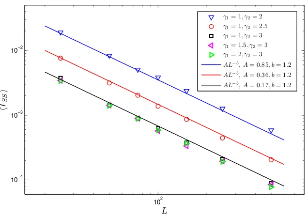
A novel finding of the explosive condensation process is that the time to stationarity

decreases with increasing system size. The scaled maximum occupancy numberηmax/N , which is the size of the site with the highest occupancy, is plotted against time in Fig. 3.3.

The system reaches stationarity when almost all particles are concentrated in one cluster.

The time to steady state is heuristically estimated to scale∼(lnL)1−γin [6]. This implies for L → ∞, steady state is reached instantly. The heuristic derivation of this intriguing result can be found in Appendix C, and a simpler novel alternative explanation will be introduced

in Chapter 4.

3.3 Tools to characterize explosive condensation

Studying the evolution of the maximum occupancy numberηmax, as outlined in the previous section, is one of the many methods in observing the various stages of explosive

conden-sation. The maximum occupancy number is the occupancy measurement of one single site

only, and it is not representative of the entire configuration. Step-by-step evolution of sys-tem configuration cannot be properly understood without a physical description of the entire

system configuration, such as the second momentσ2of the configuration. In Sec. 3.2, we

(40)

charac-0 0.5 1 1.5 x 10−3 0

0.2 0.4 0.6 0.8 1

t

ηm

ax

/N

L= 32

L= 64

L= 128

Figure 3.3: The scaled size of the largest cluster is plotted against time forγ = 5,d = 0.5 for the model with rates (3.1). Atηmas/N →0, all particles are concentrated on one cluster site.

terises explosive condensation, is also defined. The numerical efficiency and accuracy in

measuring a reliableTSSis also discussed in this section.

The stages to stationarity using such measurements are subsequently calculated

from the generator for theγ1 = γ2 = 1 case of the ECP or the inclusion process in Sec.

3.3.1. Attempts are made to repeat the same computation for the general ECP model, and discussions are provided to outline why this is ineffective. Note that the tools introduced in

this section will be used throughout this chapter and Chapter 4.

Maximum Occupancy

The simplest physical measurement is the maximum occupancyηmax, which is the

occu-pancy of the highest occupied site in the configurationη. This is defined as

ηmax=max

x∈Λ{η1, η2, ..., ηL}. (3.4) Although this is not a generic measurement for the entire system, the evolution of

the occupancy of the maximum siteηmax(t) can be a useful description for cluster-driven dynamics at the later stages of the dynamics (see Sec. 4.2). This is especially useful for cases with explosive condensation. This is because it provides an accurate measurement

of when the system reaches stationarity withηmax = (ρ −ρc)L, where only one cluster

(41)

Second momentσ2

The models of study are continuous time discrete space models, where for most cases a

non-equilibrium steady state contains the condensate. It is therefore advantageous to have global measurements, alongsideηmax, that characterise the system-wide distribution and are

not constrained for local measurement. The second momentσ2 across the system can be

measured and is defined as

σ2 ₌ 1 L

X

z∈Λ

η2

z . (3.5)

This is the simplest observable that captures the temporal evolution of the

con-densed phase, since the first moment is constant in time due to conservation of the number of particles. Due to spatial homogeneity, the expectation of (3.5) is equal to the expected

value ofη2x for all x. In simulations we approximate the expectation by averaging over

h1/LPL_x₌₁η2_xi, denoted byh·i(typically 100 in our simulations) of realizations. This is par-ticularly useful in studying the evolution of the system for coarsening dynamics (see Sec.

4.5.2), where several clusters dominate and a single condensate has not been formed yet.

However, we usehσ2iwith caution for monotonic increasing cases that are also extremely sensitive to waiting times. In fact, for some cases in Chapter 4, regular second moment

in-tervals are averaged over instead of averaging over regular time inin-tervals. This is discussed

in greater detail in Sec. 5.2.

Time to condensate

One of the main findings in ECP studies is that the time to steady state decreases withL [6, 59], such that forL → ∞, the time to steady stateT_SS → 0. The time to steady state is the time required for a system with particles that are initially distributed with uniform

probability on a site reaching its steady state.TSSis written as

T_SSσ2 =       

inft>0 n

t:σ2(t)>(ρ−ρc)2L−a

√

Lo , ifρ≥ρc

∞ , forρ < ρc ,

(3.6)

whereρc is the critical density of the system, such that when a condensate forms,ρcis the

background density anda√Lare the expected fluctuations of the system (see Sec. 4.5.1). Consistent with the characteristics of IPS with stationary product measures having

conden-sation in its steady state, (ρ− ρc)L is the expected mass of the condensate. The critical

densityρccan be predicted by the numerical computation of (2.14) (see Sec. 2.2.3).