1
Faculty of Electrical Engineering,
Mathematics & Computer Science
Direction-of-arrival estimation
of an unknown number of signals
using a machine learning framework
Noud B. Kanters M.Sc. Thesis January 2020
Supervisors:
Preface
This thesis has been written as the final part of my master’s programme Electrical Engineering at the university of Twente. The research presented in this document has been conducted within the Telecommunication Engineering chair and serves as their first investigation into the field of direction-of-arrival estimation aided by ma-chine learning.
I would like to thank my main supervisor Andr´es Alay´on Glazunov for the valuable discussions we had throughout the entire period of the assignment, as well as for his constructive feedback on this thesis. Furthermore, I would like to thank Chris Zeinstra for his input regarding the machine learning component of the work, an area completely new to me. Finally, I would like to express my gratitude to the members of the committee who assessed this thesis for their time.
Summary
Direction-of-arrival (DOA) estimation is a well-known problem in the field of array sig-nal processing with applications in, e.g., radar, sonar and mobile communications. Many conventional DOA estimation algorithms require prior knowledge about the source number, which is often not available in practical situations. Another common feature of many DOA estimators is that they aim to derive an inverse of the mapping between the sources’ positions in space and the array output. However, in general this mapping is incomplete due to unforeseen effects such as array imperfections. This degrades the performance of the DOA estimators.
In this work, a machine learning (ML) framework is proposed which estimates the DOAs of waves impinging an antenna array, without any prior knowledge about the number of sources. The inverse mapping mentioned above is made up by an ensemble of single-label classifiers, trained on labeled data by means of supervised learning. Each classifier in the ensemble analyses a number of segments of the discretized spatial domain. Their predictions are combined into a spatial spectrum, after which a peak detection algorithm is applied to estimate the DOAs.
The framework is evaluated in combination with feedforward neural networks, trained on synthetically generated data. The antenna array is a uniform linear array of 8 elements with half wavelength element spacing. A framework with a grid resolu-tion of 2◦, trained on105observations of 100 snapshots each, achieved an accuracy of 93% regarding the source number for signal-to-noise ratios (SNRs) of at least -5 dB when 2 uncorrelated signals impinge the array. The root-mean-square error (RMSE) of the estimates of the DOAs of these observations is below 1◦ and equals 0.5◦ for SNRs of 5 dB and higher. It is shown that in the remaining 7%, the DOAs are spaced 2.4◦ degree on average, making the resolution of the grid too coarse for resolving these DOAs.
Increasing the resolution of the grid is at the cost of an increased class imbal-ance, which complicates the classification procedure. Nevertheless, it is shown that a 100% probability of resolution is obtained for observations of 15 dB SNR with DOA spacings of at least 3.2◦ for a framework of 0.8◦ resolution, whereas the framework of 2◦ resolution achieves this for spacings larger than 5.9◦. However, 4 times more training data is used to realize this.
VI SUMMARY
A scenario with a variable source number showed that the performance of the ML framework decreases gradually with an increasing number of sources. When a single signal with a 15 dB SNR impinges the array, this is estimated correctly in 100.0% of the observations, with an RMSE of 0.4◦. However, when 7 sources exist, the performance decreases to 3.3% and 1.8◦ respectively. A decreased accuracy of the source number estimates was expected because of the 2◦ resolution that was used. However, it is shown that the performance of the neural networks in terms of their predictions decreases with an increasing source number as well.
Contents
Preface iii
Summary v
List of acronyms ix
1 Introduction 1
1.1 Goals of the assignment . . . 2
1.2 Related work . . . 2
1.3 Thesis organization . . . 3
2 Problem statement 5 2.1 Data model . . . 5
2.2 Assumptions and conditions . . . 7
3 Method 9 3.1 DOA estimation via classification . . . 9
3.2 The framework . . . 10
3.2.1 Label powerset . . . 11
3.2.2 RAkEL . . . 11
3.2.3 Modification 1 - combining RAkELoand RAkELd . . . 11
3.2.4 Modification 2 - border perturbations . . . 13
3.2.5 Modification 3 - peak detection . . . 14
3.3 The learning algorithm . . . 15
3.3.1 Topology . . . 15
3.3.2 Supervised learning . . . 17
3.3.3 Neural networks and the DOA-estimation framework . . . 17
4 Simulations and results 21 4.1 General simulation settings . . . 21
4.2 Constant, unknown number of sources . . . 23
VIII CONTENTS
4.2.2 Closely spaced sources . . . 27
4.2.3 Increasing the grid resolution . . . 30
4.2.4 Laplace distributed random DOAs . . . 33
4.3 Variable, unknown number of sources . . . 36
4.3.1 Uniformly distributed random DOAs . . . 37
5 Conclusions and recommendations 43 5.1 Conclusions . . . 43
5.2 Recommendations . . . 44
References 45 Appendices A Performance metrics 47 A.1 Classification performance . . . 47
A.2 RMSE . . . 49
A.3 Probability of resolution . . . 50
B Benchmarks 51 B.1 MDL and AIC . . . 51
B.2 Cram´er-Rao lower bound . . . 52
B.3 MUSIC . . . 53
C Additional results 55 C.1 Results for two sources . . . 55
C.1.1 Size of the training set . . . 55
C.1.2 Classifier performance . . . 57
C.1.3 Average DOA spacing . . . 61
C.1.4 Border perturbations . . . 61
C.2 Results for varying number of sources . . . 62
C.2.1 Confusion matrix . . . 62
D Mathematical derivations 63 D.1 RMSE for random DOA estimates . . . 63
D.2 Average spacing between neighbouring random DOAs . . . 64
D.3 RMSE for ideal classifiers without border perturbations . . . 64
List of acronyms
AIC Akaike information criterion AOA angle-of-arrival
BR binary relevance BWNN null-to-null beamwidth CRLB Cram´er-Rao lower bound DNN deep neural network DOA direction-of-arrival
ESPRIT estimation of signal parameters via rotational invariance techniques FFNN feedforward neural network
i.i.d. independent and identically distibuted LOS line-of-sight
LP label powerset
MDL minimum description length ML machine learning
MSE mean-square error
MUSIC multiple signal classification NN neural network
RAkEL randomk-labelsets
ReLU rectified linear unit rms root-mean-square
X LIST OF ACRONYMS
Chapter 1
Introduction
Estimating the direction-of-arrival (DOA), or angle-of-arrival (AOA), of multiple waves impinging a sensor array is a well-known problem in the field of array signal pro-cessing. It has a wide range of applications in, for example, radar, sonar and mobile communications. In practical situations, the number of sources is often unknown to the estimator, complicating the estimation process.
The DOA estimation problem has been addressed by, e.g., the popular subspace-based superresolution methods multiple signal classification (MUSIC) [1] and estimation of signal parameters via rotational invariance techniques (ESPRIT) [2]. However, both methods require prior knowledge about the source number. With an increasing amount of computational power being available, sparsity-based ap-proaches have become popular as well [3]. A common feature of the techniques mentioned above is that they rely on a model which maps the sources’ positions in space to the signals received by the sensor array. The DOA estimation is essentially a matter of finding the inverse of this mapping. However, in practice the forward mapping will contain imperfections because of, e.g., array imperfections, modelling errors in the sensors’ transfer functions, mutual coupling between the elements and the presence of noise. This will affect the inverse mapping as well, and with that degrade the performance of the DOA estimation algorithms.
As an alternative to computing an inverse mapping based on the (most likely) incomplete forward mapping, one could derive the inverse mapping directly from labeled input-output pairs, i.e. from real array outputs of which the corresponding source positions are known. As a result, factors such as array imperfections and the sensors’ transfer functions are included implicitly. This approach is called supervised learning, a well-known branch of machine learning (ML). This technique is the core of the assigment addressed in this thesis.
2 CHAPTER1. INTRODUCTION
1.1 Goals of the assignment
The main goal of the research presented in this thesis is summarized in the following statement:
Devise a machine learning framework which is able to estimate the directions-of-arrival of an unknown number of signals.
The idea behind this assignment is to find out the advantages, if any, of utilizing ML to solve this well-known DOA estimation problem. The work is not related to a particular application, meaning that no exact performance criteria are specified. Furthermore, no requirements regarding the ML algorithm or the antenna array are given. Ideally, the framework is constructed in a way that it can be employed in combination with any array configuration, such that it can be applied to both 1D and 2D DOA estimation.
1.2 Related work
Two well-known DOA estimation algorithms, both mentioned above, are MUSIC [1] and ESPRIT [2]. Whereas MUSIC is based on the noise subspace, ESPRIT employs the signal subspace. Both methods are by definition limited to estimating the DOAs of at most N −1 signals, with N being the number array elements. The number of
signals must be known before being able to estimate the DOAs. If the latter does not apply, it is to be estimated using, e.g., a subspace order estimator like the minimum description length (MDL) or Akaike information criterion (AIC) [4].
A. Khan et al. [5] combined the MUSIC algorithm [1] with several ML techniques for the 2D DOA estimation of a single target. It was shown that the DOA estima-tion performance in terms of mean absolute error improved aided by ML compared to using the MUSIC algorithm on its own. However, none of the considered ML techniques clearly outperformed the others.
In [6], 1D DOA estimation of two equally powered, uncorrelated sources using a deep neural network (DNN) was investigated. The DNN acts as a classifier with a 1◦ resolution and uses the estimated sensor covariance matrix of a 5-element uniform linear array (ULA) as an input. Only integer DOAs were considered. For a signal-to-noise ratio (SNR) of 30 dB, the estimation error was within 1◦ in 97% of the observations.
1.3. THESIS ORGANIZATION 3
whereas the support vector regression (SVR) method proposed in [8] resulted in errors upto 5◦ for the same scenario. The DNN was trained on a dataset consisting of 10 dB SNR observations only.
O. Bialer et al. [9] combined classification and regression in a single DNN. The neurons of the classifying part predict the number of sources, which is assumed to be between 1 and 4. Based on this prediction, a particular set of regression neurons containing the DOA estimates is to be read out. For a single snapshot, an SNR of 40 dB and an ULA of 16 elements, the probability that the number of sources is estimated correctly equals 90%.
1.3 Thesis organization
Chapter 2
Problem statement
In this chapter, the problem is formulated by means of a model based on well-known theoretical models presented in, e.g., [5], [7], [10], [11]. The data used for training and testing the ML framework is created using this model as well, as no real-world measurements were conducted within this assignment.
2.1 Data model
ConsiderK complex-valued narrow-band signals impinging an antenna array
con-sisting ofN isotropic elements. The sources transmitting these signals are assumed
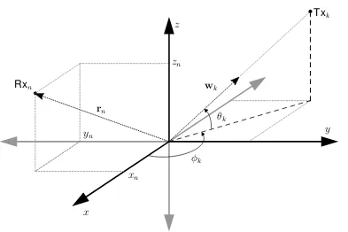
to be in the far-field of the array and the antenna elements of transmitters and re-ceiver are co-polarized. With yn(t) being the sample received by the nth element, i.e. n = 1, . . . , N, at thetth time instance, the data vectory(t) = [y1(t), . . . , yN(t)]T is modelled as
y(t) =As(t) +n(t), (2.1)
where y(t) ∈ CN, A ∈
CN×K is the array manifold, s(t) ∈ CK is a vector
contain-ing the complex amplitudes of the transmitted signals and n(t) ∈ CN is a vector containing the additive noise per antenna element.
The array manifold is given by
A= h
a1 a2 · · · aK
i
, (2.2)
where ak ∈ CN is the steering vector associated with the kth source, i.e. k =
1, . . . , K. Thekth steering vector is given by
ak =
h
a1,k a2,k · · · aN,k
iT
, (2.3)
and depends on the positions of the array elements relative to a reference point, the direction information of the signals, and the wavelengthλ. Thenth element of thekth
6 CHAPTER 2. PROBLEM STATEMENT
steering vector is defined as
an,k =e−j 2π
λr T
nwk. (2.4)
The vectorrn ∈R3 contains the Cartesian coordinates of thenth array element Rxn relative to the reference point
rn =
h
xn yn zn
iT
(2.5) and wk ∈ R3 is composed of the Cartesian coordinates of the unit-vector pointing from the reference point towards the kth source Txk. These Cartesian coordinates
are computed from the azimuth angleφk and the elevation angleθkas follows:
wk=
cosθk cosφk
cosθk sinφk
sinθk
. (2.6)
Without loss of generality, it is assumed that φ1 < · · · < φK and θ1 < · · · < θK. All geometry related parameters are visualized in Fig. 2.1.
x
z
φk
y
Txk
θk
wk
rn Rxn
xn
yn
[image:16.595.87.480.366.628.2]zn
Figure 2.1: Geometry definitions.
WhenT snapshots are available, i.e. t= 1, . . . , T, equation 2.1 can be written as
the matrix equation
Y=AS+N, (2.7)
2.2. ASSUMPTIONS AND CONDITIONS 7
2.2 Assumptions and conditions
Aided by the model described in section 2.1, the problem can be defined more specifically. The core of the problem is to estimate the DOAs of theK uncorrelated
narrow-band signals impinging the array, with K being unknown to the estimator.
The 2D DOA of the kth signal is defined by two parameters: the azimuth angle φk and the elevation angle θk. Each of the parameters mentioned above, i.e. K,
φk and θk (with k = 1, . . . , K), are assumed to be constant over all T snapshots within a single observation. Furthermore, it is assumed that boths(t) and n(t) are
independent and identically distibuted (i.i.d.) random variables following complex Gaussian distributions
s(t)∼ CN(0, σ2IK) (2.8a)
n(t)∼ CN(0, ν2IN)) (2.8b) withσ2 being the signal variance,ν2 the noise variance, andIK,I
N identity matrices of sizeK andN respectively. In other words, the DOA estimator has no knowledge
about the signals transmitted by the sources. Furthermore, equation 2.8 implies that all signals within a single observation have the same SNR, i.e. σ2/ν2.
Chapter 3
Method
Supervised learning algorithms can be roughly divided in two categories: classifica-tion algorithms and regression algorithms [12]. The core of the problem considered in this work is the unknown, possibly varying, number of sourcesK. This implies that
the number of target outputs of the framework could differ for various observations. Solving the problem using regression would therefore require a method similar to the one presented in [9], where the number of sources is predicted using a classifier prior to estimating the actual DOAs via regression. However, this implies that the design of the ML framework imposes a limit on the amount of DOAs that can be estimated. It was therefore decided to construct a framework which is solely based on classification and which does not need another algorithm to estimate the number of sources. This is achieved by discretizing the spatial domain, which comes at the cost of a finite estimation resolution. It was decided to consider 1D DOA estimation only, although the data model presented in section 2.1 could be used to generate 2D data as well. The azimuth angles φ1, . . . , φK are to be estimated, whereas the elevation anglesθ1, . . . , θK are fixed at 0 degrees. The principles behind the frame-work can be easily extended to 2D. The frameframe-work is presented in sections 3.1 and 3.2, whereas the employed learning algorithm is discussed in section 3.3.
3.1 DOA estimation via classification
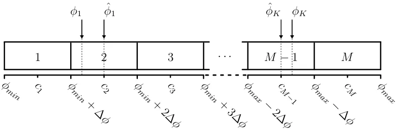
The first step towards estimating DOAs via classification is to define a grid. The spa-tial domain of interest,[φmin, φmax]withφmax > φmin, is divided inM equal segments. The width of one segment,∆φ, follows from
∆φ= φmax−φmin
M , (3.1)
for any positive integer M. If the DOA φ of a signal impinging the array is
asso-ciated with the ith segment, i = 1, . . . , M, its DOA estimate φˆ is the centre of that
10 CHAPTER 3. METHOD
segment,ci. The same procedure is used ifK signals impinge the array from angles φ1, . . . , φK, as visualised in Fig. 3.1. Note that if multiple DOAs correspond to the same grid segment, they cannot be resolved.
φ
min φmin
+ ∆ φ φ min + 2∆ φ φ min + 3∆ φ φ max − 2∆ φ φ max − ∆ φ φ max c
1 c2 c3 cM
− 1
c
M
· · ·
1 2 3 M −1 M
ˆ φ1
[image:20.595.86.480.155.284.2]φ1 φˆK φK
Figure 3.1: DOA estimation via classification.
The approach described above could be implemented using a label multi-class (or simply multi-label) multi-classifier: M classes exist of which K are true for a
single observation. In other words, K labels should be assigned. Multi-label
learn-ing problems have been investigated thoroughly. An overview of several methods to deal with this kind of ML problems is presented in [13]. A distinction is made be-tweenproblem transformationandalgorithm adaptationmethods. Algorithms in the former category transform the task into a more manageable problem such as binary classification or multi-class (single-label) classification. Techniques in the algorithm adaptation category are adapted versions of well-known ML algorithms, such that they can deal with multi-label data without transforming it.
As the problem statement of this thesis does not put any restriction on the ML al-gorithm to be used, a framework is proposed which can be combined with any single-label multi-class classification algorithm. In this way, different algorithms could be compared in a later stage. The framework is based on the ensemble method random
k-labelsets (RAkEL), proposed in [14]. RAkEL aims to achieve a high classification
performance while keeping computational complexity low. Section 3.2 presents how the RAkEL framework is employed to solve the given DOA estimation problem.
3.2 The framework
RAkEL is a framework which can be used to solve a multi-label classification
3.2. THE FRAMEWORK 11
3.2.1 Label powerset
LP is a technique which can be employed to transform a problem from multi-label to single-label [13]. It considers all 2M combinations of M possible labels. For example, for a multi-label classification problem with 2 labels, the LP consists of
22 = 4 classes. These classes are referred to as (00), (01), (10) and (11), where a 1 indicates that a label is assigned and a 0 denotes the opposite. Each digit represents one label. In this way, a single-label problem is obtained without losing information about possible correlations between the labels of the original multi-label task. The latter does not apply to, e.g., the binary relevance (BR) method, whereM
single-label classifiers are trained: one for each of theM labels. A disadvantage of
LP is that the number of classes grows exponentially withM. This complicates the
application of LP for domains with largeM as many classes will be represented by
few training examples [15]. The latter problem is addressed by RAkEL, as will be
shown in the next paragraph.
3.2.2 RA
k
EL
The main principle behind RAkEL [14] is the division of the single-label classification
problem of 2M classes in m smaller problems of 2k classes, i.e. k < M. This is achieved by splitting the original set of M labels in multiple subsets of k labels.
These subsets, from now on referred to as labelsets, are generated via random sampling from the original set. Single-label classifiers are trained on the LPs of those labelsets. Each label might or might not appear in multiple labelsets, referred to as RAkELo (overlapping) and RAkELd (disjoint) respectively. In other words, the
random sampling can be performed either with or without replacement. For RAkELo,
the final prediction for each label is obtained via a majority voting procedure over the entire ensemble. An example from [15] withm= 7,M = 6andk = 3is presented in
Table 3.1. The labelsc1, . . . , c6 can be considered as being the class centres shown in Fig. 3.1.
In [15], RAkEL is compared to 6 other multi-label learning techniques from both
the transformation as well as the adaptation category. It is shown that, averaged over 8 different databases, RAkELo withk = 3 andM < m < 2M outperforms the
considered techniques. Furthermore, it outperforms RAkELd for 7 of the 8
consid-ered databases.
3.2.3 Modification 1 - combining RA
k
EL
oand RA
k
EL
dA disadvantage of RAkELo is the imbalance in the amount of labelsets in which the
12 CHAPTER 3. METHOD
Table 3.1: RAkELo example [15]
Predictions
Classifier Labelset c1 c2 c3 c4 c5 c6
1 {c1,c2,c6} 1 0 - - - 1
2 {c2,c3,c4} - 1 1 0 -
-3 {c3,c5,c6} - - 0 - 0 1
4 {c2,c4,c5} - 0 - 0 0
-5 {c1,c4,c5} 1 - - 0 1
-6 {c1,c2,c3} 1 0 1 - -
[image:22.595.78.472.492.618.2]-7 {c1,c4,c6} 0 - - 1 - 0 Average votes 3/4 1/4 2/3 1/4 1/3 2/3 Final prediction 1 0 1 0 0 1
Table 3.1. This imbalance is a result of the random sampling and causes variations in the classification accuracy over the different labels: a label which appears in more labelsets will be assigned more accurately than labels covered by less classifiers in general. Furthermore, it could occur that certain labels are not selected at all. In the given DOA estimation application, this implies that specific sections of the spatial domain are not taken into account. This is unwanted, as a geometrically symmetric configuration of the sensors and sources should result in symmetric DOA estimation performance. It was therefore decided to useL’layers’ of RAkELdinstead
of RAkELo, as is visualized in Fig. 3.2. The labelsets consisting of k labels are
defined for each layer individually, as indicated by the shaded blocks.
k
layer 1 layer 2 layerL
...
φmin ∆φ φmax
· · · · · ·
k
2 1
· · ·
1
2 1
Figure 3.2:DOA estimation framework consisting of multiple layers of RAkELd.
The total number of classifiers m in the framework follows from the number of
layersL, the amount of labelsM and the number of labels in a labelsetk according
to
m=L &
M k
'
3.2. THE FRAMEWORK 13
3.2.4 Modification 2 - border perturbations
A disadvantage of the discretization of the spatial domain is that the estimation error
|φ−φˆ|approaches∆φ/2whenφapproaches the border between two segments. As
an additional result of the modification presented in section 3.2.3, this could be im-proved by making sure that the borders of different layers appear at different angles. It was therefore decided to perturb the borders for each RAkEL layer individually.
[image:23.595.109.497.250.377.2]An example of what the complete classifier framework could look like is shown in Fig. 3.3.
k
layer 1 layer 2 layerL
...
φmin ∆φ φmax
· · · · · ·
k
2 1
· · ·
1
2 1
Figure 3.3: DOA estimation framework with perturbed borders.
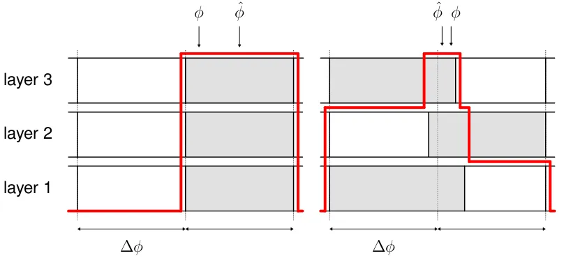
An artefact of these perturbations is that the DOA estimates can no longer be obtained via the straightforward majority voting procedure shown in Table 3.1. How-ever, the majority voting procedure can also be regarded as the comparison of some spectrum with the value L/2. This spectrum appears when summing the estimates
of all layers in the framework. This procedure can also be applied after perturbing the borders. The approach described above is illustrated by means of an example ofL= 3layers, shown in Fig. 3.4.
layer 1 layer 2 layer 3
∆φ ∆φ
[image:23.595.112.516.554.739.2]φ φˆ φˆ φ
14 CHAPTER 3. METHOD
The arrows labeled with ’φ’ represent a signal impinging the array from an
az-imuth angleφ. Each block in a layer represents a segment of the discretized spatial
domain. A shaded block indicates a positive estimate, i.e. the label of that grid seg-ment is assigned to the observation. Note that perfect classifiers are assumed in this example. By summing all estimates over the different layers, a spectrum (indi-cated by the red lines) appears. It can be seen that the perturbation of the borders (right) results in a DOA estimate φˆ(the middle of the peak plateau) which is closer
to the true DOA φ than the estimate that would be obtained without perturbations
(left). A more detailed explanation of how the DOA estimates follow from the spectra is presented in section 3.2.5.
3.2.5 Modification 3 - peak detection
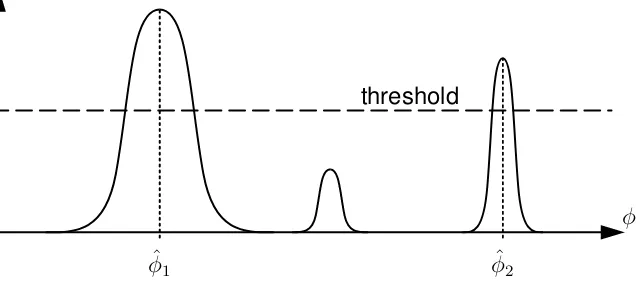
In section 3.2.4, it was shown how a spectrum is constructed based on the pre-dictions of the classifier ensemble. The DOA estimates are obtained by applying a peak detection algorithm to this spectrum. This algorithm computes all local maxima and compares them to some threshold. Only the peaks higher than the threshold are returned as being a DOA estimate. A threshold ofL/2can be interpreted as the
majority voting procedure usually applied in RAkELo, see Table 3.1. If a peak has
a flat top as in the example of Fig. 3.4, the argument of the centre of the plateau is taken as the estimate. The peak detection procedure is visualized in Fig. 3.5.
φ
threshold
ˆ
[image:24.595.113.433.466.607.2]φ1 φˆ2
Figure 3.5: Peak detection applied to a spatial spectrum.
Instead of using a fixed threshold, it was decided to optimize it using the data that is available. A set of calibration spectra is obtained by feeding the trained clas-sifier ensemble with observations it never saw before. These spectra, of which the associated parametersK andφ1, . . . , φK are known, can be evaluated using various threshold values. The value which maximizes the amount of observations for which
ˆ
K =K, withKˆ being the estimate ofK, is used as a threshold for new observations.
3.3. THE LEARNING ALGORITHM 15
A downside of this straightforward peak detection procedure is that two signals associated with two neighbouring segments of the grid cannot be resolved as they will result in a single peak. This might be taken into account by considering the width of the peak as well, which is a recommended investigation for the future. For now, two DOAs can only be resolved if their associated grid segments are separated by at least one other segment.
3.3 The learning algorithm
Given the framework presented in section 3.2, a base-level single-label learning al-gorithm is to be chosen. Examples of such alal-gorithms are decision trees, support vector machines and neural networks. Little literature is available in which the per-formance of different algorithms in the area of DOA estimation is compared. In [5] such a comparison is presented, but none of the three considered algorithms clearly outperforms the others. Furthermore, the scenario considered there is different, as the algorithms are trained on 2D MUSIC spectra. After all, it was decided to use the well-known feedforward neural network (FFNN) as a base-level algorithm. FFNNs come with a lot of design freedom and much literature has been published about using (deep) FFNNs for DOA estimation in the past few years, e.g. [7], [9], [10]. In spite of that, one of the recommendations for the future (section 5.2) would be to compare different algorithms within the framework presented earlier.
The remainder of this section consists of a description of the principles behind FFNNs. The topology of such a neural network (NN) is discussed first, followed by an explanation of the training and testing procedure. Finally, it is explained how they are employed within this assignment.
3.3.1 Topology
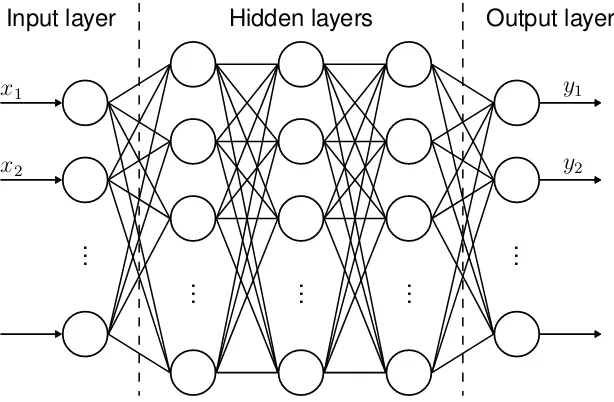
An FFNN consists of multiple layers: an input layer, one or more hidden layers and an output layer. Each of those layers contains one or more neurons. If each neuron in a layer is connected to all neurons in both the previous and the next layer, this layer is called fully-connected. Fig. 3.6 shows an example of an FFNN consisting of fully-connected layers. Note that the term ’feedforward’ in FFNN refers to the fact that no recurrent connections exist, such that information can travel in only one direction.
16 CHAPTER 3. METHOD
Hidden layers Output layer Input layer
y1
y2
x1
x2
...
[image:26.595.147.454.85.286.2]... ... ... ...
Figure 3.6:Fully connected feedforward neural network.
can be chosen freely. An approach to do this in a structured manner is presented in [12].
Each neuron of the network (except those in the input layer) comprises a se-quence of mathematical operations: all elements of the input vectorx0 = [x01, x02, . . .]T are multiplied with weighting factorsw01, w20, . . .. The next step is a summation of all
those products and, if desired, a bias term. The output of the summation is the input to a certain activation function. This function can be regarded as some kind of threshold, which produces a certain output y0 based on its input. Various
com-mon activation functions exist, but they might as well be user defined. A schematic overview of a neuron is shown in Fig. 3.7.
y0 x01
x02
...
P w01
w02
bias
f(·)
activation
Figure 3.7: Neuron.
[image:26.595.133.430.519.671.2]3.3. THE LEARNING ALGORITHM 17
3.3.2 Supervised learning
This paragraph contains a brief description of how an NN learns from data. As supervised learning is employed within this assignment, only this technique is con-sidered.
Supervised learning is the process of learning a mapping between input and output variables based on input-output pairs, i.e. input data of which the target output is known. The randomly initialized network predicts certain outputs based on the inputs of several input-output pairs. A loss function is used to assess the predictions by comparing them to the true targets. The more accurate the predictions, the lower the loss. An optimizer adjusts the parameters of the network based on the gradient of the loss such that the loss decreases in the next iteration. In order to reduce the computational load, one could use only subset (formally known as mini-batch) of the entire training set in each iteration. If the complete training set has been used once, one epoch has been completed.
In general, the training loss decreases every epoch. However, at some point the network does no longer improve the generic mapping from input to output, but it starts to overfit on the training data. This will degrade the performance of the NN for new observations. A validation set can be used to determine whether this is hap-pening. The data in the validation set is not used during the parameter optimization phase, but it is used to assess the performance of the network afterwards. Based on this assessment, the training process could be terminated. Furthermore, it could be decided to tune the hyperparameters of the network if the performance of the NN does not meet the requirements after training for many epochs. This means, however, that some information of the validation set leaks into the network as well, although implicitly. A third dataset, the test set, is therefore usually employed to get a fair assessment of the performance of the final network. The data in this set is completely new, i.e. none of the observations in this set appear in either the training or validation set. Before performing this final test, the network is usually trained from scratch using both the training and validation data.
3.3.3 Neural networks and the DOA-estimation framework
18 CHAPTER 3. METHOD
Input layer
The input to the NNs in the RAkEL framework is a vector of certain elements of the
estimated sensor covariance matrix Rb ∈ CN×N, similar to e.g. [6]. As the data is
created synthetically, this matrix is computed as
b
R= 1 T
T
X
t=1
y(t)yH(t)
= 1 T YY
H
(3.3)
withT, y(t)andY according to the data model presented in section 2.1. As Rb is a
Hermitian matrix, either the upper or lower triangle can be discarded without losing information. In other words, with ri,j being the element at row i and column j for
i, j = 1, . . . , N and·being the complex conjugate of an entry, it follows that
b
R=
r1,1 r1,2 · · · r1,N
r2,1 r2,2 · · · r2,N ... ... ... ...
rN,1 rN,2 · · · rN,N
, (3.4)
withri,j = rj,i. The shaded area in equation 3.4 indicates which elements are used as inputs to the NNs. As only real-valued scalars can be fed into a neuron, each off-diagonal element is associated with 2 neurons in the input layer: one for the real part and one for the imaginary part. In total, N diagonal elements and(N2 −N)/2
off-diagonal elements are used, resulting in N + 2(N2−N)/2 = N2 neurons in the
input layer. The input vectorx∈RN2
is constructed as follows:
x=r1,1 r2,2 · · · rN,N <(r1,2) <(r1,3) · · · =(r1,2) =(r1,3) · · ·
T
(3.5)
Hidden layers
All hidden layers in the networks are fully-connected. The activation function em-ployed in these layers is the rectified linear unit (ReLU) activation function. This is the most popular activation function in hidden layers of NNs nowadays [12]. The ReLU functionfReLU(u)is defined as
fReLU(u) = max(0, u) (3.6) withubeing the output of the summation shown in Fig. 3.7.
3.3. THE LEARNING ALGORITHM 19
Output layer
In section 3.2, it is explained that all classifiers in the ensemble have to deal with a 1-out-of-2k classification task. This explains why the NNs have 2k neurons in the output layer: one neuron for each class. The activation function used in the output layer is the softmax funtion. This function is used in many single-label multi-class classification problems. It is defined in such a way that the outputs of all neurons in the output layer add up to 1, such that they can be interpreted as a probability. The predicted class is the one with the highest probability. The output of theith neuron
in the output layer using the softmax activation functionfsm,i(u)withi = 1, . . . ,2k, is defined as
fsm,i(u) =
eui
P2k
j=1euj
. (3.7)
Here, u = [u1, . . . , u2k]T is a vector containing the outputs of all summations in the
output layer.
Training strategy
Instead of training all networks in the ensemble for a fixed amount of epochs, an early-stopping criterion is employed. If the loss of the validation set, monitored after every epoch, does not decrease anymore, the training stage is terminated. This prevents the networks from overfitting on the training data.
The parameters of the networks are optimized using the Adam optimizer [16] in combination with aweighted categorical cross-entropy loss function. Given a vector of target outputsv= [v1, . . . , v2k]T and a vectorvˆ = [ˆv1, . . . ,vˆ2k]T containing all
prob-abilities computed by the softmax activation function, the unweighted categorical cross-entropy lossDCE is defined as
DCE(v,vˆ) =
X
i
vilog(ˆvi) (3.8)
where i = 1, . . . ,2k. The definition of the softmax function is such that each
prob-ability in vˆ is nonzero, which means that the logarithm can always be computed.
The target vector contains only zeros except for a single 1 at the entry of the true class. The true class depends on the DOAs of the training observation as well as on the grid segments covered by the considered NN. For example, consider a spatial domain split inM = 4 segments: A,B,C and D. Assume one of the networks in the
ensemble coversk = 3 of those segments, e.g. A,B and D. Furthermore, assume K = 2 signals impinge the array, associated with classes A and C according to the
20 CHAPTER 3. METHOD
The DOA associated with segment C does not affect the target output, as this seg-ment is not covered by the considered network. If multiple DOAs would have been associated with segment A, the target vector would have been the same.
In the weighted version of the loss function, the loss of each of the2k classes is scaled by some factor. The reason for this is explained in the next paragraph.
Class imbalance
Before explaining the effect of assigning weights to the loss for each class individu-ally, the variableKN N is introduced. It is defined as the number of segments, out of the k segments considered a by certain NN, in which at least one signal impinges
the array. It holds that 0 ≤ KN N ≤ max(k, K). Considering k = 3 as an example, it follows that both KN N = 0 andKN N = 3 each represent 1 class: (000) and (111) respectively. On the other hand, KN N = 1 and KN N = 2 are both associated with 3 classes, being [(001), (010), (100)] and [(011), (101), (110)]. Since the labelsets are generated randomly, a single observation could correspond to different values ofKN N for different networks.
The spatial domain is divided in M segments (Fig. 3.1). In order to accurately
estimate the DOAs of K signals, it is required that K M. Assuming K signals
impinge the array from DOAs φ1, . . . , φK which are i.i.d. random variables of the uniform distributionU(φmin, φmax), it holds that
P(KN N = 0) =
M −k M
K
(3.9)
withkas defined in section 3.2.2 andP(KN N = 0)being the probability that a certain observation is associated with KN N = 0. It can be seen that a large M and a small
k and/orK result in a P(KN N = 0) close to 1. This implies that the majority of the observations will be associated with the single class corresponding toKN N = 0, i.e. (000). This phenomenon is called class imbalance.
The latter complicates the learning, as minorities are often neglected in classi-fication problems suffering from class imbalance [17]. One way to counteract this problem is to assign weights to the loss for erroneous predictions within the training stage. By making the weights inversely proportional to the support of the classes in the training set, all classes contribute equally much to the loss and the learning algorithm is forced to also focus on the minorities. More advanced techniques for dealing with class imbalance exist, see e.g. [17]. A future investigation could be to determine if the performance of the ML framework could be improved using such techniques.
Chapter 4
Simulations and results
Various simulations were conducted to assess the performance of the ML frame-work described in chapter 3. The frameframe-work is compared against a number of benchmarks by means of performance metrics such as the root-mean-square er-ror (RMSE) and the probability of resolution. Exact definitions of the performance metrics and the benchmarks are presented in appendices A and B respectively.
Section 4.1 contains a description of the simulation settings which apply to all simulations. Then, a scenario is considered in whichK is constant over all
obser-vations in section 4.2. This constraint is released in the simulations presented in section 4.3.
4.1 General simulation settings
Configuration
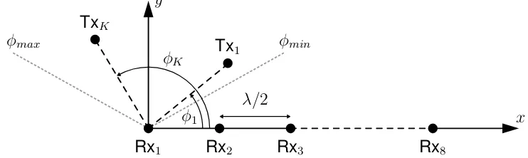
The antenna array used within all simulations is an ULA consisting ofN = 8isotropic
elements. The spacingdbetween the elements isλ/2. The array is positioned along
the x-axis, according to the definitions presented in Fig. 2.1. The DOAs of the K
signals impinging the array are referred to as φ1, . . . , φK, with φmin < φ1 < · · · <
φK < φmax. The configuration is visualised in Fig. 4.1.
Rx1 Rx2 Rx3 Rx8
λ/2
x y
TxK
φ1
φK
Tx1 φmin
[image:31.595.121.492.628.739.2]φmax
Figure 4.1: K signals impinge an8-element ULA.
22 CHAPTER4. SIMULATIONS AND RESULTS
Framework
The considered spatial domain [φmin, φmax] is [30◦,150◦]. It covers 120◦, which is common in hexagonal cellular networks. The RAkEL parameter k, i.e. the amount
of grid segments covered by each individual NN, is set to k = 3. This is suggested
in [15], as it is considered to be a good trade-off between performance and compu-tational complexity. The number of layers L (as described in section 3.2.3) equals
5, such that M < m < 2M, with M and m as defined in equations 3.1 and 3.2
respectively. The latter is another suggestion in [15], as they observed that increas-ing m to a value larger than 2M does not improve classification performance
any-more. The border perturbations are i.i.d. random variables of the uniform distribution
U(−∆φ/4,∆φ/4). The minimum width of a segment therefore equals∆φ/2.
Data
The data used for training and testing the ensemble of NNs is created using the data model presented in Chapter 2. The estimated sensor covariance matrices used as inputs to the NNs are computed from T = 100 snapshots. The DOAs φ1, . . . , φK of the training observations are i.i.d. random variables of the uniform distribution
U(φmin, φmax), unless stated otherwise. The SNR of the training observations is as-sumed to be a random variable following a discrete log-uniform distribution. In other words, the SNR expressed in dB has−20,−19, . . . ,30dB as possible values, all with
equal probability. The SNR of the test observations is either a log-uniform distributed random variable as well (with a step size of 5 dB), or a fixed value. This varies over the different simulations. If multiple signals impinge the array, they are assumed to have the same power and therefore the same SNR, as already mentioned in sec-tion 2.2.
Machine learning
The input layer of all NNs consists ofN2 = 64neurons, whereas2k= 8 neurons are
4.2. CONSTANT,UNKNOWN NUMBER OF SOURCES 23
4.2 Constant, unknown number of sources
In this section, it is assumed thatK = 2for all observations in both the training and
the test set. The latter is unknown to the estimator.
The results presented in sections 4.2.1 and 4.2.2 are obtained using a framework with a grid resolution of∆φ = 2◦. The DOAs for the observations in the test set used
in section 4.2.1 are uniformly distributed random variables as well. In section 4.2.2, a different test set is used in order to investigate closely spaced sources in more detail. In section 4.2.3,∆φis decreased to 0.8◦ to investigate the impact of increasing the
resolution of the framework. Finally, section 4.2.4 contains a discussion of how the framework could be adapted to the data if the DOAs are not uniformly distributed.
4.2.1 Uniformly distributed random DOAs
The results presented in this section are obtained using a grid resolution of ∆φ = 2◦. Given that φmax −φmin = 120◦, L = 5 and k = 3, this yields an ensemble of
m = 100 NNs (equations 3.1 and 3.2). All NNs in the ensemble have 2 hidden
layers, one of 64 and one of 36 neurons. Based on empirical research presented in appendix C.1.1, it was observed that training on105observations is sufficient for this specific scenario. The test set consists of1.5×104 observations for each evaluated SNR.
A detailed analysis of the classification performance of the NNs is presented in appendix C.1.2. The analysis confirms that the classifiers suffer from a significant class imbalance, as about 90.3% of the observations are associated withKN N = 0. This was expected based on equation 3.9. Furthermore, it is observed that the majority of incorrect predictions for observations associated with KN N > 0 implies that a label is not assigned where it should have been, rather than vice versa. This is advantageous, as this merely implies that spectrum peaks are lower than they would have been with perfect classifiers. As the threshold of the peak detection algorithm is adapted to the spectra, the ML framework could, theoretically, compensate for this. Whether it does, is evaluated using a metric relevant in the field of DOA estimation, being the RMSE (appendix A.2). The RMSE is evaluated for both the ML framework and the MUSIC algorithm (appendix B.3). The resolution of the MUSIC algorithm is 0.1◦.
The definition of the RMSE is such that it can only be computed if Kˆ = K, i.e.
if the estimated number of signals equals the true number of signals. This makes the probability that this is the case, P( ˆK = K), a relevant parameter to consider.
For the ML framework, Kˆ is defined as the amount of spectrum peaks higher than
spa-24 CHAPTER4. SIMULATIONS AND RESULTS
tial spectrum. However, the MUSIC algorithm (and many other DOA estimation algorithms) requires an estimate ofK beforeactually being able to start the compu-tations. The probability P( ˆK =K)is therefore evaluated for both the ML framework
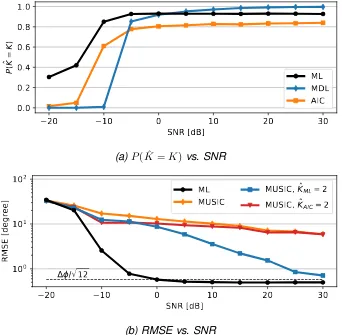
and two subspace order estimators: the MDL and AIC [4] (appendix B.1). For ease of notation, they will be referred to as, P( ˆKM DL = K) and P( ˆKAIC = K) respec-tively, whereasP( ˆKM L =K)denotesP( ˆK =K)for the ML framework. The RMSE and theP( ˆK =K), plotted against the SNR, are shown in Fig. 4.2.
20
10
0
10
20
30
SNR [dB]
0.0
0.2
0.4
0.6
0.8
1.0
P(
K=
K)
ML
MDL
AIC
(a)P( ˆK=K)vs. SNR
20
10
0
10
20
30
SNR [dB]
10
010
110
2RMSE [degree]
/ 12
ML
MUSIC
MUSIC, K
MUSIC, K
MLAIC= 2
= 2
[image:34.595.114.456.229.564.2](b) RMSE vs. SNR
Figure 4.2: DOA estimation metrics,K = 2,1.5×104 observations per SNR.
As can be observed in Fig. 4.2a,P( ˆKM L =K)increases with the SNR of the ob-servations, until it stabilizes at 93% for SNRs of -5 dB and higher. In appendix C.1.3, it is shown that the average spacing between the DOAs in observations for which
ˆ
4.2. CONSTANT,UNKNOWN NUMBER OF SOURCES 25
SNRs, the ML framework correctly estimates the number of signals in 81.8% of the cases, contrary to 69.8% for the MDL. The difference of 12% mainly originates from SNRs smaller than -5 dB. Looking at the RMSE of the framework for these SNRs, (Fig. 4.2b), it can be seen that it approaches 40◦. This is the RMSE that would be obtained when estimating the DOAs using sorted uniformly distributed random vari-ables (appendix D.1): (φmax −φmin)/
p
3(K+ 1) = 120◦/p3(2 + 1) = 40◦. In other
words, the DOA estimates at these SNRs hardly contain information.
For SNRs of -5 dB and higher, the RMSE of the DOA estimates of the ML frame-work is below 1◦. For SNRs of 0 dB and higher, it is below ∆φ/√12≈ 0.58◦, which is the RMSE that would be obtained when employing the framework in combination with ideal classifiers without the border perturbations introduced in section 3.2.4 (ap-pendix D.3). This suggests that the border perturbations benefit the DOA estimates, which is confirmed by running another simulation of the same scenario with border perturbations turned off (appendix C.1.4). The difference between the two frame-works in terms of the RMSE is between 0.1◦ and 0.2◦ for SNRs of 5 dB and higher, in favour of the frameworkwithperturbed borders.
Returning to the RMSE presented in Fig. 4.2b, it can be observed that three graphs are plotted for the MUSIC algorithm. These graphs are obtained by comput-ing the RMSE for
1. all observations, i.e. assuming some perfectK-estimator exists;
2. all observations for whichKˆ
M L =K = 2; 3. all observations for whichKˆAIC =K = 2.
It was decided to use the AIC instead of the MDL asP( ˆKAIC =K)>0for all SNRs. When considering graph 3 from the list above, i.e. the red graph in Fig. 4.2b, it can be seen that the difference between the ML framework and MUSIC, in terms of the RMSE, is at least a factor 10 for all SNRs of -5 dB and higher (in favour of the ML framework). Combining this with Fig. 4.2a, it can be concluded that the ML framework outperforms the combination MUSIC + AIC: neglecting the -20 dB SNR for which the RMSEs of both algorithms approach the RMSE obtained by random guessing, it both holds thatP( ˆKM L =K)> P( ˆKAIC =K)as well as that the RMSE is lower for the ML framework than for MUSIC.
It is important to realise that the observations for which KˆM L = 2 and those for
which KˆAIC = 2 are not the same, as can be concluded from Fig. 4.2a. A more
fair comparison between MUSIC and the ML framework is therefore obtained by applying MUSIC to those observations for which KˆM L = 2 (graph 2 from the list
26 CHAPTER4. SIMULATIONS AND RESULTS
the RMSE of the ML framework with an increasing SNR. For an SNR of 30 dB the difference is only 0.2° , still in favour of the ML framework.
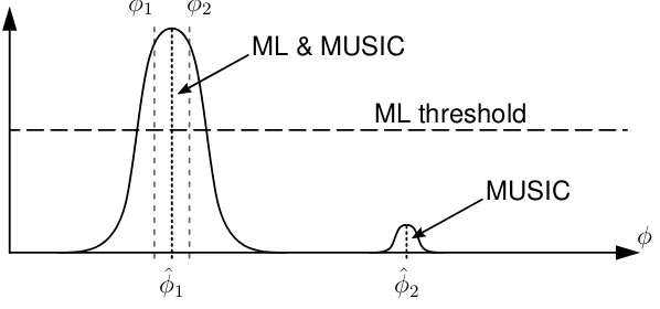
[image:36.595.123.422.181.321.2]After a closer inspection of these results, it was observed that observations with closely spaced sources dominate the RMSEs for the MUSIC algorithm presented in Fig. 4.2b. The latter is explained using a fictitious example, visualised in Fig. 4.3.
φ
ML threshold
ˆ
φ1 φˆ2
φ1 φ2
MUSIC ML & MUSIC
Figure 4.3: Closely spaced DOAs result in a larger RMSE for MUSIC compared to the ML framework.
The DOAs in this example, φ1 and φ2, are closely spaced. Due to the noisy estimate of the sensor covariance matrix employed by both MUSIC and the ML framework and the finite resolution that comes with both methods, the desired peaks in the spatial spectrum merge into a single peak such that the DOAs cannot be resolved. It is assumed that this applies to the spectra computed by both the ML framework and the MUSIC algorithm.
In this situation, the ML framework will return only a single DOA estimate (φˆ1) as
there is only one peak in the spectrum which is higher than the threshold. However, the MUSIC algorithm is told by some other algorithm that K = 2 signals impinge
the array. It will therefore select the 2 highest peaks of the spectrum and return their arguments as the DOA estimates (φˆ1,φˆ2), even if the second peak is much lower and
located at an irrelevant angle. The latter results in large estimation errors dominating the RMSE.
If, for an experiment with closely spaced DOAs, the ML framework successfully resolves the 2 signals whereas MUSIC does not, this will affect the RMSE for MUSIC because of the above. However, when the opposite applies, the experiment is dis-carded asKˆM L 6=K such that no RMSE can be computed. The latter applies to the
7% of the observations with SNRs of -5 dB and higher for which the average DOA spacing is 2.8◦ or less.
4.2. CONSTANT,UNKNOWN NUMBER OF SOURCES 27
4.2.2 Closely spaced sources
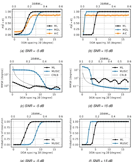
In this paragraph a symmetric scenario is considered in which φ1 = 90−δ degree and φ2 = 90 +δ degree. The spacing between the two signals, φ2 −φ1 = 2δ is increased gradually. Note that this only applies to the test data. The training data is as described in section 4.2.1. Besides the metrics RMSE andP( ˆK =K), the
prob-ability of resolution is evaluated as well (appendix A.3). The latter metric combines the estimation error and P( ˆK = K) into a single number. Two different SNRs are
considered, being -5 dB and 15 dB.
The results are presented in Fig. 4.4. Each data point is the average of 5000 observations. Note that the upper x-axes show the DOA spacing relative to the null-to-null beamwidth (BWNN) of the antenna array. Conventional methods such as the beamscan method cannot resolve DOAs with spacings smaller than BWnn/2 [18]. For the array employed in this work,BWnn ≈28.96◦(appendix A.3). The vertical grid, shown in all images, represents the spatial grid which is inherent to the framework (neglecting the perturbed borders). In other words, each vertical line indicates that the spacing between the DOAs has increased by 2∆φ = 4◦. The grid resolution is
important, as two closely spaced sources can only be resolved if they are separated by at least one grid segment, as explained in section 3.2.4.
In Fig. 4.4a (-5 dB) and Fig. 4.4b (15 dB), P( ˆK = K) is shown for both the ML
framework as well as for the benchmarks MDL and AIC. Comparing both images, it can be observed that both the MDL and the AIC reach their maximumP( ˆK =K)at
smaller separations for the higher SNR. To a lesser extent, this also applies to the ML framework: P( ˆK = K) = 1 for spacings larger than 7.4◦ (-5 dB) and 5.9◦ (15
dB). For the 15 dB case,P( ˆKM L = K) rises from 0 to 1 as soon as the DOAs are separated by at least 1 grid segment (in this case 2 segments, due to symmetry). The fact that the rise of the edge initiates at slightly smaller separations could be explained by the border perturbations and/or erroneous predictions of the NNs. The slope of the graph of the -5 dB case is more gradual. For this SNR, P( ˆKM L =
K) > 0 for all evaluated separations, even those smaller than 2∆φ. This does not
imply that the ML framework performs better for the -5 dB case though, as it was already reasoned in section 3.2.4 that resolving DOAs with such small separations is theoretically impossible if the classifiers are perfect. The RMSE confirms that false predictions of the classifiers are the cause of the fact thatP( ˆKM L =K)>0for separations smaller than2∆φ.
28 CHAPTER4. SIMULATIONS AND RESULTS
0
5
10
15
DOA spacing 2 [degree]
0.00
0.25
0.50
0.75
1.00
P(
K=
K)
ML
MDL
AIC
0.0
0.2
2 /BW
nn0.4
0.6
(a) SNR = -5 dB
0
5
10
15
DOA spacing 2 [degree]
0.00
0.25
0.50
0.75
1.00
P(
K=
K)
ML
MDL
AIC
0.0
0.2
2 /BW
nn0.4
0.6
(b) SNR = 15 dB
0
5
10
15
DOA spacing 2 [degree]
10
010
1RMSE [degree]
ML
MUSIC
CRLB
0.0
0.2
2 /BW
nn0.4
0.6
(c) SNR = -5 dB
0
5
10
15
DOA spacing 2 [degree]
10
110
010
1RMSE [degree]
ML
MUSIC
CRLB
0.1
0.2
0.3
2 /BW
0.4
nn0.5
0.6
(d) SNR = 15 dB
0
5
10
15
DOA spacing 2 [degree]
0.00
0.25
0.50
0.75
1.00
Probability of resolution
ML
MUSIC
0.0
0.2
2 /BW
nn0.4
0.6
(e) SNR = -5 dB
0
5
10
15
DOA spacing 2 [degree]
0.00
0.25
0.50
0.75
1.00
Probability of resolution
ML
MUSIC
0.0
0.2
2 /BW
nn0.4
0.6
[image:38.595.68.500.138.668.2](f) SNR = 15 dB
4.2. CONSTANT,UNKNOWN NUMBER OF SOURCES 29
of the ML framework for the -5 dB case, it can be observed that it is bigger than 1◦ for separations smaller than 2∆φ (i.e. left of the second vertical grid line). As the resolution of the framework ∆φ = 2◦, the maximum RMSE would be 1◦ for
ideal classifiers. It can therefore be concluded that P( ˆK = K) > 0 for these small
separations results from erroneous predictions of the NNs. Despite these errors, the ML framework clearly outperforms MUSIC for separations smaller than 0.4BWnn.
For larger separations, the framework seems to be limited by its grid resolution of 2◦. The fact that the RMSE of the ML framework is lower than the CRLB indicates that the framework is biased. This is inherent to the discrete grid on which the framework is based, as DOA estimates will either be the centre of a grid segment, or some angle close to the border between two classes.
For the 15 dB case, MUSIC outperforms the ML framework (in terms of the RMSE) for nearly all separations. The impact of the finite resolution of the frame-work can be observed, as the peaks and valleys in its graph align with the segment borders and segment centres respectively. However, the RMSE is below 1◦ for all peaks, confirming once more that the border perturbations benefit the DOA esti-mates. A maximum improvement of 0.4◦ is observed (0.6◦ instead of 1◦ at the 4th vertical grid line). Finally it can be seen that the RMSE for MUSIC cannot follow the CRLB for separations larger than approximately0.3BWnn. This can be explained by
the 0.1◦ resolution of the scanangles at which the MUSIC spectra are evaluated. The probability of resolution is depicted in Fig. 4.4e and Fig. 4.4f. For the -5 dB scenario, the ML framework achieves 100% at DOA spacings of at least 7.4◦, con-trary to 11.6◦ for the MUSIC algorithm. For separations smaller than 0.1BWnn, the DOAs are never resolved. However, P( ˆKM L =K) >0for these spacings, implying that the estimates are not accurate enough. The reader is referred to the definition of the probability of resolution (appendix A.3) for a formal definition of ’accurate’. For the 15 dB case, the ML framework resolves both signals in all observations if the spacing is at least 5.9◦, contrary to 3.5◦ for MUSIC. Note that the probability of resolution is identical to P( ˆKM L = K) (Fig. 4.4b) for this SNR. In other words, if the source number is estimated correctly, the DOA estimates are accurate as well. Note that the results shown for MUSIC assume that a perfect K-estimator exists.
In practice, MUSIC can only be applied in combination with, e.g. a subspace order estimator, meaning that the probability of resolution could be lower than shown here. It can be concluded that the ML framework outperforms the MUSIC algorithm regarding closely spaced sources for an SNR of -5 dB, whereas the opposite holds for 15 dB. For the latter SNR, the resolution of the framework seems to be a limiting factor, as bothP( ˆKM L=K)and the probability of resolution rise from 0 to 1 as soon as the spacing exceeds2∆φ. Whether increasing the resolution could improve the
30 CHAPTER4. SIMULATIONS AND RESULTS
4.2.3 Increasing the grid resolution
Based on the results presented in sections 4.2.1 and 4.2.2, it was decided to investi-gate if increasing the resolution of the framework, i.e. decreasing∆φ, could increase
its performance. Decreasing ∆φ implies an increased amount of grid segmentsM
(equation 3.1). Considering uniformly distributed random DOAs with K = 2 (as in
section 4.2.1), it follows that P(KN N = 0)increases as well (equation 3.9). In other words, increasing the resolution of the framework comes with an increase of the class imbalance. Less observations will therefore be associated with the minority classes, i.e. classes of the clusters KN N = 1and KN N = 2, if the size of the train-ing set is kept the same. Learntrain-ing an accurate mapptrain-ing for these classes therefore becomes more and more complex with smaller values of ∆φ.
Despite an increase of M, the task of each classifier (in this work NN) in the
ensemble remains the same: picking the correct class out of 2k possible classes. In other words, if the networks in a framework with increased resolution achieve similiar behaviour as the networks in the 2◦ resolution framework, the RMSE would
automatically decrease. Furthermore, it would imply that closely spaced DOAs could be resolved for smaller spacings, i.e. that the graph representing the ML framework in Fig. 4.4f shifts to the left. Assuming the latter holds, it can be observed that a grid resolution of ∆φ = 0.8◦ would be sufficient to outperform the MUSIC algorithm in
terms of the probability of resolution at an SNR of 15 dB.
In Fig. 4.5, two frameworks are compared: the framework with a resolution of
∆φ = 2◦ employed in sections 4.2.1 and 4.2.2, and a ’high resolution’ framework
with∆φ = 0.8◦. Based on empirical research, it was decided to increase the training
set for the latter framework to4×105observations. Furthermore, the network layout
is increased to 3 hidden layers, consisting of 84, 84 and 36 neurons.
Besides the conventional DOA estimation metrics RMSE and P( ˆK = K), the
performance of both frameworks is evaluated by means of the metrics precision and recall as well (appendix A.1). These are measures for the classifiers’ exactness and completeness respectively. In other words, they are an indication of the quality of the predictions performed by the NNs, before they are converted to DOA estimates. By definition, both metrics are computed for each of the2kclasses individually. Classes
4.2. CONSTANT,UNKNOWN NUMBER OF SOURCES 31
20 10 0 10 20 30
SNR [dB] 0 20 40 60 80 100
Precision KKNNNN= 0, = 2= 0, = 0.8
KNN= 1, = 2
KNN= 1, = 0.8
(a) Precision
20 10 0 10 20 30
SNR [dB] 0 20 40 60 80 100
Recall KNN= 0, = 2
KNN= 0, = 0.8
KNN= 1, = 2
KNN= 1, = 0.8
(b) Recall
20 10 0 10 20 30
SNR [dB] 100 101 RMSE [degree] = 2 = 0.8
0 10 20 30
0.25 0.50
(c) RMSE
20 10 0 10 20 30
SNR [dB] 0.0 0.2 0.4 0.6 0.8 1.0 P( K= K) = 2 = 0.8
0 10 20 30
0.925 0.950 0.975
[image:41.595.92.528.88.399.2](d)P( ˆK =K)
Figure 4.5: Performance metrics for frameworks of∆φ= 2◦ and∆φ= 0.8◦.
the higher resolution (appendix D.4). The precision and recall are shown in Fig. 4.5a and Fig. 4.5b respectively.
It can be observed that both the precision and the recall for observations corre-sponding toKN N = 0are at least 97% for SNRs of -5 dB and higher, for both res-olutions. A high performance was to be expected, as classifiers are biased towards the majority class in problems with a significant class imbalance [17]. It implies that the framework is good at estimating at which angles signalsdo not impingethe ar-ray. However, the classes of the clusterKN N = 1 are most important to decide from which angles signals do impinge the array, as correct predictions for observations corresponding to these classes will result in peaks in the spectra at the correct an-gles. For classes of this cluster, the precision of the 0.8◦ resolution framework is
above 78.4% for SNRs of 10 dB or higher, with a maximum of 80.7% for an SNR of 30 dB. The NNs in the low resolution framework achieved a precision above 86.2% for SNRs of at least 10 dB. A similar trend is observed for the recall, although the differences are bigger. For SNRs of at least 5 dB, the recall was above 82.5% for the low resolution framework, whereas it is between 63.2% and 68.7% after increasing the resolution.
32 CHAPTER4. SIMULATIONS AND RESULTS
can be observed that increasing the resolution has reduced the RMSE, with a dif-ference of about 0.25◦ for SNRs of 10 dB and higher. However, the minimum RMSE achieved (0.25◦) is not below the RMSE for perfect classifiers without perturbations,
∆φ/√12 = 0.8◦/√12 ≈ 0.23◦. The low resolution framework did achieve this limit
(0.50◦ vs. 0.58◦, appendix D.3). The probability that Kˆ = 2(Fig. 4.5d) improved as well, as it increased by about 3% for SNRs of 0 dB and larger. The fact that it de-creased for the lowest SNRs does not matter, as the RMSE indicates that the DOA estimates at these SNRs do not contain information anyway. Note that for SNRs of 0 dB and higher, Kˆ = 2 for more than 95% of the observations with and RMSE
below 0.5◦, while for the same SNRs, the precision is between 65.1% and 80.7% and the recall between 53.9% and 68.7%. Since each grid segment is covered by
L= 5classifiers and the threshold of the peak detection algorithm is adapted to the
data, the framework successfully compensates for the relatively low performance of the classifiers.
The origin of the increase in P( ˆK = K) can be explained by investigating the
probability of resolution for closely spaced sources once more. It is evaluated for the frameworks of both resolutions, as well as for the MUSIC algorithm. The results are shown in Fig. 4.6.
1
2
3
4
5
6
7
8
9
DOA spacing 2 [degree]
0.00
0.25
0.50
0.75
1.00
Probability of resolution
ML, = 0.8
ML, = 2
MUSIC
= 0.8
= 2.0
[image:42.595.95.475.425.574.2]0.05
0.10
2 /BW
0.15
nn0.20
0.25
0.30
Figure 4.6: Probability of resolution for various∆φ, SNR = 15 dB.
The two vertical grid lines represent a DOA spacing of2∆φ. It can be observed
that, similar to the low resolution framework, the probability of resolution for the high resolution framework rises from 0 to 1 as soon as the DOA separation has increased beyond2∆φ. The high resolution framework achieves a 100% probability
4.2. CONSTANT,UNKNOWN NUMBER OF SOURCES 33
difference between MUSIC and the high resolution ML framework is obtained at a DOA spacing of 2◦, where the ML framework achieves a probability of resolution of 63%, contrary to 11% for MUSIC.
It can be concluded that the performance of the ML framework can be increased by increasing its resolution, although this is at the expense of more training data being required, at least for the data, learning algorithm, training strategy, etc. con-sidered here. A recommendation for the future would be to investigate if the need for extra training data could be diminished by advanced class imbalance techniques such as oversampling or synthetic data generation [17]. Furthermore, it would be useful to find a relation between the performance of the classifiers, e.g. in terms of the classification metrics presented in appendix A.1, and the DOA estimation perfor-mance metrics RMSE andP( ˆK =K). The results presented in this section (Fig. 4.5
specifically) indicate correlation between the two, but further research is required to determine the impact of, e.g., the number of layers L in the framework. If such
a relation is known, one could use the validation set to determine (already during training stage) if satisfactory DOA estimation performance will be achieved for the considered settings (grid resolution, training strategy, etc).
4.2.4 Laplace distributed random DOAs
In this final paragraph of the current section, the DOAs of the signals are no longer assumed to be uniformly distributed over the spatial domain. Instead, it is assumed that they are Laplacian distributed, as this is the most common model for the angular dispersion at a base station [19]. In [20], it is stated that the root-mean-square (rms) angular spreadσ for line-of-sight (LOS) situations in a microcell is typically between
5◦ and 20◦. With the distribution being centred around the mean µ, the pdf f(x) of the Laplace distribution is defined as
f(x) = √1
2σ exp
− √
2|x−µ|
σ
(4.1)
with supportx∈R. Its cdfF(x)is defined as
F(x) = 1 2exp
√2(x−µ)
σ
ifx≤µ
1−1 2exp
− √
2(x−µ) σ
ifx > µ
(4.2)
![Table 3.1: RAkELo example [15]Predictions](https://thumb-us.123doks.com/thumbv2/123dok_us/9591525.462715/22.595.120.450.94.265/table-rakelo-example-predictions.webp)