http://wrap.warwick.ac.uk/
Original citation:
Diakonos, F. K., Karlis, A. K. and Schmelcher, P.. (2014) A universal mechanism for
long-range cross-correlations. EPL (Europhysics Letters), Volume 105 (Number 2).
26004. ISSN 0295-5075
Permanent WRAP url:
http://wrap.warwick.ac.uk/59701
Copyright and reuse:
The Warwick Research Archive Portal (WRAP) makes this work by researchers of the
University of Warwick available open access under the following conditions.
This article is made available under the Creative Commons Attribution 3.0 Unported (CC
BY 3.0) license and may be reused according to the conditions of the license. For more
details see:
http://creativecommons.org/licenses/by/3.0/
A note on versions:
The version presented in WRAP is the published version, or, version of record, and may
be cited as it appears here.
This content has been downloaded from IOPscience. Please scroll down to see the full text.
Download details:
IP Address: 137.205.202.117
This content was downloaded on 07/03/2014 at 08:40
Please note that terms and conditions apply.
A universal mechanism for long-range cross-correlations
View the table of contents for this issue, or go to the journal homepage for more 2014 EPL 105 26004
(http://iopscience.iop.org/0295-5075/105/2/26004)
January 2014
EPL,105(2014) 26004 www.epljournal.org
doi: 10.1209/0295-5075/105/26004
A universal mechanism for long-range cross-correlations
F. K. Diakonos2, A. K. Karlis1,2 andP. Schmelcher3,4
1 Department of Physics, University of Warwick - Coventry CV4 7AL, UK 2 Department of Physics, University of Athens - GR-15771 Athens, Greece
3 Zentrum f¨ur Optische Quantentechnologien, Universit¨at Hamburg - Luruper Chaussee 149,
D-22761 Hamburg, Germany
4 The Hamburg Centre for Ultrafast Imaging - Luruper Chaussee 149, D-22761 Hamburg, Germany
received 16 September 2013; accepted in final form 16 January 2014 published online 11 February 2014
PACS 64.70.qj– Dynamics and criticality
PACS 05.45.Ac– Low-dimensional chaos
PACS 05.45.Pq– Numerical simulations of chaotic systems
Abstract– Cross-correlations are thought to emerge through interaction between particles. Here we present a universal dynamical mechanism capable of generating power-law cross-correlations between non-interacting particles exposed to an external potential. This phenomenon can occur as an ensemble property when the external potential induces intermittent dynamics of Pomeau-Manneville type, providing laminar and stochastic phases of motion in a system with a large number of particles. In this case, the ensemble of particle-trajectories forms a random fractal in time. The underlying statistical self-similarity is the origin of the observed power-law cross-correlations. Furthermore, we have strong indications that a sufficient condition for the emergence of these long-range cross-correlations is the divergence of the mean residence time in the laminar phase of the single particle motion (sporadic dynamics). We argue that the proposed mechanism may be relevant for the occurrence of collective behaviour in critical systems.
open access Copyright cEPLA, 2014
Published by the EPLA under the terms of the Creative Commons Attribution 3.0 License (CC BY). Further distribution of this work must maintain attribution to the author(s) and the published article’s title, journal citation, and DOI.
Complex systems usually consist of several dynamical components interacting in a non-linear fashion. Cross-correlations are then used in order to explore the inter-dependence in the time evolution of these components measured in terms of specific quantities characterizing each component. In this context, the existence of cross-correlations has been demonstrated in a wide class of dynamical systems ranging from nano-devices [1] to atmo-spheric geophysics [2], seismology [3], finance [4–8], phys-iology and genomics [8]. Of special interest is the case of long-range (power-law) cross-correlations (LRCC) which, being scale free, may be associated with the appearance of characteristics of criticality in the dynamics of the consid-ered complex system. Such a behaviour has been observed, among other examples, in price fluctuations of the New York Stock Exchange during crisis [8], physiological time-series of the Physiology Sleep Heart Health Study (SHHS) database [8], the spatial sequence describing binding prob-ability of DNA-binding proteins to genes at different loca-tions on mouse chromosome 2 [8] and in flocks of birds [9]. All these findings indicate that the presence of
power-law cross-correlations is a quite general property of the dynamics of complex systems. Even more, very recently geometry-induced power-law cross-correlations have been also observed in a coarse-grained description of the dy-namics of an ensemble of non-interacting particles prop-agating in a Lorentz channel [10]. This clearly poses the question of the origin and mechanisms of cross-correlations in particle systems.
Up to now the theoretical treatment of cross-correlations is based on statistical approaches and their microscopic origin is to a large extent unclear. In the following, we identify the dynamical mechanisms leading to LRCC and show specifically that intermittent dynam-ics, characterized by long intervals of regular evolution (laminar phases) interrupted by short bursts of abrupt evolution (irregular phases), obeyed by each component separately, generates LRCC between the different compo-nents, even if they do not interact with each other. It is argued that the emergence of LRCC is of geometrical origin: in a system with a large number of particles the ensemble of their intermittent trajectories forms a
F. K. Diakonoset al.
dom fractal set in time. The two-point correlation func-tion of this set can be identified with the cross-correlafunc-tion function between intermittent trajectories of different par-ticles which appear in the set with probability one. In addition we provide strong evidence that a sufficient con-dition for the emergence of such scale-free LRCC is the divergence of the mean length of the laminar phase in the intermittent dynamics of each component.
The prototype model we will use to demonstrate our arguments is a system ofN non-interacting particles each with an one-dimensional phase space determined by the variablex(i) (i= 1,2, . . . , N). We do not further specify x(i): in a real system it can be for example the position or the momentum of particlei or any other property char-acterizing its state (partially or totally). For the time evolution ofx(i) of each particle independently we use a version of the well-known Pomeau-Manneville map of the interval [11], which has been employed in the literature for the description of a wide class of phenomena ranging from anomalous diffusion to turbulence and spiking behaviour of neuro-biological networks, given as
x(ni+1) =
x(ni)+u(i)(x(ni))z
(i)
; x(ni)∈(0, x(i),∗); rn(i)x(i),∗; xn(i)∈(x(i),∗,1];
(1) fori= 1,2, . . . , N. In eq. (1) u(i) are positive constants, z(i)are characteristic exponents fulfillingz(i)>1 andr(i) n are random numbers uniformly distributed in (0, 1]. The quantity x(i),∗ represents the upper border of the phase space region ((0, x(i),∗)) within which the evolution of the particle dynamics is laminar. A typical characteris-tic of the intermittent dynamics is that for any trajec-tory and forz1 thex-values in the laminar region are very close to the diagonalx(ni+1) = x(ni) since the increase Δx(ni)=x(ni+1) −x
(i)
n ofx(ni)there is very slow. Notice that in eq. (1) there is no coupling term between phase space vari-ables of different particles since there is no mutual inter-action. This simple model, based on the normal form for the description of intermittent dynamics, is very general and captures all the basic dynamical ingredients necessary for the development of cross-correlations as we will see in the following. To avoid unnecessary complexity we further simplify the model assuming: u(i)=uandz(i)=zfor all i. Note that the end of the laminar regionx∗is not strictly defined. One possible choice, which we use in the follow-ing, is to fixx∗ as the pre-image of 1,i.e. as the solution of the equationx∗+u(x∗)z= 1. A second choice is to set it equal to ˜x∗= 1/(uz)1/(z−1)being thex-value for which the non-linear term in eq. (1) becomes equal in magnitude with the linear term. These two values (x∗ and ˜x∗) are close to each other (with an at most 20% relative devia-tion) for almost all values ofzand our results for the cross-correlations, shown below, do not depend on this choice.
Using eq. (1) we evolve the considered particle system in discrete time. Different particles correspond to different trajectories,i.e. trajectories starting from a different
ini-tial condition. Thus we propagate a set ofN trajectories forming the corresponding ensemble. We use the notation x(n,Ai) in order to indicate with the indexA the possibility for using different representations for an ensemble trajec-tory for the calculation of the cross-correlation function(s). For example we will use either the original trajectories gen-erated by eq. (1) taking real values in (0, 1) (in this case we use the symbol xfor the indexA) or a binary repre-sentation of these trajectories taking the values 0 in the laminar phase and 1 in the irregular phase (in this case we use the symbols for the indexA). The cross-correlation function is then defined as
CCA(m) =
i<j
2(x(n,Ai) x(nj+)m,A − x(n,Ai) x(nj+)m,A) N(N−1)σx(i)
A
σx(j)
A
, (2)
where . . . denotes time averaging while σx(i)
A
and σx(j)
A
are the standard deviations of the trajectories x(Ai) and x(Aj), respectively.
We calculate the cross-correlation functionCCx(m) for various values ofzusing ensembles of 104trajectories with length 105 for each case ensuring convergence of our re-sults. For z >2 we find an algebraic decay of CCx(m) with increasing m, having an exponent which depends onz. This conclusion is established by fitting the numeri-cal results with a power-law model and then performing a Kolmogorov-Smirnov test for the normality of the residu-als. The obtainedp-values are all higher than 0.5, indicat-ing that the power-law is indeed a good fit. The behaviour ofCCx(m) forz <2 is more complicated. For 3/2< z <2 long-range cross-correlations exist, however they do not possess a power-law form. For 1 < z ≤ 3/2 the cross-correlation function practically vanishes, performing small amplitude random oscillations around zero. It is worth to mention here that a distinction between the properties of intermittent dynamics forz≤3/2, 3/2< z <2 andz≥2 has been already discussed in [12] where the term sporadic-ity is introduced for the description of thez >2 case.
In order to analyze and understand the different be-haviour of the cross-correlation functions for z > 2 and z <2, we consider the distribution of the laminar phase lengths, or as it is often also named, the distribution of the waiting times in the laminar region. It is well known that this distribution obeys asymptotically ( 1) a power-law of the formρ()∼−z−z1 [13,14], where is the
lam-inar phase length. For z > 2 the mean laminar length diverges, while for z < 2 it is finite1. Thus, the di-vergence of should be related with the emergence of power-law cross-correlations between the particles. As we will see later utilizing a simple stochastic description al-lowing also for analytical treatment, this property can be formulated as follows: if is infinite, then the condi-tional probability that the particlejat an instancen+m
1We refer here to the divergence implied by the asymptotic
A universal mechanism for long-range cross-correlations
is in the laminar region, provided that the particlei was in the laminar region at instance n, is finite and decays algebraically with increasingm.
To facilitate analysis it is useful to develop a symbolic code for the intermittent dynamics in eq. (1). Such a symbolic representation of the dynamics of the Pomeau-Manneville intermittent map capturing several details like the re-injection rate in the laminar region (and there-fore the invariant density in the immediate neighbour-hood of the marginally unstable fixed point) has been proposed in [12]. Here we are interested mainly to iso-late the dynamical properties leading to the emergence of cross-correlations avoiding the influence of other detailed aspects of the intermittent dynamics. Therefore, we will use a much simpler code, mapping x in the laminar re-gion (x ∈ [0, x∗]) to 0 and x out of the laminar region (x ∈ (x∗,1]) to 1. Such a code has been used in [14] to calculate power-spectra of intermittent systems. In prac-tice we use the full dynamics of eq. (1) to generate the ensemble of intermittent trajectories and then we replace thex-values in each time-series by 0 or 1 according to the previously described rule. Subsequently, we calculate the cross-correlation function CCs(m) for different z-values using the binary sequences generated by the symbolic dy-namics from the trajectories of the map in eq. (1).
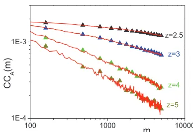
Complementary we introduce a simple stochastic model containing only the information of the laminar length dis-tribution to simulate the emergence of cross-correlations. We assume a process consisting of two phases defined as follows: i) a stochastic variableξ takes the value 1 in the irregular phase and the value 0 in the laminar phase and ii) the length of the irregular phase is always 1, while the laminar length probability density is a power-law with exponent−z/(z−1),zbeing the exponent in the intermit-tent map of eq. (1). Then we generate an ensemble of real-izations of this process and calculate the cross-correlation functionCCr(m) for this ensemble. Here the indexr in-dicates that the ensemble of trajectories used to calculate this cross-correlation function is generated by the underly-ing random process. Despite the simple form of both, the intermittent dynamics in binary representation and the associated stochastic process, large scale computational efforts (105 trajectories have been propagated for 106 it-erations) are needed to achieve convergence of the long-time behaviour of the cross-correlation function. In fig. 1 we show the results obtained for CCA(m) with A =s, r for z = 2.5,3,4,5. The coloured triangles correspond to A =s, while the red lines toA =r. We observe a very good agreement between the two results for eachz value, providing a strong indication that the key quantity deter-mining the scale properties of the cross-correlation func-tion is indeed the laminar length distribufunc-tion, which is the only quantity shared by the two descriptions.
A geometrical interpretation of the emergence of power-law cross-correlations can be obtained by showing that the ensemble of trajectories generated either by the intermit-tent model of eq. (1) or by the simplified stochastic model
Fig. 1: (Colour on-line) The cross-correlation functionCCA(m)
for the symbolic dynamics generated from the intermittent map of eq. (1) (A=s, triangles) and for the stochastic process de-fined in the text (A=r, red lines) for four different values ofz: z= 2.5 (black),z= 3 (blue),z= 4 (olive green),z= 5 (dark yellow). For the numerical simulations we used an ensemble of 105trajectories each of length 106.
introduced above, are realizations of a random fractal set. Thus they can be produced by an automaton [15] and they can also be mapped to a scale-free network using the visibility [16], or the recently generalized cross-visibility algorithm [17]. Adopting this point of view, it is nat-ural to expect that two intermittent trajectories (corre-sponding to two different particles) being two different subsets of a random fractal set or of a scale-free network are power-law cross-correlated. In fact these long-range cross-correlations are dictated by the power-law form of the two-point correlation function of the corresponding set (random fractal or scale-free network).
To demonstrate the fractal properties of the ensemble of trajectories of the simplified stochastic model, we employ techniques used for the calculation of the lower entropy dimension (LED) [18] for random fractal sets. LED cor-responds to the “mass dimension” of usual fractal sets (like for example the Cantor set). Thus, a time-series of length L represented by a sequence of binary symbols (0 for laminar phase and 1 for irregular phase in our case) is interpreted as a set of unoccupied (0) and occupied (1) non-overlapping cells of the embedding set2. In a large ensemble of trajectories all of lengthLand generated us-ing a fixed value ofz, one can calculate the mean number of “1”sN(1, L)(averaging over the ensemble) determin-ing the mean number of occupied cells necessary to cover entirely the so defined random fractal set. Notice that the concept of the “random fractal set” establishes only at the level of the ensemble and it is not defined for indi-vidual trajectories. N(1, L)scales with the lengthL of the embedding set as
N(1, L)=sLdF, (3)
where s is a positive constant and dF is the associated fractal LED. To verify that the ensemble of intermittent trajectories defines a random fractal set, we calculate the
2The embedding set is the set ofLcells.
[image:5.595.325.519.80.213.2]F. K. Diakonoset al.
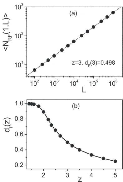
Fig. 2: (a)NRF(1, L)vs. Lfor an ensemble of 106trajectories
generated usingz= 3 and (b) the fractal LEDdF(z)vs. z.
mean number of “1”sN(1, L)for 106 trajectories gener-ated with a fixedz-value and possessing a fixed lengthL. Then we vary the length of the ensemble trajectories from 102to 106calculating for each caseN(1, L). We use the same statistics (106 trajectories) to construct the trajec-tory ensemble for each L-value. In fig. 2(a) we show the result forz= 3 on double logarithmic scale.
We observe a linear behaviour corresponding to a per-fect power-law withdF ≈0.5. This suggests the validity of a general scaling relation of the form
NRF(1, L) ∼LdF(z). (4)
were the fractal LED may depend onz and the indexRF indicates the associated random fractal set. We have per-formed the fractal LED calculation for several values of z in the rangez > 3/2. Our results are summarized in fig. 2(b), where we show the dependence of the fractal LED dF(z) on the exponent of the intermittent dynam-ics z. Notice that the power-laws NRF(1, L) ∼ LdF(z) for different z’s are all of the same quality as measured by the coefficient of determination and the corresponding chi-square per degree of freedom (χ2/dof) of the fit.
Thus, we conclude that the ensemble of the intermit-tent trajectories is equivalent with respect to its com-plexity with a random fractal set with variable dimension dF(z) depending on the characteristic intermittency ex-ponent z. Clearly, the observed fractality refers to the time-dependence, i.e. the considered sets (ensembles of
trajectories) are fractal in time. This geometrical prop-erty makes transparent the existence of cross-correlations among the members of the ensemble. The fractal LED be-comes equal to the embedding dimension forz= 3/2 sig-nalling the absence of long-range cross-correlations in this case. As already mentioned, in the region 3/2 < z < 2 long-range cross-correlations still exist, however there is no clear signal of a power-law form3. This issue requires more extensive studies and it is left for a future detailed study.
Going one step further in our analysis, one can develop a method to find an analytical estima-tion of the cross-correlaestima-tion funcestima-tion CCr(m) based on the above introduced stochastic model. To achieve this, let us first consider two binary se-quences {x(ri)} = {x(1i,r), x(2i,r), . . . , x(k,ri), . . .} and {x(jr)} = {x(1j,r), x2(j,r), . . . , x(n,rj), . . .} generated by the stochastic model. To simplify the notation we will omit the indexrof the trajectory values for the following steps. The function CCr(m) should be proportional to the joint probability Pij(x(ki)= 1;xk(j+)m= 1) that the random variablex(i)has the value 1 at time step k and the random variable x(j) has the value 1 at time stepk+m, averaged over the time
CCr(m) = 1 N−m
N−m
k=1
Pij(x(ki)= 1;x(kj+)m= 1). (5)
Obviously it holds
Pij(x(ki)= 1;x (j)
k+m= 1) =P(x (i)
k = 1)·P(x (j)
k+m= 1) (6) sincex(i)andx(j)are statistically independent. To calcu-lateP(x(ki)= 1) one can use the method introduced in [14] writing
P(x(ki)= 1) = k−1
n=1
P(x(ki−)n= 1)·P1|1(n|x(ki−)n= 1), (7)
where P1|1(n|x(ki−)n = 1) is the conditional probability to have a laminar phase of lengthndirectly after the instant k−n if x(i) has the value 1 at the time instant k−n. The appearance of a laminar phase with duration n is independent of the value ofx(i)at the instantk−n. Thus, we find
P1|1(n|x (i)
k−n = 1) =ρ(n); ρ(n)∼n−
z
z−1; n1, (8)
where ρ(n) is the laminar length distribution normalized to one. Inserting eq. (6) into eq. (5) we obtain
P(x(ki)= 1) = k−1
n=1
P(x(ki−)n= 1)·ρ(n), (9)
which can be solved recursively using as initial condition P(x(1i) = 1) =p0 with p0 ∈(0,1). A similar equation is
3This may be attributed to the fact that the corresponding fractal
[image:6.595.64.261.80.370.2]A universal mechanism for long-range cross-correlations
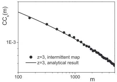
Fig. 3: The cross-correlation functionsCCs(m) (symbolic
dy-namics, intermittent map, black circles) and the analytical es-timation ofCCr(m) (solid line) forz= 3.
obtained also for P(x(kj+)m = 1) replacing simply k with k+m. Having solved eq. (9) one can calculate the left-hand site of eqs. (6), (7) and insert the obtained results in eq. (5) to get an analytical approximation forCCr(m) containing three sums. The validity of the introduced an-alytical scheme is tested in fig. 3, where we show the sym-bolic dynamics resultCCs(m) together with the analytical estimation forCCr(m) usingz= 3.
We observe a very good agreement between the ana-lytical result and the numerical simulations forCCs(m). Notice that numerically calculatedCCr(m) is not shown in this plot. However, as illustrated in fig. 1 the numeri-cal results forCCr(m) andCCs(m) are very close to each other for any considered z and therefore, the analytical estimation of CCr(m) can be also used as an analytical estimation of the cross-correlationCCs(m). The analyti-cal treatment leads us to the conclusion that it is the long-range character of the correlation betweenP(x(ki)= 1) and P(x(kj)= 1) existing for any pair of intermittent trajecto-ries which generates the observed cross-correlations. Note that this property has been discussed in [19] in a different context.
With our analysis we have demonstrated a mechanism to establish power-law cross-correlations between parti-cles which do not interact with each other. This phe-nomenon is induced by the strong intermittent dynamics performed by each of the particles independently. The re-sulting ensemble of trajectories for all particles, despite the absence of a coupling between trajectories of different particles, forms —in a binary representation— a fractal set in time and the underlying self-similarity leads to the establishment of algebraically decaying cross-correlations. Strong intermittency (sporadicity) discussed here is a re-sult of the interaction of a particle with a suitable external potential (field)4. The appearance of long-range cross-correlations deems sporadic dynamics a plausible mecha-nism for the collective behaviour emerging in aN-particle system. Furthermore, since such a collective behaviour
4This could be also a mean field generated by particle-particle
interactions.
is accompanied by scale-free inter-particle correlations, it could be related to the emergence of critical behaviour in the considered system. In fact, a connection of intermit-tent dynamics with criticality has already been established in [20] using the example of the 3D Ising model. There it has been shown that the order parameter fluctuations at the critical point can be efficiently described by an in-termittent map of Pomeau-Manneville type —similar to that of eq. (1)— with additive noise. The exponentz in this intermittent map is related to the isothermal critical exponent δ associated with the second-order transition. This property sets a bound z ≥ 2 necessary for the oc-currence of critical behaviour. It is remarkable that this bound coincides with the bound obtained by our present analysis in order to have a divergent mean laminar length. An astonishing feature of our results is that the power-law cross-correlations emerge even without interaction among the particles. In the context of critical phenomena such a property is welcome, since it could explain universality aspects. Indeed the microscopic interactions between the elementary degrees of freedom of a critical system do not play any role for the determination of the critical expo-nents and the associated scaling laws describing the phe-nomenology of an extended system at the critical point.
In the framework of our approach the obtained correla-tions are determined by the time evolution of the trajecto-ries of two different particles. To enable a closer relation to equilibrium critical phenomena one should extend these ideas also to the case of a field depending both on time and on space. Such an extension requires the use of matrix equations for the field evolution replacing the variablex(ni) by a scalar fieldφ(i, n), whereiis a spatial variable, while n is the time variable. At a first glance one could argue that for the calculation of the spatial cross-correlations one might exchange the role of spatial and temporal vari-ables in the dynamics, use eq. (1) to describe changes of the field φ in space and average over the time variable. This would lead to power-law cross-correlations between the field values at different locations, which is typical for a critical system. However, a consistent treatment of this case requires more elaborate and extensive studies left for future investigations.
∗ ∗ ∗
This work was made possible by the facilities of the Shared Hierarchical Academic Research Comput-ing Network (SHARCNET:www.sharcnet.ca) and Com-pute/Calcul Canada. The authors thank C. Petri and B. Liebchen for fruitful discussions. The per-formed research has been co-financed by the European Union (European Social Fund —ESF) and Greek national funds through the Operational Program “Education and Lifelong Learning” of the National Strategic Reference Framework (NSRF) - Research Funding Program: Her-acleitus II. Investing in knowledge society through the European Social Fund. The authors also thank the IKY and DAAD for financial support in the framework
F. K. Diakonoset al.
of an exchange program between Greece and Germany (IKYDA 2010) and the UK EPSRC for funding under grant EP/E501311/1.
REFERENCES
[1] Samuelsson P., Sukhorukov V. E.andB¨uttiker M., Phys. Rev. Lett.,91(2003) 157002;Cottet A., Belzig W.andBruder C.,Phys. Rev. Lett.,92(2004) 206801; Neder I., Heiblum M., Mahalu D.andUmansky V., Phys. Rev. Lett.,98(2007) 036803.
[2] Yamasaki K., Gozolchiani A. and Havlin S., Phys. Rev. Lett.,100(2008) 228501.
[3] Campillo M.andPaul A.,Science,299(2003) 547.
[4] Laloux L., Cizeau P., Bouchaud J.-P. and Pot-ters M.,Phys. Rev. Lett.,83(1999) 1467; Plerou V., Gopikrishnan P., Rosenow B., Amaral L. A. N.and Stanley H. E.,Phys. Rev. Lett.,83(1999) 1471.
[5] Tumminello M., Aste T., Di Matteo T. and Man-tegna R. N.,Proc. Natl. Acad. Sci. U.S.A.,102(2005)
10421.
[6] Podobnik B.andStanley H. E.,Phys. Rev. Lett.,100
(2008) 084102; Podobnik B., Horvatic D., Petersen A. M.andStanley H. E.,Proc. Natl. Acad. Sci. U.S.A.,
106(2009) 22079.
[7] Takayasu M. and Takayasu H., Statistical Physics and Economics(Cambridge University Press, Cambridge) 2010.
[8] Podobnik B., Wang D., Horvatic D., Grosse I. and Stanley H. E.,EPL,90(2010) 68001.
[9] Cavagna A., Cimarelli A., Giardina A., Parisi I., Santagati R., Stefanini R., Viale F. and Massimil-iano V.,Proc. Natl. Acad. Sci. U.S.A.,107(2010) 11865.
[10] Karlis A. K., Diakonos F. K., Petri C. and
Schmelcher P.,Phys. Rev. Lett.,109(2012) 110601.
[11] Pomeau Y.andManneville P.,Commun. Math. Phys.,
14 (1980) 189; Manneville P. and Pomeau Y., Phys. Lett. A,75 (1979) 1; Hirsch J. E., Huberman B. A.
andScalapino D. J.,Phys. Rev. A,25(1982) 519.
[12] Gaspard P. and Wang X.-J., Proc. Natl. Acad. Sci. U.S.A.,85(1988) 4591.
[13] Schuster H. G.andJust W.,Deterministic Chaos: An Introduction(John Wiley & Sons, Weinheim) 2005. [14] Procaccia I.andSchuster H.,Phys. Rev. A,28(1983)
1210.
[15] Karamanos K.,Kybernetes,38(2009) 1025.
[16] Lacasa L., Luque B., Ballesteros F., Luque J. and Nuno J. C.,Proc. Natl. Acad. Sci. U.S.A., 105(2008)
4972.
[17] Mehraban S., Shirazi A., Zamani M. andJafari G.,
arXiv:1301.1010v1 [physics.data-an] (2013).
[18] Mandelbrot B.,The Fractal Geometry of Nature
(Free-man, San Francisco) 1983.
[19] Izrailev F. M., Krokhin A. A., Makarov N. M.and Usatenko V. O.,Phys. Rev. E,76(2007) 027701.