University of Warwick institutional repository: http://go.warwick.ac.uk/wrap
A Thesis Submitted for the Degree of PhD at the University of Warwick
http://go.warwick.ac.uk/wrap/57673
This thesis is made available online and is protected by original copyright. Please scroll down to view the document itself.
TITLE: Quantifying Finite Range Plasma Turbulence
DATE OF DEPOSIT: . . . .
I agree that this thesis shall be available in accordance with the regulations governing the University of Warwick theses.
I agree that the summary of this thesis may be submitted for publication. Iagreethat the thesis may be photocopied (single copies for study purposes only).
Theses with no restriction on photocopying will also be made available to the British Library for microfilming. The British Library may supply copies to individuals or libraries. subject to a statement from them that the copy is supplied for non-publishing purposes. All copies supplied by the British Library will carry the following statement:
“Attention is drawn to the fact that the copyright of this thesis rests with its author. This copy of the thesis has been supplied on the condition that anyone who consults it is understood to recognise that its copyright rests with its author and that no quotation from the thesis and no information derived from it may be published without the author’s written consent.”
AUTHOR’S SIGNATURE: . . . .
USER’S DECLARATION
1. I undertake not to quote or make use of any information from this thesis without making acknowledgement to the author.
2. I further undertake to allow no-one else to use this thesis while it is in my care.
DATE SIGNATURE ADDRESS
. . . .
. . . .
. . . .
. . . .
Turbulence
by
Ersilia Leonardis
Thesis
Submitted to the University of Warwick
for the degree of
Doctor of Philosophy
Department of Physics
Acknowledgments iv
Declaration and published work v
Abstract viii
Chapter 1 Introduction 1
1.1 Overview of the thesis . . . 1
1.2 The phenomenon of turbulence . . . 2
1.2.1 Introduction: what is turbulence? . . . 2
1.2.2 The turbulence energy cascade . . . 4
1.2.3 HD turbulence and the Kolmogorov 1941 theory . . . . 5
1.2.4 MHD turbulence and the Iroshnikov-Kraichnan model . 10 1.3 Statistical properties of turbulence . . . 12
1.3.1 Intermittency . . . 13
1.3.2 The closure problem and non-Gaussianity . . . 18
1.3.3 Finite range turbulence . . . 19
1.4 The solar corona . . . 21
1.4.1 Introduction . . . 21
1.4.2 Solar magnetic field in the corona . . . 22
1.4.3 Coronal structures and phenomena . . . 25
1.4.4 Solar prominences . . . 27
1.5 Magnetic reconnection . . . 29
1.5.1 Steady reconnection . . . 31
1.5.2 Unsteady reconnection . . . 33
2.1.1 Self-similarity and fractals . . . 39
2.2 Signal processing: deterministic processes and noise . . . 41
2.2.1 Stochastic processes: an overview . . . 42
2.3 Spectral analysis . . . 48
2.4 Probability density function of self-similar processes . . . 52
2.4.1 Normal probability plot . . . 54
2.5 Generalized structure function . . . 54
2.5.1 Extended self-similarity . . . 56
Chapter 3 Hinode/SOT observations of a solar quiescent promi-nence 58 3.1 Introduction . . . 58
3.2 The Hinode mission and the dataset . . . 59
3.3 Analysis of the intensity fluctuations in the time domain . . . 62
3.3.1 Spectral analysis . . . 62
3.3.2 PDF analysis . . . 63
3.4 Analysis of the intensity fluctuations in the space domain . . . 65
3.4.1 Spectral analysis . . . 65
3.4.2 Tests for non-Gaussianity . . . 67
3.4.3 Quantifying the structure function scaling . . . 69
3.4.4 Evidence of the generalized scaling . . . 72
3.5 Conclusions . . . 74
3.5.1 Results summary . . . 74
3.5.2 Discussions . . . 75
Chapter 4 Kinetic PIC simulations of magnetic reconnection 77 4.1 Introduction . . . 77
4.2 2D magnetic reconnection . . . 78
4.2.1 2D reconnection in a symmetric configuration . . . 79
4.2.2 2D reconnection in an asymmetric configuration . . . . 85
4.3 3D magnetic reconnection . . . 94
4.3.1 Coherent structures and scaling laws . . . 95
4.3.2 Intermittent energy dissipation . . . 104
4.4.2 Discussions . . . 108
Chapter 5 Conclusions 110
5.1 Thesis summary . . . 110
5.1.1 Results of the analysis on the Hinode/SOT observations 111
5.1.2 Results of the analysis on the reconnection simulations 112
5.2 Discussions and future work . . . 113
List of Figures 115
List of Tables 118
I acknowledge my supervisor, Prof. Sandra Chapman, for her
supervi-sion during the last four years and especially for giving me the chance to study
one of the most challenging topics in physics: turbulence. During these years I
experienced not only this research field, but also new languages, cultures and
places. I feel I have added a precious piece to the puzzle of my Life.
I would also like to thank my research collaborators and CFSA colleagues,
in particular James, Andy, Nicky and Francisco, for their pleasant company
during my stay here in England.
I am very thankful also to my past and present house mates, in particular
Shyaam, Elena, Natasha, Elizabeth and Giuseppe, for their friendship, which
has contributed to weaken my Italian food and weather nostalgia.
A heartfelt acknowledgement goes to my closest friends, Khurom, Romina
and Chiara, and my relatives, especially my uncle Pino and my cousin-friend
Giuseppe for being always present and concretely helpful.
I am also grateful to my brother Nicola and to my sisters, Giovanna and
Giu-liana, and their partners, Mohamed and Carmelo, “simply” for being part of
my Life. Last, but not least, I am very thankful to my mum and dad, for
giving me freedom and tools to manage and bring value to my Life.
I declare that the work presented in this thesis is my own except where
stated otherwise, and was carried out entirely at the University of Warwick,
during the period of October 2009 to June 2013, under the supervision of Prof.
S. C. Chapman. The research reported here has not been submitted, either
wholly or in part, in this or any other academic institution for admission to a
higher degree. Some parts of the work reported and other work not reported
in this thesis have been published, as listed below:
Publications
• Leonardis, E., Chapman, S. C., Daughton, W., Roytershteyn, V. and Karimabadi, H., Identification of intermittent multi-fractal turbulence
in fully kinetic simulations of magnetic reconnection,Physical Review Letters, 110, 205002, (2013)
• Karimabadi, H., Roytershteyn, V., Wan, M., Matthaeus, W. H., Daughton,
W., Wu, P., Shay, M., Loring, B., Borovsky, J., Leonardis, E., Chap-man, S. C., and Nakamura, T.K.M., Coherent structures, intermittent
turbulence, and dissipation in high-temperature plasmas, Physics of Plasmas, 20, 012303 (2013)
• Chapman, S. C., Nicol, R. M., Leonardis, E., Kiyani, K., and Carbone, V., Observation of Universality in the Generalized Similarity of Evolving
Solar Wind Turbulence as Seen by Ulysses, Astrophysical Journal Letters, 695, L185, (2009)
Conference presentations
• American Geophysical Union (AGU) Fall Meeting, 3-7 December 2012 - San Francisco, California, USA.
Oral presentation: First identification of intermittent turbulence in fully self-consistent kinetic (PIC) simulations of reconnection.
• Magnetosphere, Ionosphere and Solar-Terrestrial (MIST), 30 November 2012 - London, UK.
Poster presentation: First full quantitative characterization of inter-mittent turbulence in 3D particle-in cell (PIC) simulations of magnetic
reconnection.
• American Geophysical Union (AGU) Fall Meeting, 5-9 December 2011 - San Francisco, California, USA.
Poster presentation: Turbulent characteristics of a solar quiescent prominence observed by the SOT on board Hinode.
Poster presentation: Generalized similarity observed in finite range magnetohydrodynamic turbulence in the corona and solar wind.
• Magnetosphere, Ionosphere and Solar-Terrestrial (MIST), 25 November 2011 - London, UK.
• National Astronomy Meeting (NAM), 17-21 April 2011 - Llan-dudno, UK.
Poster presentation: Turbulent characteristics of the intensity fluctu-ations in the Hinode/SOT images of a solar quiescent prominence.
• European Geosciences Union (EGU) General Assembly, 3-8 April 2011 - Vienna, Austria.
Oral presentation: The spatio-temporal characteristics of magneto-hydrodynamic turbulence seen in quiescent solar prominences by
Hin-ode/SOT.
• Magnetosphere, Ionosphere and Solar-Terrestrial (MIST), 26 November 2010 - London, UK.
Poster presentation: Testing for signature of turbulence in Hinode/Solar Optical Telescope (SOT) observations of a solar quiescent prominence.
• HINODE-4: unsolved problems and recent insights, 11-15 Octo-ber 2010 - Mondello, Italy.
Poster presentation: Exploring spatio-temporal turbulent character-istics in solar prominences using the SOT instrument on Hinode.
• Royal Astromonical Society (RAS), 12 March 2010 - London, UK.
Poster presentation: Investigation of universal aspects of evolving MHD turbulence in astrophysical plasmas.
Ersilia Leonardis
Turbulence is a highly linear process ubiquitous in Nature. The
non-linearity is responsible for the coupling of many degrees of freedom leading
to an unpredictable dynamical evolution of a turbulent system. Nevertheless,
experimental observations strongly support the idea that turbulence at small
scales achieves a statistically stationary state. This has motivated scientists
to adopt a statistical approach for the study of turbulence.
In both hydrodynamics (HD) and magnetohydrodynamics (MHD),
fluctua-tions of bulk quantities that describe turbulent flows exhibit the property of
statistical scale invariance, which is a form of self-similarity. For fully evolved
turbulence in an infinite medium, one interesting consequence of this scale
in-variance is the power law dependence of the physical observables of the flow
such that, for instance, the velocity field fluctuations along a given direction
show power law power spectra and multiscaling for the various orders of the
structure function within a certain range of scales, known as the inertial range.
The characterization of such scaling is crucial in turbulence since it would fully
quantify the process itself, distinguishing the latter from a wider class of
scal-ing processes (e.g., stochastic self-similar processes).
Experimentally, it has been observed that turbulent systems exhibit an
ex-tended self-similarity when either turbulence is not completely evolved or the
system has finite size. As consequence of this, the moments of the
struc-ture function exhibit a generalized scaling, which points to a universal feastruc-ture
underling physics of this generalized similarity is still an open question.
This thesis focuses on the quantification of statistical scaling in
turbu-lent systems of finite size. We apply statistical analyses to the spatio-temporal
fluctuations associated with line of sight intensity measurements of a solar
qui-escent prominence and data of the reconnecting fields in simulations of
mag-netic reconnection.
We find that in both environments these fluctuations exhibit the hallmarks of
finite range turbulence. In particular, an extended self-similarity is observed
to hold the inertial range of turbulence, which is consistent with a
general-ized scaling for the structure function. Importantly, this generalgeneral-ized scaling is
found to be multifractal in character as a signature of intermittency in the
tur-bulence cascade. The generalized scaling recovered for finite range turtur-bulence
exhibits dependence on a function, the generalized function, which contains
important information about the bounded turbulent flow such as some
char-acteristics scale of the flow, the crossover from the small scale to the outer
scale of turbulence and perhaps some characteristic features of the boundaries
(future work).
The quantification of the generalized scaling is performed thank to the
appli-cation of statistical tools, some of which have been here introduced for the
first time, which allow to identify the statistical properties of a wide class of
scaling processes. Importantly, these techniques are powerful methodologies
for testing fractal/multifractal scaling in self-similar and quasi self-similar
sys-tems, allowing us to distinguish turbulence from other processes that show
Introduction
1.1
Overview of the thesis
This thesis focuses on the characterization of the inertial range
turbu-lence in systems of finite size by performing statistical methods for the
quan-tification of scaling in self-similar and quasi self-similar processes. We present
analyses of turbulent plasmas in two very different environments, that is, in
the lower solar corona and in simulations of magnetic reconnection.
In the first part of Chapter 1 we give a brief introduction of turbulence
and its phenomenology. We review the statistical approach to the study of
both hydrodynamic (HD) and magnetohydrodynamic (MHD) turbulent flows
along with an overview of its historical development.
In the second part of Chapter 1, we introduce the turbulent systems for which
we present analyses, namely, the solar corona and the magnetic reconnection
process. In particular we highlight the main aspects of such systems which are
relevant for our study.
The statistical techniques used throughout this research work are re-viewed in Chapter 2. Here, we introduce and develop methodologies for
quan-tifying the statistical properties of a wide class of scaling processes. Firstly, we
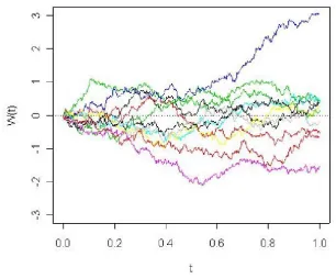
give an overview of few stochastic processes showing self-affinity such as the
Wiener process, the fractional Brownian motion and the Ornstein-Uhlenbeck
process; secondly we focus on a narrower class of scaling processes showing an
extended self-similarity such the turbulent process. We also address
experi-mental issues which may affect the scaling properties of the time/space series
under analysis such as finite size effects of the dataset and noise.
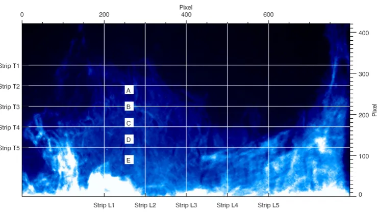
Chapter 3 focuses on the analysis of a solar quiescent prominence in the
lower corona. After a brief explanation on why we have chosen such a system,
we then introduce the Hinode spacecraft which provided the observations for
the analysis. Thus, we apply some of the statistical methods discussed in
Chap-ter 2 to the spatio-temporal intensity fluctuations of the quiescent prominence
under study in order to test whether their statistical properties are consistent
with finite range turbulence.
In Chapter 4 we present the analysis of fully kinetic particle-in-cell
(PIC) simulations of collisionless magnetic reconnection. We analyse the mag-netic field data in the space domain of two reconnection simulations in a
two dimensional (2D) geometry and one reconnection simulation in a
three-dimensional (3D) geometry. Firstly, we focus on the 2D simulations, for which
we consider two cases: a symmetric configuration and an asymmetric
configu-ration of the magnetic field; secondly, we move to the 3D simulation.
In Chapter 5 we present a brief summary of the thesis and the main
results obtained from the analyses of the quiescent prominence seen in Chapter
3 and the PIC simulations of magnetic reconnection seen in Chapter 4. Then,
we conclude by discussing the results focusing mainly on the scaling properties observed to hold the inertial range of turbulence in the two finite sized systems
analysed. Suggestions for future works are also given.
1.2
The phenomenon of turbulence
1.2.1
Introduction: what is turbulence?
The word“turbulence”comes form the Latin word“turba”, which means
disorder. Initially, indeed, turbulence was associated to a chaotic and irregular
motion of people.
During the Age of Renaissance in Italy, Leonardo da Vinci was the first to
apply this term to the apparently random motion of a fluid giving a detailed
description of a turbulent waterfall (see Fig. 1.1). Here, Leonardo highlighted
the important role played by the coherent structures in the flow, such as the
turbu-Figure 1.1: Sketch of a turbulent waterfall made by Leonardo da Vinci.
lent fluid change, the macroscopic characteristics keep organizing themselves in
the same manner every time the phenomenon is reproduced. After Leonardo, many scientists have been interested in this phenomenon, and as many were
the definitions of turbulence proposed. Nevertheless, none of these definitions
has been accepted as a unique, formal and satisfying definition of turbulence.
However, there is consensus on the characteristics shown by turbulent systems
such as the following:
• disorganised, seemingly random behaviour;
• dynamics non-repeatable but statistics repeatable;
• many excited modes/degrees of freedom involved;
• scale-invariance/self-similarity;
• state far from equilibrium;
• enhanced diffusion and dissipation.
The irregularity or random character of all turbulent flows makes a
determinis-tic approach to the turbulence problem nearly intractable. Indeed, even though
the governing equation of fluid dynamics, that is, the Navier-Stokes equation,
[image:16.595.232.410.108.266.2]this equation. Thus, statistical methods have been adopted for the study of fully developed turbulence1, which find their basis on the phenomenological
description of this process.
1.2.2
The turbulence energy cascade
Leonardo’s picture of turbulence gave a considerable contribution to the
understanding of the turbulence phenomenon. As a matter of fact, his view
of turbulence as a process dominated by coherent structures at different scales
laid the foundations, after nearly four centuries, of the well known turbulent
cascade, which establishes the phenomenology of turbulence.
In 1920, Lewis Fry Richardson proposed the first qualitative description of
Figure 1.2: Sketch of the Richardson cascade. (Image from Frisch et al. [1978])
the turbulent cascade [Richardson, 1922]. In his book, Weather Prediction by Numerical Process, he wrote:
‘Big whirls have little whirls that feed on their velocity,
and little whirls have lesser whirls and so on to viscosity.’
Figure 1.2 shows a sketch of the turbulent cascade conjectured by Richard-son. In this model the process of turbulence starts when energy is injected in
the system at large scales l0 and is successively transferred from larger
ed-dies (mother eded-dies) to smaller and smaller eded-dies (daughter eded-dies), until
it dissipates by viscosity at very small scales lη << l0. The input energy is
introduced at the rate ε (per unit mass) which is assumed to be on average
constant throughout the cascade. Also, eddies can have geometries different
to circular and they are space-filling2. Notice that, unlike what is shown in
Figure 1.2, the smaller eddies can also be embedded in the larger eddies.
The scales at which the energy transfer occurs are ln=l0rn, where 0 < r <1
and n is a positive integer. Importantly, these scales establish the so called
inertial range of turbulence and satisfy the following relation lη << ln << l0.
Thus, in a turbulent process, one can distinguish three regions, namely, the
input region, the inertial range and the dissipation region. This embodies the
assumption that, in the inertial range, energy dissipation is not relevant and
the energy transfer takes place locally between two or more structures at close
scales (localness of interactions).
1.2.3
HD turbulence and the Kolmogorov 1941 theory
Let us consider the Navier-Stokes equation for an incompressible, viscid
fluid flow:
∂v
∂t + (v· ∇)v=− 1
ρ∇p+ν∇
2v+f, (1.1)
wherev=v(r, t) is the fluid velocity field at positionrand time t,p=p(r, t) is the pressure field in the fluid, ρ is the density, ν is the kinematic viscosity
and f = f(r, t) is an external force per unit mass doing work on the system. Equation (1.1) expresses the conservation of momentum (Newton’s second law)
and comes along with the mass conservation equation:
∂ρ
∂t + (∇ ·ρv) = 0. (1.2)
2We shall see later in this chapter that both the assumptions of a constant mean transfer
For incompressible fluids, that is, fluids in which the density is constant in both space and time, Equation (1.2) leads to∇ ·v= 0, which is the condition for incompressibility.
We now define the Reynolds number, Re, as the ratio of the non-linear term
and the viscous term of Equation (1.1) and, by applying dimensional analysis,
we obtain:
Re =
|(v· ∇)v| |ν∇2v| =
V2/L νV /L2 =
V L
ν , (1.3)
whereV and Lare respectively some characteristic velocity and length of the
flow. The Reynolds number is a control parameter which indicates whether the flow is laminar or turbulent. It can be shown, indeed, that it is related to
the number of excited degree of freedom of the flow by a dimensional analysis
[Frisch, 1995, p107]. At relatively low Re, a flow can be considered laminar
(few degrees of freedom involved), whilst beyond a certain Re, the many
de-grees of freedom excited interact non-linearly each other and the flow becomes
turbulent. A broad variety of experiments with pipe flows have been made in
order to study the transition from the laminar to the turbulent state of a fluid
[e.g., Van Dyke, 1982; McComb, 1990]. It has been observed that for small
values of the Reynolds number (Re ∼ 1) the flow possesses several
symme-tries, which are consistent with the Navier-Stokes equation (Eqn. (1.1)). As
the Reynolds number increases (Re > 1), these symmetries gradually vanish
and the flow becomes more and more turbulent (see Fig. 1.3). Nevertheless,
at very high Reynolds numbers (Re >> 1), symmetries are restored far from
the boundaries in a statistical sense, leading to a fully developed turbulence3.
If the statistical properties of turbulence at Re >> 1 are also invariant under
translations and rotations in space (or time), then it is referred to as
homoge-neous isotropic fully developed turbulence.
One of the fundamental theories of fully developed HD turbulence was
formulated by Andrey Nikolaevich Kolmogorov in 1941, that is, the so called K41 theory. In the K41 theory, Kolmogorov makes the assumption of locally
isotropic time-steady homogeneous fluid turbulence. The time-steady
condi-tion implies that the energy rate injected into the system, the energy transfer
3In the limit ofR
e−→ ∞the flow becomes chaotic [Frisch, 1995, p8]. However, we shall
Figure 1.3: Schematic view of pipe flow experiments of turbulence at different Reynolds numbers. Notice that turbulence is fully developed for Reynolds numbers larger than 104. (Image from Bohr et al. [1998], p4)
rate and the energy dissipation rate must all be equal on average, while the
local isotropy only holds for very large Reynolds and arises from the fact that
the properties of well developed turbulence at small scales are independent
of the details of the large scales. This has several implications, of which the
most important is that for small scales, or large wave numbers, the turbulence
exhibits universal behaviours.
Let us consider a turbulent flow with the above assumption, then define
the longitudinal velocity increment as follows [Frisch, 1995, p57]
δvk(r,l)≡[v(r+l)−v(r)]· l
l. (1.4)
Kolmogorov thus stated that, in the limit of infinite Reynolds numbers, the
and there exists a scaling exponenth∈ < such that
δv(r, λl)law= λhδv(r,l), ∀λ∈ <+, (1.5)
for allr and increments λl small compared to the integral scale. Under a fur-ther assumption, known as the Kolmogorov’s second universality assumption,
in the limit of infinite Reynolds numbers the statistical properties of δv(r,l) at small scales must depend only on the scale l and mean energy dissipation rate per unit mass ε. Hence, Kolmogorov derived the two-thirds law for the
second moment of the velocity increments as follows
<(δv(l))2 >=Cε2/3l2/3, (1.6)
where C is a universal dimensionless constant4. Notice that Equation (1.6) implies thath= 1/3. Equation (1.6) also implies another important law, that
is, the celebrated five-thirds law for the energy spectrum:
E(k) = CKolε2/3k−5/3, (1.7)
where CKol is a dimensionless constant called the Kolmogorov constant.
Ac-tually, this law was first derived by Obukhov [1941] and, according to Kol-mogorov, was developed independently from the two thirds law [KolKol-mogorov,
1941].
The two thirds and the five-thirds laws have found many confirmations in both
observations and numerical simulations of fully developed turbulence in fluid
flows. However, the main result of the K41 theory is the four-fifths law, which
is one of the few exact and non trivial results in turbulence. Given the third
order structure function of the longitudinal velocity increment, the four-fifths
law establishes the following equality
<(δvk(r,l))3 >=−
4
5εl. (1.8)
Equation (1.8) arises from a dimensionless analysis consistent with the
sim-4In the next section we shall see that the universality of the constantC was soon
ilarity hypothesis of the K41 theory and implies that the rescaling exponent h of the velocity increments in Equation (1.5) must be 1/3. Note also that,
in order to show that h = 1/3, the assumption of isotropy is not necessary
[Frisch, 1995, p89].
Let us now examine the consequences of the K41 theory for the pth
moment of the velocity increments, Sp(l), at the inertial scales l, assuming
homogeneity and isotropy. We define the structure function of order p > 0
along a given direction r, as follows
Sp(l)≡< v(r+l)−v(r)p >=< δv(r,l)p >, (1.9)
where the angular brackets indicate an ensemble average overr. Then, the
two-thirds (Eqn. (1.6)) and the four-fifths (Eqn. (1.8)) laws suggest the following
scaling for thepth order structure function
Sp(l) = Cpεζ(p)lζ(p), (1.10)
where the Cp are dimensionless coefficients and the scaling exponent ζ(p) =
p/3. Notice that, for p = 3, Equation (1.9) leads to the four-fifths law with
C3 = −4/5. Moreover, as stated in the K41 theory, the moment scaling law
only depends on the mean energy dissipation rate ε and the scale l and does
not involve the integral (large) scale l0. Thus, for positive fixed values of
ε, either when ν −→ 0 and/or l0 −→ ∞, the pth moment of the structure
function does not diverge to infinity.
The universal role played by the Cp coefficients has been largely
dis-cussed by the turbulence community. In 1942 Landau pointed out that there
is no reason to suppose the Cp are universal (except for p = 3). Indeed,
ac-cording to Landau, the energy dissipation rate changes over times of the order
of the periods of the large eddies (wl0), therefore the mean energy dissipation
rate ε must depend on the large scales l0 at which the turbulence mechanism
is produced [Landau and Lifshitz, 1987]. As a consequence of this, the Cp
cannot be universal since they are different for different flows (e.g., different
1.2.4
MHD turbulence and the Iroshnikov-Kraichnan
model
The general equations describing an electrically conducting magnetized
flow in the limits of the MHD approximation are the following:
ρ
∂v
∂t + (v· ∇)v
=−∇p+J×B (Momentum conservation) (1.11)
∂ρ
∂t + (∇ ·ρv) = 0 (Mass conservation) (1.12)
∇ ×E=−∂B
∂t (Faraday
0
s law) (1.13)
∇ ×B=µJ (Amp`ere0s law) (1.14)
∇ ·B= 0 (Gauss0law) (1.15)
E+v×B= J
σ (Ohm
0
s law) (1.16)
whereJ is the current density,Bis the induction (commonly called “magnetic field”), E is the electric field, µ is the magnetic permeability and σ is the electrical conductivity. The last four equations in the system above are the
well known Maxwell’s equations. The above system of equations is closed by
an equation of state, which relates the plasma pressure to the temperature
and density, and its form depends on the assumptions that one makes about the thermodynamic state of the systems.
Manipulating the above equations, an expression for the induction can be
derived and written as follows:
∂B
∂t =∇ ×(v×B) +λ∇
2B, (1.17)
whereλ= (µσ)−1is the magnetic diffusivity, which is here considered uniform. As in HD, turbulence arises from the non-linear terms so that, similar to
the usual Reynolds number, a magnetic Reynolds number,Rm, can be defined
as the ratio of the non-linear term and the diffusion term of Equation (1.17),
then
Rm =
V L
λ , (1.18)
the Alfv´en velocity, VA =B/ √
µρ, leading to the definition of the Lundquist number S instead [Biskamp, 1993, p175]. The latter, indeed, is defined as
VAL/λand, unlike the magnetic Reynolds number, does not give any indication
about the possible turbulent status of a MHD flow. As a matter of fact, high
Lundquist numbers (S >> 1) may simply mean that the resistivity is small,
corresponding even to Rm ∼ 0 for static systems. On the contrary, high
magnetic Reynolds numbers only arise from large fluid velocities generated by
the non-linear dynamics, making therefore the system prone to turbulence.
Likewise in HD, fully developed MHD turbulence is characterized by large
magnetic Reynolds numbers (Rm >>1) for which statistical properties of the
fluctuations show universal behaviour and scaling laws.
In MHD flows, there is often a large-scale background field, B0, which cannot be eliminated by a Galilean transformation. As a consequence of this,
turbulent flows are typically highly anisotropic and therefore the assumption
of isotropy is not always valid as it was for the HD case. Indeed, while
dis-persionless Alfv´en waves propagate either parallel and anti-parallel to B0, in the direction perpendicular to B0, shear perturbations at the Alfv´en speed generate at small scales giving rise (potentially) to turbulence [Biskamp, 1993,
p178]. The effect of the Alfv´en waves is to decrease the energy transfer rate in the turbulent cascade; in other words, a single eddy takes longer (with
re-spect to the HD case), to transfer its energy to one or more smaller eddies
[e.g., Carbone, 1993, and references therein]. This led to refinement of the
Kolmogorov’s theory for its applicability to MHD turbulent flows.
In 1964 Iroshnikov and, one year later, Kraichnan laid the foundations of the
MHD turbulence model [Iroshnikov, 1964; Kraichnan, 1965]. By taking into
account the effects of Alfv´en waves on the turbulent cascade, they derived a
power law for the power spectrum of the form
E(k) =CKol0 (VAε)1/2k−3/2, (1.19)
whereCKol0 is a constant which depends onkB0kand hence on the geometry of the large scales eddies. Importantly, this expression is not dimensionless and
thus profoundly differs fromCKol obtained in the Kolmogorov’s five-thirds law
the inertial scales, the Iroshnikov-Kraichnan spectrum depends also on the large-scale background field. Furthermore, the Iroshnikov-Kraichnan model
for MHD turbulence anticipates moments with scaling exponents ζ(p) =p/4,
thus smaller than p/3 expected by the K41 model. Therefore, according to
this model, if the energy transfer rate is constant, then ζ(4) = 1, in contrast
toζ(3) = 1 obtained from K41.
Although the Iroshnikov-Kraichnan spectrum has been often observed
in MHD turbulent flows like the solar wind, however also the Kolmogorov’s
spectrum predicted for HD turbulence has been observed in this environment,
leading to the conclusion that both types of turbulence may coexist in highly anisotropic MHD flows [Chapman and Hnat, 2007].
Moreover, numerical and analytical studies of incompressible MHD turbulence,
where the cascade is mediated by Alfv´en fluctuations, show that the different
scaling exponents for the power spectra might depend upon the strength of
the turbulence, the strength of the background field, kB0k, and anisotropy. Specifically, it has been observed that introducing anisotropy to MHD models
of turbulence, the power spectrum scales as ∼ k⊥−2 for weak turbulence [e.g. Galtier et al., 2000] and ∼ k−5/3⊥ - i.e. the Kolmogorov spectrum - for strong turbulence [e.g., Higdon, 1984; Goldreich and Sridhar, 1995] with respect to the background magnetic field. In particular, Goldreich and Sridhar [1995] showed
that magnetic and velocity field perturbations only occur perpendicular toB0 leading to the following relationship kk =k
−2/3 ⊥ l
−1/3
0 , where l0 is the outer or
energy injection scale. Considering the turbulence cascade picture, this could
be seen as elongated eddies - i.e. “rope-like” or “sheet-like” structures - along
the direction ofB0.
1.3
Statistical properties of turbulence
The dynamical behaviour of any particular flow variable in either HD or
MHD turbulent systems is highly random due to the large number of degrees of
freedom involved, which are coupled through non-linear interactions.
Mathe-matically, the description of such systems should center on invariant measures;
however, there is no rigorous theory about what measures are strictly invariant
the idea that turbulence at small scales achieves a statistically stationary state. This is the basic motivation for seeking a universal statistical description of
turbulence.
In this sections an overview of the main statistical properties of turbulent flows
is given along with some models that have been developed in order to include
these statistical characteristics into the theory of turbulence.
1.3.1
Intermittency
Both the Kolmorogov theory for HD turbulence and the
Iroshnikov-Kraichnan model for MHD turbulence assume that the energy transfer (or
dissipation) rate ε within the inertial range is on average constant. We have
seen that this leads to a linear scaling exponent ζ(p) in p for the various
moments of the structure function. However, the energy transferred by the eddies at the inertial scales l is actually far from uniform, implying that the
self-similarity property of the velocity fluctuations (see Eqn. (1.5)) at the
in-ertial scales is lost. Experimentally this is seen as a non-linear trend of ζ(p)
with p and as a strongly intermittent, bursty, nature of the fluctuations of
the bulk quantities that describe both HD and MHD turbulent flows. This
phenomenon is known as intermittency.
Intermittent signals are typically dominated by large occasional events and
characterized by heavy tailed probability density functions (PDFs) of their
fluctuations. The bursty nature of a random function f(r) in the space (or time) domain can be quantified via the flatness (or kurtosis K) of the
prob-ability distribution of its increments δf(l) = f(r+l)−f(r) 5. The flatness
estimates the importance of the tails of the distribution and is defined as the
normalised fourth moment of a distribution [Frisch, 1995][p122], namely:
K(l) = <(δf(l))
4 >
<(δf(l))2 >2 (1.20)
For a Gaussian distribution K = 3. An excess kurtosis, k, is usually defined
as k = K −3 in order to set k = 0 for Gaussian distributions. The
func-5Notice we have dropped the space argument r in the increments δf(l) by assuming
tion f(r) is then said to be statistically intermittent if the fluctuations δf(l) have flatness that increases asl goes to smaller and smaller scales. Therefore,
according to this definition, neither self-similar nor Gaussian signals are
inter-mittent. From Equation (1.20) we can clearly see that the expression for the
flatness involves the fourth and second moments of the fluctuations suggesting
that, for intermittent turbulence, even higher order statistics will be subject
to modifications.
In 1962, Kolmogorov and Obukhov refined the K41 theory introducing
intermittency effects in the turbulence cascade of energy [Kolmogorov, 1962;
Obukhov, 1962] formulating the well known Kolmogorov-Obukhov theory of turbulence, in short K-O62. This theory was successively developed in detail
in Monin and Yaglom’s texbook of turbulence [Monin and Yaglom, 1971], in
which the authors introduce a local energy dissipation rate at the scale l, εl,
which is statistically independent on the velocity increments
nondimensional-ized by (lεl)1/3 [Frisch, 1995, p164]. This assumption is known as the “refined
similarity hypothesis”. As a consequence of this, all the scaling laws predicted
by the K41 theory were modified as follows [Lesieur, 2008, p230]:
(Two−thirds law) S2(l)∼< ε >2/3 l2/3
l l0
χ/9
(1.21)
(Five−thirds law) E(k)∼< ε >2/3 k−5/3(kl0)−χ/9
(Moments law) Sp(l)∼< ε p/3
l >l
p/3 ∼< ε >p/3 lp/3
l0 l
χp(p−3)/18
whereχ is a universal constant and l0 is the integral scale of turbulence.
Besides the K-O62 model, numerous models have been developed in or-der to include intermittency effects in the turbulence cascade, some of which
employ a (multi)fractal approach to the statistical description of fully
de-veloped turbulence. The use of the fractal geometry arises from the energy
cascade picture: analogously to a fractal, a single eddy can be seen as a rough
part or a fragmented geometric shape that can be subdivided into parts, the
daughter eddies, each of which is a reduced size of the mother eddy [Seuront
et al., 1999]. When intermittency phenomena occur, not all daughter eddies
are generated producing therefore ‘gaps’ in the hierarchy of cascading eddies
a consequence of this, the eddies are no longer space-filling and the energy dissipation rate within the inertial range depends on scalel 6.
Figure 1.4: Sketch of the turbulent cascade: non-intermittent case (left) and intermittent, mono-fractal case (right). (Image from Seuront et al. [1999])
Frisch et al. [1978] developed one of the first models for intermittent HD turbulence using a fractal approach. This model is called theβ-model and
makes use of an “intermittency parameter”µ= 3−Dh, whereDh is the fractal
dimension of the system [Mandelbrot, 1977]. Thus, by defying β ∈ [0,1] as the fraction of daughter eddies of sizel =l0rn produced, where l0 is the outer
6There are several definitions of intermittency in literature, some of which threat the
scale of turbulence,n is a positive integer andr is typically chosen to be equal to 2 for simplicity7, then β = rµ. For β −→ 1, µ −→ 0 (non-intermittent
case) and for β −→0, µ −→ −∞(intermittent case). Consequently also the structure function scaling exponent,ζ(p), is subject to modification as follows
ζ(p) = µ(1−p/3) + (p/3) [Frisch, 1995, p139].
The β-model was also extended to MHD turbulence by [Ruzmaikin et al.,
1995] and, employing the Iroshnikov-Kraichnan model (§ 1.2.4), it yields the following expression for the structure function scaling exponent ζ(p) =µ(1−
p/4) + (p/4).
However, the phenomenology of turbulent cascades is rather more com-plex and mono-fractal models, like theβ-model, do not take into account how
the activity of turbulence becomes more and more inhomogeneous as we go
to smaller and smaller scales8. Let us explain this with an example. Figure
1.4 shows the phenomenology of the turbulent cascade with (right) and
with-out (left) intermittency effects. The intermittent case here shown refers to a
mono-fractal description of intermittency, such as that used in the β-model.
As we can see, mono-fractal models only consider the case for a daughter eddy
of a fixed size to be generated or not. It does not consider the intermediate
case for which eddies of similar but different sizes can be generated. The latter case would be instead taken into account in a multifractal description of the
turbulent cascade as can be seen in Figure 1.5.
One of the first attempts to describe the turbulent cascade by using a
multifractal approach was made by Parisi, who suggested that fully developed
turbulence possesses only a local scaling invariance, that is, the h exponent
in Equation (1.5) can vary at different points of the fluid [Parisi and Frisch,
1985, p84]. This weaken the assumption of global scale invariance made in the
K41 theory allowing a wider spectrum of continuous values forh. This led to a
multifractal description of fully developed intermittent turbulence. Since then,
many multifractal models were developed, the most important of which are
7r=2 simply means that one mother eddy at scalel generates two daughters at scalel/2. 8From an experimental point of view, mono-fractal models are inadequate to describe
Figure 1.5: Multifractal description of the turbulent cascade: mono-fractal description (left) versus multi-fractal description (right). (Image from Seuront et al. [1999])
the revised β-model by Paladin and Vulpiani [1987], the p-model [Meneveau
and Sreenivasan, 1987] and the She-Leveque model [She and Leveque, 1994].
Although there has been progress in the understanding of the intermittency
phenomenon, however it is still an open question due to the several
controver-sies on how to quantify it.
In this thesis we adopt the multifractal approach for the detection of
1.3.2
The closure problem and non-Gaussianity
Fluid turbulence can be considered as a transition state from a laminar
flow in thermal equilibrium to a state very far from it. Small perturbations to
an initially laminar flow slightly lead the system away from thermal
equilib-rium and can be classically treated via the perturbation theory. In contrast,
fully developed turbulent flows typically involve perturbations which interact non-linearly with many degrees of freedom leading the system very far from
thermal equilibrium. In this case, perturbation theories are no longer
ade-quate. Furthermore, while for systems in or near thermal equilibrium, the
total energy is constant, fluid turbulence is instead highly dissipative.
The coupling of the degrees of freedom arises from the non-linear terms in the
fluid equations and a consequence of this non-linearity is the non-Gaussian
nature of the fluctuations associated with the bulk quantities that describe a
turbulent flow.
Let us focus for instance on the HD case by rewriting the Navier-Stoke
equation (Eqn. (1.1)) in the following symbolic fashion [McComb, 1990, p6]:
L0v =L1vv+L2P, (1.22)
where L0, L1 and L2 are differential operators such that L0 = ∂t∂ −ν∇2
,
L1v = −(v· ∇) and L2 = −∇/ρ. We ignore external forces and also the
vector character of the velocity field for illustrative purposes only. If we now write Equation (1.22) in terms of two-point correlation of the velocity field
< vv >, then we get the following expression:
L0 < vv >=L1 < vvv >+L2 < vP > . (1.23)
Multiplying in turn by vv, vvv, ..., before averaging then one obtains a
hier-archy of moment equations [McComb, 1990, p7]
L0 < vvv >=L1 < vvvv >+L2 < vvP > (1.24)
L0 < vvvv >=L1 < vvvvv >+L2 < vvvP >
and so on. This leads to the well known closure problem, which is a common problem of all non-linear equations and consists in having one more variable
than the actual number of equations needed to solve the system. An important
consequence of the closure problem for turbulence is the non-Gaussian nature
of the probability distribution of the velocity field fluctuations; indeed, while
the statistics of a turbulent velocity field at a fixed point is approximately
Gaussian, the two-point, or in general many-point, statistics are typically
non-Gaussian [McComb, 1990, p165].
Several attempts to solve the closure problem have since been made by making
a closure hypothesis on the four-point correlations [Millionshchikov, 1941] such that
< v4 >∼X< vv >< vv >. (1.25)
However this moment-closure assumption implies a near-Gaussian expansion
for the turbulence statistics, which is also not consistent with observations.
Indeed, experimentally measured PDFs at small scales deviate significantly
from Gaussian, and the deviation tends to amplify as the Reynolds number
increases [e.g., Monin and Yaglom, 1971, and references therein].
1.3.3
Finite range turbulence
Turbulence is characterized by strong correlations between different
length/time scales. This is typically seen as power law scaling arising from
the self-similarity of these correlations [Sornette, 2000]. In real situations, however, scaling holds only approximately and a generalized similarity is
in-stead observed.
In fluid turbulence, it has been seen that either when turbulence is not
completely evolved (low Reynolds number), the dataset size or the Reynolds
number are finite (realistic cases) [Sreenivasan and Bershadskii, 2006] or the
system is bounded [Barenblatt, 2004; Cleve et al., 2005], then symmetries in
the flow are broken, and the similarity is lost. Thus, finite-size corrections to
the scaling laws need to be made [e.g., Grossmann et al., 1994; Dubrulle, 2000;
Bershadskii, 2007].
is no longer valid; indeed, the finite size of the system or parameters implies a finite range of the inertial scales of turbulence for which l . l0. As a
consequence of this, scaling laws at the inertial scales might also depend on
the outer scale of turbulence l0.
We have seen so far that both HD and MHD fully developed
turbu-lence in an infinite medium possess statistical scale invariance at small scales,
which leads to power law scaling of the turbulent fluctuations within the
in-ertial range. One of the main consequences of this scale invariance is seen in
the various structure functions of order p, which are expected to exhibit the
following scaling law:
Sp(l)∼lζ(p), (1.26)
where the scaling exponent ζ(p) is experimentally observed to be a non-linear
function ofp (intermittent turbulence).
Often, when dealing with real turbulent flows, Equation (1.26) is no longer
satisfied and an Extended Self-Similarity (ESS) instead suggests a generalized
scaling for thepth moment of the structure function of the form:
Sp(l)∼G(l)ζ(p), (1.27)
where G(l) is an initially unknown function [e.g., Grossmann et al., 1994;
Bershadskii, 2007; Chapman and Nicol, 2009].
ESS was first introduced by Benzi et al. [1993], who observed the
fol-lowing empirical formula
Sp(l) =Sq(l)ζ(p)/ζ(q) (1.28)
to hold the dissipation region of thek spectrum. Successively, it was observed
to hold the inertial range of turbulence in both systems of infinite and finite
size for which respectively Equation (1.26) and Equation (1.27) are satisfied.
This is simply because the ratio of the logarithm of two orders of the structure
function defined as in Equation (1.26) (or Eq. (1.27)) does not depend on the
functionl (or G(l)) directly.
systems such as the fast solar wind [Carbone et al., 1996; Kiyani et al., 2007; Nicol et al., 2008; Chapman and Nicol, 2009], where it appears to be
insensi-tive to the details of the flow [Chapman et al., 2009], in laboratory simulations
of MHD turbulence [Dudson et al., 2005; Dendy and Chapman, 2006] and in
HD turbulence [Grossmann et al., 1994; Bershadskii, 2007]. Moreover, the
generalized function points to a characteristic feature of a wide class of
scal-ing processes that show ESS [Dubrulle, 2000]; however there are still several
unsolved questions: what does determine its functional form? Is it a universal
function or does it depend on the details of the flow?
In this thesis we do not claim to address all these questions, we rather provide analysis tools for the identification and quantification of the generalized
scal-ing in order to investigate its universal features. We also take advantage of the
compensate for the generalized function to develop new tests for multifractal
intermittent turbulence in real systems.
1.4
The solar corona
1.4.1
Introduction
The atmosphere of the Sun is mainly composed of three layers. From the Sun’s surface outward we find: the photosphere, the chromosphere and
the corona (see Fig. 1.6). Although these three layers are very close to each
other, they are characterized by very different physical parameters. As we can
see in Table 1.1, above the photosphere the temperature is about∼4×10³K
and rises through the chromosphere reaching very high temperatures in the
corona. Here the plasma is highly ionized and extends for hundred of
thou-sands of kilometres into the interplanetary space becoming the solar wind.
The reason why the corona has temperatures 200 times hotter than the
pho-tospheric temperature and especially how these can be maintained is still an open debate. However, it is widely recognized that the coronal heating is
related to the magnetic field’s activity [Kivelson and Russel, 1995, p79].
The solar corona is a very inhomogeneous and tenuous layer of plasma
transparent to photospheric light, and becomes visible only during total solar
Figure 1.6: Sketch of the Sun’s structure. (Image available on line)
Layer Temperature (K) Density (m−3) Thickness (Mm)
Photosphere ∼4×10³ 1023 0.5
Chromosphere ∼104 1017 2.5
Corona ∼105−106 1015−107
-Table 1.1: Characteristic parameters of the three layers of the Sun’s atmo-sphere [Kivelson and Russel, 1995, p61].
comes from the Latin word for crown, to indicate the halo visible during total
solar eclipses (see Fig. 1.7).
In the corona many spectacular as well as energetic phenomena take place.
The observed correlation of the coronal structures’ variability with the solar
cycle led to the conclusion that the coronal dynamics strongly depends on
the solar magnetic field [Golub and Pasachoff, 2010, p87]. Thus, in order to
understand the physics of the corona, a deeper study of the coronal magnetic
field is needed.
1.4.2
Solar magnetic field in the corona
[image:35.595.176.463.107.317.2]there-Figure 1.7: Upper panel: image of the solar corona during a solar eclipse from Mongolia in 2008, when the Sun was at the minimum of its activity. Lower panel: zoom of the image in the upper panel. Bright coronal structures, which outline the coronal magnetic field, are visible above the solar limb in contrast with the dark background. (Images courtesy of Miloslav Druckmuller)
fore particles can only move along the field lines. The latter are of two ty-pologies: close magnetic field lines and open magnetic field lines. Close-field
regions are mainly placed at low solar latitudes forming the so called coronal
loops (see Fig. 1.8). The slow solar wind originates here: the closed field lines
act as a constraint for the coronal plasma flow, whose motion outward the
Sun’s atmosphere into the interplanetary space is therefore slowed down. In
poles9. These regions are also known as coronal holes as they connect the solar surface with the interplanetary field and are the source of the fast solar wind.
Figure 1.8: Image of the solar corona during solar minimum at 171 ˚Angstr¨om taken with the Solar Dynamics Observatory on July 12, 2012. High density hot loops are seen to outline the magnetic filed lines of the corona.
It is possible to distinguish two main regions in the corona: active
regions where the magnetic field is much intense and its force lines appear
very bright in the visible, and quite regions where the field is less intense
and no important phenomena seem to occur. The strongly localized magnetic
field in the active regions generates several magnetic structures and dynamical processes in corona, which are constantly observed by numerous satellites (e.g.,
SoHO, HINODE, STEREO, SDO) and are matter of study for the development
and testing of a broad range of models spanning from the loops oscillations
models to the coronal heating models.
A further distinction between two coronal regions is usually made due
to its non-uniformity: the upper (or outer) corona and the lower corona.
Sci-entists distinguish these two regions because of the different trend of their
physical quantities. In particular, while both the density and magnetic field
decrease with the distance going from the lower to the outer corona, it is found
9This is almost true during solar minimum, however during solar maximum they can be
that the density drops faster in the lower corona and the magnetic field drops faster in the outer corona [Aschwanden, 2004, p204]. Nevertheless, it is quite
difficult to experimentally measure the magnetic field in the corona because of
its strong non-linearity and the complexity. This is thought to be the result
of the coupling between the solar dynamo and the coronal magnetic field [e.g.,
Pinto et al., 2011] and also due to a persisting photospheric turbulence in the
corona [e.g., Abramenko et al., 2008; Dimitropoulou et al., 2009]. Intriguingly,
correlations between outer corona and solar wind have also been found in the
statistics of large-scale density fluctuations [Telloni et al., 2009] suggestive of
a coronal turbulence convected with the solar wind plasma [Matthaeus and Goldstein, 1986].
1.4.3
Coronal structures and phenomena
We have seen so far that coronal structures are dominated by the
so-lar magnetic field. At low latitudes, where the field lines are closed, the most
characteristics coronal structures are the loops, which behave as “highlighters”
of the magnetic field lines.
Over active regions, the white-light corona also shows huge long-lived particle
condensations extending outward the Sun (see Fig. 1.7). These structures
are known as “coronal streamers” and occur mainly at the Sun’s equator.
Among these streamers, more specific structures have been identified as
“hel-met streamers”, which are centered over prominences10 often separating dif-ferent magnetic field polarities. Moving toward the solar poles, within coronal
holes, plumes are visible. These are outgoing flows similar to jets, which move
along the open magnetic field lines and have a lifetime of about 24 hours.
Even though the large-scale coronal structures mentioned above have clear
characteristics, however during the maximum of the solar activity they are no
longer distinguishable from each other (see Fig. 1.9).
Besides the structures that characterize the corona, the latter is also
dominated by large-scale erupting phenomena that can occur suddenly
through-out the Sun’s atmosphere. These phenomena are commonly associated with bursting events or explosions by which the corona expels X-ray, energy and/or
Figure 1.9: Image of the solar corona taken at Clifton Beach during a total solar eclipse in 2012, when the Sun was at the maximum of its activity. (Image courtesy of Wendy Vysma-Gooch and Tony Surma-Hawes)
matter. The former are known as X-ray bursts, while explosions with a
subse-quent release of energy and/or matter are called respectively flares and
Coro-nal Mass Ejections (CMEs). These three phenomena are often observed to
occur simultaneously, however they may also take place independently. In
any case, they are strongly related to the coronal magnetic field. Indeed, a
change in the magnetic field line configuration determines a restructuring of the coronal structure and a release of energy under the form of accelerated
flow, energetic particles and X-ray emission trough the magnetic reconnection
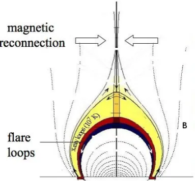
process11. Figure 1.10, for instance, shows the standard 2D model for flares
originally developed by Carmichael and Sturrock [Carmichael, 1964; Sturrock,
1966] and successively re-elaborated by Shibata and Tsuneta [Shibata, 1995;
Tsuneta, 1996]. According this model, flares originate in active regions such
as prominences, where an initial driver causes the prominence to rise with a
consequent transition of the magnetic field from an equilibrium state to a non
equilibrium state. Then, the rising prominence stretches generating a current sheet, which is prone to Sweet-Parker or Petschek reconnection.
Figure 1.10: Standard 2D model for flares.
1.4.4
Solar prominences
Solar prominences or filaments are relatively cool, dense plasma
struc-tures in the lower solar corona with temperastruc-tures of about 104 K. Solar
fil-aments can be seen on the disk, whilst prominences are observed above the
solar limb (see Fig. 1.11). In practice, they are classified in three main
cat-egories according to their location on the Sun, namely active, intermediate and quiescent. The latter usually occur on the quiet Sun at high latitudes
and consequently are also known as “polar crown” prominences, while
ac-tive and intermediate filaments are often observed at low latitudes associated
with active regions [Engvold, 1998]. All prominences originate from filament
channels and develop above the polarity inversion line showing many
differ-ent morphologies and dynamics [see Mackay et al., 2010, for a recdiffer-ent review].
In particular, some observations of filaments on the disk show that they are
mainly composed of thin horizontal threads [e.g., Zirker et al., 1998; Lin et al.,
2005], while others show vertically striated prominences often associated with up and down flows [e.g., Engvold, 1981; Martres et al., 1981]. There is as yet
reach coronal heights and maintain there, suspended against gravitational free fall.
Figure 1.11: Images of the Sun taken by SDO on August, 2012 showing a solar prominence (left) and a filament (right), which is nothing else than the same structure seen on the solar surface three days later after the Sun rotation.
Many models have been developed to describe possible scenarios for the
production and maintenance of such dynamical structures in the corona and
the local magnetic field is suggested to play a key role as it is thought to be the
driver of the prominence threads [e.g., Low and Hundhausen, 1995; Foullon et al., 2009; Hershaw et al., 2011]. Recently, in strongly inhomogeneous
coro-nal plasma structures, processes such as magneto-thermal convection in solar
prominences [Berger et al., 2011] and Kelvin-Helmholtz instabilities in the
corona [Foullon et al., 2011] have been suggested as mechanisms for the
gener-ation of such dynamical structures. In particular, Berger et al. [2010] showed
that quiescent prominences (QPs) often exhibit highly variable dynamics
char-acterized by several up-flows and vortices suggestive of turbulence. The latter,
indeed, could be the reason for the continuous formation process of QPs.
In Chapter 3 we shall test this idea by applying statistical analyses to one of the QPs discussed in Berger et al. [2010] in order to detect and quantify its
1.5
Magnetic reconnection
Magnetic reconnection is an ubiquitous process in both astrophysical
and laboratory plasmas. Experimentally it has been observed that driven
plasmas can show changes in their magnetic field topology along with a release
of energy [e.g., Dungey, 1961; Dere, 1996; Browning et al., 2008]. One of the
main proposed mechanisms for the change of the magnetic field topology is
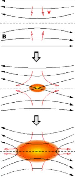
magnetic reconnection. During this process, two oppositely directed magnetic
field lines approach each other, stretch, then break and reconnect changing their topology (see Fig. 1.12); consequently, the magnetic field energy stored
in the force lines is released and rapidly converted into thermal and kinetic
[image:42.595.255.383.337.639.2]energy [Priest and Forbes, 2000, and references therein].
For an ideal MHD flow, for which the resistive term J/œ is negligible compared to the other terms in Equation (1.16), the induction equation (Eqn.
(1.17)) reduces to the following expression:
∂B
∂t =∇ ×(v×B), (1.29)
where the term λ∇2B has been neglected for finite values of the resistivity
η = 1/σ = λµ, in the MHD limit of large length scales (L −→ ∞). As a consequence of this, the magnetic lines of force are ‘frozen-in’ and move with
the flow, therefore a change of the magnetic field topology is not permitted
because it would require a change of the magnetic flux within the frame of the
plasma. This is also known as the Alfv´en’s theorem.
However, magnetic reconnection processes have been observed to take place
in many astrophysical environments (e.g., magnetospheres, solar flares) and laboratory experiments (e.g., tokamaks) in which the plasma can be considered
quasi-ideal [Yamada et al., 2010]. In these systems, indeed, current sheets of
finite size (L small) generate, which invalidates the MHD limit leading to the
break down of the Alfv´en’s theorem. Hence, the ideal MHD description of
the reconnection process is not adequate and models using the Hall MHD,
two-fluid or the Vlasov theory are needed.
The electromagnetic energy released during a the reconnection process
can be derived by using the Ohm’s law (Eqn. (1.16)). Manipulating this
equation we get the following expression:
E·J =−v·(J×B) + J
2
σ . (1.30)
For a steady state (∇ ×E) = 0, therefore we can write the term on the l.h.s. of Equation (1.30) as follows:
E·J=−∇ ·(E×H), (1.31)
whereH=B/µ and∇ ·(E×H) is the Poynting flux, which expresses the rate of inflow of electromagnetic energy per unit area. Thus combining Equations
(1.30) and (1.31) and integrating over the diffusion region, we can deduce that
and work done by the Lorentz forceJ×B. Reconnection is thus a mechanism which both accelerates particles and thermally heats the plasma.
A time-scale for magnetic dissipation, τd, can be obtained from the induction
equation (Eqn. (1.17)) by equating the magnetic time derivative and the
dissipation term (second term on the r.h.s.), leading to the following expression
τd = L2µ/η. However, estimations of the dissipation time in real systems
where reconnection occurs (e.g., in the magnetosphere, solar flares, CME, etc)
are inconsistent with such expression as this phenomenon is observed to take
place much faster. This inconsistency has led many physicists to develop
several models, which can be divided in two main categories: models for steady reconnection and models for unsteady reconnection.
1.5.1
Steady reconnection
The first qualitative model of reconnection was formulated by Parker
[1957] and Sweet [1958]. This model employs a 2D steady state MHD
descrip-tion of the reconnecdescrip-tion process which occurs in a small area within the current
layer, that is, the diffusion region of length 2L and width 2l (see Fig. 1.13).
During this process, the plasma flows into the dissipation region at a speed
vi, the inflow speed, and leaves at speed vo, the outflow speed. Conservation
of mass then implies that Lvi =lvo. Since the magnetic force accelerates the
plasma to the Alfv´en speed, VA, then it can be demonstrated that vo ≈ VA
at the inflow. Then the Sweet-Parker model anticipates a reconnection rate, vi/vo, proportional to S−1/2, where S ∼ LVA/λ is the Lundquist number at
the inflow. Therefore, the larger is L the slower is the reconnection process.
In astrophysical environments where reconnection takes place, such as solar
flares, L is normally large, while λ is thought to be very small; hence, the
release of magnetic energy would be expected to occur in a time of the order
of 107 years [Giovanelli, 1946]. On the contrary, experimentally, this time has
been observed to be few Alfv´en time scalestA=L/VA, thus much faster than
the time anticipated by the Sweet-Parker model.
In 1964, Petschek proposed a new theoretical MHD model for 2D re-connection. This model anticipates the presence of standing-slow mode waves,
Figure 1.13: Sweet-Parker reconnection. The shaded rectangle represents the diffusion region, while the black arrows indicate the inflow (thick) and the outflow (thin) plasma velocity.
magnetic energy into kinetic energy [Petschek, 1964]. Importantly, this model
assumes that the diffusion region is not equal to the global scale 2L, as in the
Sweet and Parker model, but it is limited to a small segment (localized resis-tivity). As a consequence of this, the reconnection ratevi/vo is proportional to
1/log(S); sincelog(S) varies slowly, then the reconnection rate is much larger
than the Sweet-Parker rate, allowing the process to proceed much faster. Since
then, it is referred to such process as “fast magnetic reconnection”, for which
rates typically range between 0.01 and 0.1.
Although the Petschek model was accepted for several years, however it lacks
of an appropriate treatment of the diffusion region; indeed, Petschek’s solution
in the outer region is correct and stable, but it does not match to the diffusion
layer for small η. Thus, numerous modifications to the Petschek model were formulated (i.e. Petschek-like models of fast reconnection), which make use
of an “anomalous” resistivity, ηX =O(1), that is, a locally strong resistivity
in proximity of the X-point [Biskamp, 1993, p137]. Drake et al. [2006] also
proposed that the Hall electric field along with whistler waves are required in
order to set up the original Petschek scheme: the dispersive properties of the
whistler waves permit the flux of electron through the inner diffusion region to
remain finite, even as the dissipation approaches zero. However, rates
consis-tent with fast reconnection have been shown either without employing the Hall
plasmas in absence of whistler waves [Bessho and Bhattacharjee, 2005]. Hence, determining whether the resistivity is either uniform (Sweet-Parker model) or
localized (Petschek model) is crucial to fully understand the dynamics of the
dissipation region and therefore to model the reconnection process.
Recently, high performance supercomputers have allowed deeper
stud-ies of the reconnection process via numerical simulations spanning from MHD
to kinetic regimes. These simulations have shown that for Lundquist numbers
greater than a critical value, Scrit ∼ 104, the initial current sheet becomes
unstable giving rise to instabilities [Loureiro et al., 2007; Lapenta, 2008;
Bhat-tacharjee et al., 2009; Daughton et al., 2009; Huang and BhatBhat-tacharjee, 2010]. Then, the hypothesis of a time-dependent scenario have arisen, which will be
discussed in the next section.
1.5.2
Unsteady reconnection
As larger kinetic simulations became possible, one interesting result was
that magnetic reconnection evolves non-linearly becoming unstable to
plas-moids [e.g. Daughton et al., 2006; Shay et al., 2007, and references therein].
Diffusion processes can drive three different types of resistive instabilities:
gravitational, rippling, and tearing mode [Furth et al., 1963].
In particular, tearing instabilities may occur during reconnection processes
within current sheets whose thickness satisfies the following relation td tA;
consequently, magnetic structures such as islands in 2D (see Fig. 1.14) or flux ropes in 3D, generate while magnetic energy is released.
Secondary tearing instabilities have also been observed in a variety of
2D kinetic simulations of reconnection, which have shown that electron-scale
current sheets become unstable to the formation of magnetic structures on
multiple scales [Daughton et al., 2006; Drake et al., 2006; Karimabadi et al.,
2007; Klimas et al., 2008]. This has led to the so called “fragmentation
pro-cess” [B´arta et al., 2010], for which the current sheet is fragmented to smaller
and smaller plasmoids trough tearing instabilities (see Fig. 1.15). Besides this
“plasmoid instability” [Loureiro et al., 2007; Uzdensky et al., 2010], also called “cascading reconnection” [Shibata and Tanuma, 2001], an inverse cascade


![Table 1.1: Characteristic parameters of the three layers of the Sun’s atmo-sphere [Kivelson and Russel, 1995, p61].](https://thumb-us.123doks.com/thumbv2/123dok_us/9607843.463773/35.595.176.463.107.317/table-characteristic-parameters-layers-sun-sphere-kivelson-russel.webp)