Enhancing nano scale computational fluid dynamics with molecular pre simulations : unsteady problems and design optimisation

http://wrap.warwick.ac.uk

Original citation:

Holland, David M., Borg, Matthew K., Lockerby, Duncan A. and Reese, Jason M.. (2015)

Enhancing nano-scale computational fluid dynamics with molecular pre-simulations :

unsteady problems and design optimisation. Computers & Fluids, Volume 115 . pp.

46-53. ISSN 0045-7930

Permanent WRAP url:

http://wrap.warwick.ac.uk/67260

Copyright and reuse:

The Warwick Research Archive Portal (WRAP) makes this work of researchers of the

University of Warwick available open access under the following conditions.

This article is made available under the Creative Commons Attribution 4.0 International

license (CC BY 4.0) and may be reused according to the conditions of the license. For

more details see:

http://creativecommons.org/licenses/by/4.0/

A note on versions:

The version presented in WRAP is the published version, or, version of record, and may

be cited as it appears here.

Enhancing nano-scale computational fluid dynamics with molecular

pre-simulations: Unsteady problems and design optimisation

David M. Holland

a

_{, Matthew K. Borg}

b

_{, Duncan A. Lockerby}

a,⇑

_{, Jason M. Reese}

c

a

School of Engineering, University of Warwick, Coventry CV4 7AL, United Kingdom

b

Department of Mechanical & Aerospace Engineering, University of Strathclyde, Glasgow G1 1XJ, United Kingdom

c

School of Engineering, University of Edinburgh, Edinburgh EH9 3JL, United Kingdom

a r t i c l e

i n f o

Article history:

Received 31 December 2014

Received in revised form 27 February 2015 Accepted 26 March 2015

Available online 1 April 2015

Keywords: Nanofluidics

Computational fluid dynamics Molecular dynamics Hybrid methods Design optimisation Murray’s Law

a b s t r a c t

We demonstrate that a computational fluid dynamics (CFD) model enhanced with molecular-level infor-mation can accurately predict unsteady nano-scale flows in non-trivial geometries, while being efficient enough to be used for design optimisation. We first consider a converging–diverging nano-scale channel driven by a time-varying body force. The time-dependent mass flow rate predicted by our enhanced CFD agrees well with a full molecular dynamics (MD) simulation of the same configuration, and is achieved at a fraction of the computational cost. Conventional CFD predictions of the same case are wholly inade-quate. We then demonstrate the application of enhanced CFD as a design optimisation tool on a bifurcat-ing two-dimensional channel, with the target of maximisbifurcat-ing mass flow rate for a fixed total volume and applied pressure. At macro scales the optimised geometry agrees well with Murray’s Law for optimal branching of vascular networks; however, at nanoscales, the optimum result deviates from Murray’s Law, and a corrected equation is presented.

Ó2015 The Authors. Published by Elsevier Ltd. This is an open access article under the CC BY license (http:// creativecommons.org/licenses/by/4.0/).

1. Introduction

Many emerging applications of nanofluidic technology take advantage of different physical effects that dominate at small scales; examples can be found in air and water purification[1,2], and in micro chemical reactors[3,4]. The design of these technolo-gies would be greatly facilitated by being able to perform numeri-cal simulations that predict mass flow rates and heat transfer. Computational fluid dynamics (CFD) is regularly used to model and create optimal every-day engineering designs efficiently. However, the assumptions used to derive the continuum fluid equations become invalid in highly-confined systems, making the equations inaccurate. On the other hand, molecular dynamics (MD) can be used to perform highly detailed simulations of nano-scale systems; it has been successfully used to study the behaviour of protein folding[5], crystal formation[6]and chemical reactions[7]. The drawback is that MD is extremely computation-ally intensive, especicomputation-ally when used to model systems comprising hundreds of thousands of molecules that would be required for engineering applications.

The continuum fluid assumptions become inaccurate for gas flows as the smallest characteristic scale of the geometry (e.g.

channel height) approaches the mean distance between molecular collisions (i.e. the mean free path)[8]. When modelling dense liq-uids (as we do in this paper) there is not a well-defined condition for when the fluid assumptions become inaccurate. However, it appears that they fail when water is confined in channels of width

1–2 nm (see [9] and references therein), and MD simulations have been used to show that Lennard-Jones fluids confined in geometries of2–3 nm still show continuum behaviour[10–12]. At the nano-scale the fluid molecules form layers parallel to an interface, which causes the strain rate to vary rapidly within sev-eral molecular diameters [13]. These large variations mean the stress no longer has local linear behaviour[14,15].

Despite the complexities of fluid behaviour at the nano-scale, it has recently been shown that useful predictions from CFD can be obtained for some simple geometries, if appropriate fluid state models, viscosity relationships, and slip models are extracted from an MD pre-simulation[16]. In[17], a similar approach is used to obtain CFD predictions of flow through a nanotube; with results agreeing well with full MD simulations.

However, what remains to be tested is the robustness of nano-scale CFD when applied to more complex engineering calculations. In this paper, we test if our enhanced CFD model is robust enough to predict flow behaviour in a non-trivial geometry (a converging– diverging channel), while using various forms of applied forcing to generate unsteadiness within it. As a demonstration of its

http://dx.doi.org/10.1016/j.compfluid.2015.03.023 0045-7930/Ó2015 The Authors. Published by Elsevier Ltd.

This is an open access article under the CC BY license (http://creativecommons.org/licenses/by/4.0/). ⇑Corresponding author.

E-mail address:[email protected](D.A. Lockerby).

Contents lists available atScienceDirect

Computers & Fluids

efficiency, we go on to apply the enhanced CFD to the design opti-misation of a small fluidic network.

The paper is structured as follows. In the next section we sum-marise the MD pre-simulation procedure and the CFD model used. We then use these models to perform unsteady simulations of a converging–diverging channel, where the width of the channel is close to the continuum limit. Our model is then applied to simulate an industrially-relevant problem of flow through a bifurcating channel. We show that to optimally design the channels the slip velocity at walls must be taken into account. The paper then ends with a summary.

2. Methodology

2.1. The MD pre-simulations

As in [16], we employ preliminary molecular dynamics (MD) simulations to obtain fluid properties and boundary conditions that enable the effective use of a Navier–Stokes fluid solver for nano-scale applications. This approach can be classed as a ‘‘sequen-tial molecular-continuum hybrid method’’ (see[18]for a review of hybrid methods), where ‘sequential’ refers to the fact that the MD is performed in advance of, and so independent of, the continuum-fluid solver.

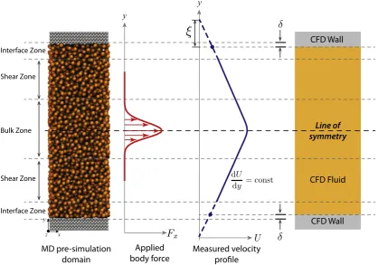
Fig. 1 (far left) shows a schematic of the MD pre-simulation domain; it is symmetrical about its centrelines and uses periodic boundary conditions in the streamwise direction (in thex -direc-tion) and into the page (in thez-direction). The domain hasbulk,

shearand interface zones (as labelled) for measuring state, con-stitutive and boundary properties, respectively. Pressure and den-sity are measured in the bulk zone. In addition to this, in the bulk zone an artificial streamwise body forceðFxÞis applied (Fig. 1, cen-tre left), which creates a velocity profile in the domain similar to that illustrated (Fig. 1, centre right). We assume that the equation

of state in the bulk zone is unaffected by the magnitude of strain rate generated. In the shear zone the fluid is, therefore, subject to a constant shear stress,

s

xy, directly resulting from the bulk-zone forcing. A linear flow velocity profile is developed in the shear zone, and this is least-squares fitted to obtain a strain rate and shear viscosity coefficient,

l

.

Any significant density oscillations associated with molecular layering are confined to the interface zone. In this zone we calcu-late what we term the ‘CFD surface displacement’,d, which is the distance that a CFD wall/surface needs to be displaced from the centres of surface atoms in order to accurately represent the boundary of the fluid (as opposed to the boundary of the solid); seedinFig. 1. We take this displacement to be the distance from the centre of the surface wall atoms to where the fluid density becomes at least 10% of the bulk, i.e.

q

Pa

q

bulk, where a¼0:1. Note, the surface displacement is quite insensitive to the percent-age of the bulk density chosen as the threshold, since the density increases from zero to well above the bulk density over a very short distance. For example, had we chosen the threshold to be at 20% of the bulk density, the surface displacement would have only been 1–2% larger, for a typical case.

The linear velocity profile obtained in the shear zone is extrapo-lated into the interface zone to find the apparent slip length,n, as defined from the CFD surface (seeFig. 1, centre right).

The molecular dynamics pre-simulations, and the full-scale MD simulations used for benchmarking, are performed using the

mdFoam solver [19–22] that is implemented within the OpenFOAM libraries [23]. For the test cases considered in this paper we have adopted a simple Lennard-Jones (LJ) fluid model (at 292.8 K), where the solid LJ wall atoms are fixed/frozen [24]. However, the methodology is general to any given molecular model. For full details of the molecular pre-simulation domain and the molecular dynamics parameters used, the reader is referred to[16].

MD pre-simulation

domain

Applied

body force

CFD Wall

CFD Wall

CFD Fluid

Measured velocity

pr

Interface Zone Shear Zone Bulk Zone Shear Zone Interface Zone

[image:3.595.93.512.446.739.2]

Line of

symmetry

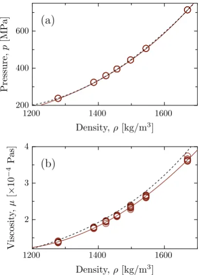
Fig. 2(a) shows MD pre-simulation measurements of pressure, obtained from the standard Irving–Kirkwood expression[25], vary-ing with the mass density. The MD pre-simulation results are least-squares-fitted to a 2nd order polynomial. This then serves as an equation of state within the enhanced CFD solver to connect the mass continuity equation to the momentum equation. In this case the polynomial isp¼0:001559

q

2_3:387

_q

_þ2020:6.

The strain-rate is extracted from the MD shear zone by a least-squares linear fit to the relaxed and time-averaged velocity profile. The applied shear stress is measured using the Irving–Kirkwood equation, from which we obtain a dynamic shear viscosity cient for the LJ fluid at a given bulk density. The viscosity coeffi-cients measured from our MD pre-simulations of Lennard-Jones argon are shown in Fig. 2(b). A least-squares polynomial fit of 2nd order in density is also plotted:

l

¼7:961010

q

2_1:774106

_q

þ0:001106. This is then used in our enhanced CFD simulations to close the momentum equation. Note, due to the breakdown of the continuum assumption and the existence of non-local stress, this state-dependent viscosity becomes only approxi-mate when applied to a nano-confined fluid.

The surface displacement d defines the location of the CFD boundaries relative to the atomic (actual) walls. Ifdvaries substan-tially with density (or any other fluid property), the geometry of the enhanced CFD domain becomes dependent on the CFD solution itself. However, for the fluid/solid combination considered in this paper, over the density ranges considered,dis effectively constant, as seen inFig. 3.

In certain cases the value ofdwill itself be dependent on the geometry, particularly for high curvatures, such as around sharp corners and obstructions. It is beyond the scope of the current work to attempt to accommodate these influences, while noting that, later, we obtain good agreement with full MD simulations

without doing so. To tackle geometry-dependent flow properties (including surface displacement) would dramatically increase the parameter space that the pre-simulations would be required to supply information for; in fact, for such problems a ‘concurrent’ hybrid approach is likely to be more efficient.

As the spatial-scale of the geometry increases, the relative sig-nificance of the surface displacement reduces. We can develop a simple gauge of its impact by considering the percentage that it modifies the mass flow rate in a simple channel in two limiting cases: assuming no-slip at the walls (i.e.n¼0); and for very high slip (i.e.nh, wherehis the channel width). In the no-slip case, for Poiseuille flow, the mass flow rate is proportional to the cube of the channel width; the percentage difference of using the sur-face displacement is then

¼ 1ðh2dÞ

3

h3 !

100%: ð1Þ

For the cases in Section3, where the channel width varies,

is28– 44%. For high-slip cases, where the velocity profile becomes plug-like, the mass flow rate becomes proportional to the square of the channel width, giving a percentage difference:

¼ 1ðh2dÞ

2

h2 !

100%: ð2Þ

Considering again the cases in Section3,

would be20–32%; i.e. the impact of the surface displacement is likely to be very signifi-cant regardless of the degree of velocity slip. Based on the estimates of Eqs.(1) and (2), the impact of a surface displacementd0:2 nm will only be less than 1% (i.e. negligible) for channels greater than 75–100 nm.

Liquid slip velocity at surfaces is calculated using the Navier slip condition:

uslip¼n

c

_; ð3Þ

wherenis the slip-length and

c

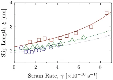
_ is the shear-rate at the bounding surface. The least-squares-fitted linear velocity profile is used to calculate the slip-length (as defined from the CFD surface). Based on the strain-rate/slip-length relationship proposed in [24], and assuming a linear dependence on density, a least-squares fit is per-formed to the following equation:

n¼ðc1ffiffiffiffiffiffiffiffiffiffiffiffiffiffiffiffiffiffi

q

þc2Þ

1

c

_=

c

_c

p ; ð4Þ

where

q

is the density,

c

_cis the critical shear rate (see [24]), and

c1; c2and

c

_ are parameters of the fit to our MD pre-simulations, which are 1:2051012_kg1_m4_{, 3:747}

109_{m and}

200

400

600

1200

1400

1600

Pressure,

p

[MP

a]

Density,

ρ

[kg/m

3

]

(a)

2

3

4

1200

1400

1600

Viscosit

y,

μ

[

×

10

−

4

P

as]

[image:4.595.319.536.72.212.2] [image:4.595.57.263.430.713.2]

Density,

ρ

[kg/m

3

]

(b)

Fig. 2.Data for the Lennard-Jones fluid properties: (a) pressure variation with density, and (b) viscosity variation with density. MD data points from pre-simulation (circles), fitted polynomial (solid lines) and NIST data[26](dashed lines).

0

.

16

0

.

18

0

.

2

1300

1400

1500

1600

1700

Surface

D

isplacemen

t,

δ

[nm]

Density,

ρ

[kg/m

3

]

1:5431011s1_{, respectively.Fig. 4shows our MD pre-simulation} data and the least-squares fit of Eq.(4); data are shown for three different values of density. The slip model approximated by Eqs. (3) and (4)is directly introduced as a Robin boundary condition in the enhanced CFD solver.

2.2. The enhanced CFD model

We use the laminar, compressible flow solversonicLiquidFoam,

which we have modified to (a) accommodate a nonlinear equation of state, (b) allow a density-dependent viscosity, and (c) incorpo-rate slip boundary conditions of the form given in Eq.(4). A com-pressible solver is used despite the very low Mach numbers, since significant compressibility can occur in micro and nano geometries due to very high viscous pressure losses[27,28].

3. Unsteady simulations

We now simulate the unsteady flow behaviour of a Lennard-Jones fluid along a converging–diverging channel; a case chosen to demonstrate the robustness of the enhanced CFD model when applied to non-trivial flow problems.

Owing to the lack of detailed and reliable experimental flow measurements at the nano-scale, in this section we compare our enhanced CFD predictions with full-scale MD simulation results. This comparison is intended to test whether enhanced CFD can produce flow field solutions of comparable accuracy to full MD in complex nano-scale geometries, without the need forad hoc cor-rections, and at only a fraction of the cost of full MD.

3.1. Cases

We consider a two-dimensional geometry: a converging– diverging channel with a smoothly varying height in the stream-wise direction. A gravity-type force is applied to the fluid to gener-ate an unsteady/transient flow. As test cases, we choose flows that exhibit non-continuum behaviour (e.g. slip at surfaces), and do not contain a significant bulk flow region, i.e., the width of the channel is at the 2–3 nm continuum-fluid limit for a Lennard-Jones fluid.

The converging–diverging channel is shown inFig. 5and has a lengthl¼68 nm in the streamwise directionx, a depth of 5.44 nm, and heights of 3.4 nm and 2.04 nm at the inlet and throat sections, respectively. The channel is periodic in both the streamwise and spanwise direction. The height between top and bottom walls

hðxÞvaries in the streamwise direction according to a sinusoidal function,

hðxÞ ¼2a cos 2

p

x l

1

þhinlet; ð5Þ

where 4a¼1:36 nm is the change of height from inlet to throat, and

hinletis the height of the channel at the inlet.

The full MD domain is divided into 200 bins in thex-direction of bin-widthdx¼0:34 nm, and the instantaneous mass flow rate and density are measured in each bin. In the enhanced CFD domain, we define a plane across the channel at equivalent positions, and sum the mass fluxes from each cell the plane crosses, at each time-step, to get the instantaneous data. Dependency studies on the mesh resolution and on the time step showed that 50,000 cells and a time step of 21.6 fs were more than sufficient to obtain converged CFD solutions.

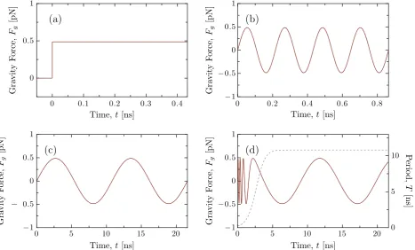
All the flows start from rest, then a time-varying gravity force

FgðtÞis applied. We consider four different forces applied to the fluid:

1. Startup flow: a steady gravity force ofFg¼0:487 pN.

2. Short oscillations: an unsteady, oscillating gravity force with amplitude 0.487 pN and period ofT¼0:22 ns, i.e.

FgðtÞ ¼0:4871012sin

2

p

t 0:22109

; ð6Þ

wheretis the simulation time;

3. Long oscillations: an unsteady oscillating gravity force of the same amplitude, but with a larger periodT¼10:8 ns, i.e.

FgðtÞ ¼0:4871012sin

2

p

t 10:8109

; ð7Þ

wheretis the simulation time;

4. Varying oscillations: an unsteady oscillating gravity force with the same amplitude but with increasing period of 0:2!10:8 ns as shown inFig. 6(d), where the dashed line indicates how the period of the oscillation changes.

2

3

4

0

2

4

6

8

Slip

Length,

ξ

[nm]

[image:5.595.70.268.68.208.2]

Strain Rate, ˙

γ

[

×

10

−10

s

−1

]

Fig. 4.Slip lengthnvarying with strain ratec_for three density valuesq1¼1276 kg/

m3

,q2¼1447 kg/m 3

andq3¼1668 kg/m 3

[image:5.595.87.514.628.742.2]

. MD pre-simulation data points (sym-bols) and fit to Eq.(4)(dashed lines).

[image:6.595.60.528.69.351.2]

Graphical representations of how the forces vary are shown in Fig. 6.

3.2. Results for the four cases

To test the reliability of our CFD predictions that have MD pre-simulation input, we compare results with full-domain molecular dynamics calculations (referred to as ‘full MD’). To test whether our enhanced CFD model is an improvement over conventional CFD, we also compare results with predictions from compressible CFD with no-slip at the wall and without incorporating a CFD sur-face offset (referred to as ‘no-slip CFD’). We also compare with incompressible CFD with slip incorporated but no surface displace-ment (referred to below as ‘incomp. slip CFD’).

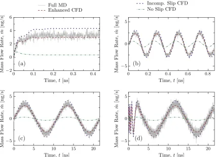
InFig. 7we plot the mass flow rate variation with time in a sin-gle bin near the inlet of the channel for each case. We see that in all cases the enhanced CFD model is able to accurately predict how the mass flow rate changes in time.Fig. 7(a), in which a constant force is applied throughout the channel, shows that the CFD reaches steady state at the same time as the MD simulation, and that a similar final mass flow rate is reached. There are, however, substantial differences between the enhanced CFD, the no-slip CFD, and the incomp. slip CFD results. The oscillations that are observed at the early times inFig. 7(a) in the enhanced CFD results and also the MD data are due to an acoustic response of the nano channel to impulse forcing. A first estimate of the natural acoustic period is obtained byT¼l=c¼0:07 ns (wherec is the speed of sound). This corresponds reasonably closely with the observed kinks in the mass flow rate.

Fig. 7(b) shows the results when an oscillating force with period 0.22 ns is applied. The mass flow rate in the enhanced CFD oscil-lates with the right frequency, the correct amplitude, and is also in phase with the full MD results. The no-slip CFD, on the other hand, appears to have the correct frequency but the amplitude is

incorrect and it is oscillating out of phase, while the incomp. slip CFD is in phase but overpredicts the amplitude.

InFig. 7(c) we have an oscillating force with period 10.8 ns. The mass flux in the enhanced CFD oscillates with the right frequency, correct amplitude, and is in phase, whereas the no-slip CFD appears to have the correct frequency, and is oscillating in phase, but the amplitude is incorrect. InFig. 7(d) the period of the oscil-lating force increases from 0.22 ns to 10.8 ns; even in this more elaborate case, the enhanced CFD prediction is accurate.

Table 1provides an indication of the computational cost for the full-domain MD simulations. The longest simulations presented in this paper ran in parallel (on 24 CPUs) for 48 days. The enhanced CFD itself has negligible computational cost by comparison, although the MD pre-simulations require the computational resources indicated in the last row of Table 1. However, these pre-simulations need only be performed once for a particular fluid/solid combination, and then can be used for any number of flow geometries thereafter.

4. Design optimisation

We now demonstrate how the enhanced CFD model can be used in design optimisation problems at the nanoscale. The example we choose is the optimal design of a bifurcating nano-channel net-work (seeFig. 8); such a design exploration would not be feasible using full MD simulations. The problem is to find the optimal widths of the channels in a bifurcating channel (i.e. those that give greatest mass flow rate), for a constant pressure difference Dp

between the inlet and the outlets, and a constant volumeV. At the macro scale the solution to this problem is given by Murray’s Law[29,30], which was first derived using the Hagen–Poiseuille Law to minimise the power required to sustain the flow of blood through vessels. It has also since been shown to describe the water transport though biological vessels in plants[31], and at the micro

0

0

.

5

1

0

0

.

1

0

.

2

0

.

3

0

.

4

Gra

vit

y

F

orce,

F

g

[pN]

Time,

t

[ns]

(a)

−

1

−

0

.

5

0

0

.

5

1

0

0

.

2

0

.

4

0

.

6

0

.

8

Gra

vit

y

F

orce,

F

g

[pN]

Time,

t

[ns]

(b)

−

1

−

0

.

5

0

0

.

5

1

0

5

10

15

20

Gra

vit

y

F

orce,

F

g

[pN]

Time,

t

[ns]

(c)

−

1

−

0

.

5

0

0

.

5

1

0

5

10

15

20

0

5

10

Gra

vit

y

F

orce,

F

g

[pN]

Time,

t

[ns]

P

erio

d

,

T

[ns]

(d)

scale it has been used to optimally design MEMS devices with rectangular or trapezoidal cross sections[32].

For a 2D two-level network, like the geometry inFig. 8, Murray’s Law is

h20¼

XN

j¼1

h2N; ð8Þ

whereh0is the width of the inlet parent channel, andh1tohNare the widths of the outlet daughter channels. For a symmetric bifur-cating channel withN¼2 andh1¼h2, the optimum ratio of chan-nel widths is then given by

h20

2h21

¼1: ð9Þ

−

2

0

2

4

6

0

0.1

0.2

0.3

0.4

Mass

Flo

w

Rate,

˙

m

[ng/s]

Time,

t

[ns]

Full MD

Enhanced CFD

(a)

₋

5

0

5

0

0.2

0.4

0.6

0.8

Mass

Flo

w

Rate,

˙

m

[ng/s]

Time,

t

[ns]

Incomp. Slip CFD

No Slip CFD

(b)

−

5

0

5

0

5

10

15

20

Mass

Flo

w

Rate,

˙

m

[ng/s]

Time,

t

[ns]

(c)

₋

₅

0

5

0

5

10

15

20

Mass

Flo

w

Rate,

˙

m

[ng/s]

[image:7.595.90.517.67.377.2]

Time,

t

[ns]

(d)

[image:7.595.41.564.453.515.2]

Fig. 7.The mass flow rate near the inlet of the channel varying with time, for each case. The solid lines are the full MD results, the dashed lines are the enhanced CFD results, the dotted lines are the incomp. slip CFD results and the dot dashed lines are the no-slip CFD results. (a) step force, (b) oscillating gravity force with periodT¼0:22 ns, (c) oscillating gravity force with periodT¼10:8 ns, and (d) oscillating gravity force with increasing periodT¼0:22!10:8 ns. Note the statistical noise in the full MD results.

Table 1

Computational costs: the first four rows are for the full MD simulations, while the last row is the MD pre-simulation that is used to collect the data for the enhanced CFD.

CPUs Liquid molecules Wall molecules Time per MD time-step (s) Total computational time

Startup flow 24 69,264 19,677 0.68 16 h

Short oscillations 24 69,264 19,677 0.68 30 h

Long oscillations 24 69,264 19,677 0.68 48 days

Varying oscillations 24 69,264 19,677 0.68 48 days

MD pre-simulations 24 5073–6668 4160 0.14 4 days per liquid/solid combination

[image:7.595.54.532.472.638.2]

The optimisation we perform, with the given constraints of constant volume and fixed pressure difference, is a linear search on channel width (equal increments) to find the maximum mass flow rate. We choose a volume of 1100 nm3_{, a pressure difference of 10 MPa,} channel lengths l0¼l1¼75 nm, a junction lengthlj¼20 nm and junction width,hj¼4 nm. The volumeVcan be calculated as:

V¼h0l0þhjljþ2h1l1: ð10Þ

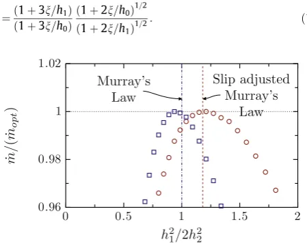
If this geometry was optimised using MD, each simulation would take approximately 30 days, whereas each enhanced CFD sim-ulation takes approximately 500 s to perform. Fig. 9 shows the results from this optimisation with our enhanced CFD model used on a micro-scale channel and on a nano-scale channel. We see that for a micro scale channel, the optimum width occurs when

h2₀=2h2₁¼1: this is the expected result according to Murray’s Law. At the nano-scale, however, we observe a significant deviation from the standard Murray’s Law, which is now discussed.

A deviation from the standard Murray’s Law has been noted for rarefied gases[33]but has not so far been demonstrated for a liq-uid. To uncover the origin of this deviation we derive Murray’s Law using Poiseuille’s equations with Navier slip at the walls, i.e.

uðhÞ ¼uðhÞ ¼ndu

dywherenis the slip length, and the velocity is at a maximum aty¼0 i.e.du

dyjy¼0¼0. The mass flow rate is then

_ m¼2

q

3

l

D

p

l h 3

1þ3n

h

; ð11Þ

wherem_ is the mass flow rate,

q

is the density,

l

is the dynamic vis-cosity andDpis the pressure difference between the inlet of the parent channel and the outlet of the daughter channel. Murray’s Law is found by minimising the powerPrequired to maintain flow, which for flow through a channel is

P¼m_

D

pþ2bhl; ð12Þ

wherebis a constant of proportionality. By eliminatingDpwith Eq. (11) in this equation and differentiating, we find that when the power is minimised the mass flow rate is

_

m¼kh2 ð1þ3n=hÞ

ð1þ2n=hÞ1=2; ð13Þ

where k¼2=3pffiffiffiffiffiffiffiffiffiffiffiffi

q

b=

l

. For a symmetric bifurcating channel, the mass flow rate through the parent channel must equal the total mass flow rate through the daughter channels, i.e.m_0¼2m_1, there-fore, the optimal ratio of channel widths becomes

h20

2h21

¼ð1þ3n=h1Þ ð1þ3n=h0Þ

ð1þ2n=h0Þ 1=2

ð1þ2n=h1Þ

1=2: ð14Þ

It is clear that whenh0;h1nthis becomes Eq.(9), as expected. It can also be noted that when the flow becomes plug-like, i.e.

h0; h1n, this ratio becomesh20=2h 2 1¼2

1=3 .

We can now use Eqs.(10) and (14)to calculate the expected value ofh2₀=2h2₁. When comparing this to the optimum found by the enhanced CFD we get excellent agreement, as highlighted in Fig. 9. This shows that the slip at the walls is the important factor in the deviation from the expected optimum. A CFD model that includes an accurate model of the wall–fluid interaction is, there-fore, potentially very important in the design of nano-scale devices.

5. Summary

We have shown that a CFD model enhanced with data from MD pre-simulations is capable of making accurate predictions of unsteady liquid flow along a converging–diverging channel that has a width close to the expected continuum-fluid limit. This enhanced CFD approach is far more accurate than conventional CFD calculations, and significantly more computationally efficient than full MD simulations.

We have also demonstrated the enhanced CFD approach applied to a design optimisation problem: that of a bifurcating nanofluidic network. The widths of channels in the network should be optimised to maximise the mass flow rate through the network, for a fixed pressure drop and network volume. We have shown that slip at the nano-scale can have a very significant effect on the opti-mum channel dimensions, and we have derived an analytical equa-tion which corrects the well-known Murray’s Law. This is one of many possible cases where nano-scale flow effects modify the optimal design of nanofluidic systems when compared with their macroscopic counterparts.

Acknowledgments

This work is financially supported in the UK by EPSRC Programme Grant EP/I011927/1 and EPSRC Grants EP/K038664/1 and EP/K038621/1. Our calculations were performed on the high performance computer ARCHIE at the University of Strathclyde, funded by EPSRC Grants EP/K000586/1 and EP/K000195/1.

References

[1]Alexiadis A, Kassinos S. Molecular simulation of water in carbon nanotubes. Chem Rev 2008;108(12):5014–34.

[2]Mantzalis D, Asproulis N, Drikakis D. Filtering carbon dioxide through carbon nanotubes. Chem Phys Lett 2011;506(1):81–5.

[3]Saidur R, Leong KY, Mohammad HA. A review on applications and challenges of nanofluids. Renew Sustain Energy Rev 2011;15:1646–68.

[4]Wen D, Lin G, Vafaei S, Zhang K. Review of nanofluids for heat transfer applications. Particuology 2009;7(2):141–50.

[5]Levitt M, Warshel A. Computer simulation of protein folding. Nature 1975;253(5494):694–8.

[6]Parrinello M, Rahman A. Crystal structure and pair potentials: a molecular-dynamics study. Phys Rev Lett 1980;45(14):1196.

[7]Sheehan ME, Sharratt PN. Molecular dynamics methodology for the study of the solvent effects on a concentrated diels-alder reaction and the separation of the post-reaction mixture. Comput Chem Eng 1998;22:S27–33.

[8]Reese JM, Gallis MA, Lockerby DA. New directions in fluid dynamics: non-equilibrium aerodynamic and microsystem flows. Philos Trans Royal Soc Lond Series A: Math, Phys Eng Sci 2003;361(1813):2967–88.

[9]Bocquet L, Charlaix E. Nanofluidics, from bulk to interfaces. Chem Soc Rev 2010;39(3):1073–95.

[10]Huang C, Choi PY, Nandakumar K, Kostiuk LW. Comparative study between continuum and atomistic approaches of liquid flow through a finite length cylindrical nanopore. J Chem Phys 2007;126(22):224702.

[11]Sofos F, Karakasidis T, Liakopoulos A. Transport properties of liquid argon in krypton nanochannels: anisotropy and non-homogeneity introduced by the solid walls. Int J Heat Mass Transf 2009;52(3–4):735–43.

[12]Travis KP, Todd BD, Evans DJ. Departure from Navier–Stokes hydrodynamics in confined liquids. Phys Rev E 1997;55(4):4288.

[13]Todd BD, Hansen JS, Daivis PJ. Nonlocal shear stress for homogeneous fluids. Phys Rev Lett 2008;100(19):195901.

0

0

.

5

1

1

.

5

2

0

.

96

0

.

98

1

1

.

02

h

2

1

/

2

h

22

[image:8.595.47.272.534.714.2]

˙

m/

(˙

m

opt

)

Murray’s

Law

Slip adjusted

Murray’s

Law

[14]Cadusch PJ, Todd BD, Zhang J, Daivis PJ. A non-local hydrodynamic model for the shear viscosity of confined fluids: analysis of a homogeneous kernel. J Phys A: Math Theor 2008;41(3):035501.

[15]Todd BD. Cats, maps and nanoflows: some recent developments in nonequilibrium nanofluidics. Mol Simul 2005;31(6-7):411–28.

[16] Holland DM, Lockerby DA, Borg MK, Nicholls WD, Reese JM. Molecular dynamics pre-simulations for nanoscale computational fluid dynamics. Microfluid Nanofluid.http://dx.doi.org/10.1007/s10404-014-1443-6. [17]Popadic´ A, Walther JH, Koumoutsakos P, Praprotnik M. Continuum

simulations of water flow in carbon nanotube membranes. New J Phys 2014;16(8):082001.

[18]Mohamed KM, Mohamad AA. A review of the development of hybrid atomistic–continuum methods for dense fluids. Microfluid Nanofluid 2010;8(3):283–302.

[19]Borg MK, Lockerby DA, Reese JM. The FADE mass-stat: a technique for inserting or deleting particles in molecular dynamics simulations. J Chem Phys 2014;140(7):074110.

[20]Borg MK, Macpherson GB, Reese JM. Controllers for imposing continuum-to-molecular boundary conditions in arbitrary fluid flow geometries. Mol Simul 2010;36(10):745–57.

[21]Macpherson GB, Borg MK, Reese JM. Generation of initial molecular dynamics configurations in arbitrary geometries and in parallel. Mol Simul 2007;33(15):1199–212.

[22]Macpherson GB, Reese JM. Molecular dynamics in arbitrary geometries: parallel evaluation of pair forces. Mol Simul 2008;34(1):97–115.

[23] OpenFOAM. The open source CFD toolbox; 2015. <http://www.openfoam.org>. [24]Thompson PA, Troian SM. A general boundary condition for liquid flow at solid

surfaces. Nature 1997;389(6649):360–2.

[25]Irving JH, Kirkwood JG. The statistical mechanical theory of transport processes. iv. The equations of hydrodynamics. J Chem Phys 1950;18:817–29. [26] Linstrom PJ, Mallard WG. NIST chemistry webbook. NIST standard reference

database no. 69. <http://webbook.nist.gov>.

[27]Gad-el Hak M. MEMS: introduction and fundamentals. CRC Press; 2010. [28]Patronis A, Lockerby DA, Borg MK, Reese JM. Hybrid continuum–molecular

modelling of multiscale internal gas flows. J Comput Phys 2013;255:558–71. [29]Murray CD. The physiological principle of minimum work: I. The vascular system and the cost of blood volume. Proc Natl Acad Sci USA 1926;12(3):207–14.

[30] Murray CD. The physiological principle of minimum work: II. Oxygen exchange in capillaries. Proc Natl Acad Sci USA 1926;12(5):299–304. [31]McCulloh KA, Sperry JS, Adler FR. Water transport in plants obeys Murray’s

law. Nature 2003;421(6926):939–42.

[32]Emerson DR, Cies´licki K, Gu X, Barber RW. Biomimetic design of microfluidic manifolds based on a generalised Murray’s law. Lab Chip 2006;6(3):447–54. [33]Gosselin L, da Silva AK. Constructal microchannel networks of rarefied gas