Online learning with (multiple) kernels : a review

http://wrap.warwick.ac.uk/

Original citation:

Diethe, Tom and Girolami, Mark, 1963-. (2013) Online learning with (multiple) kernels : a

review. Neural Computation, Volume 25 (Number 3). pp. 567-625. ISSN 0899-7667

Permanent WRAP url:

http://wrap.warwick.ac.uk/64700

Copyright and reuse:

The Warwick Research Archive Portal (WRAP) makes this work by researchers of the

University of Warwick available open access under the following conditions. Copyright ©

and all moral rights to the version of the paper presented here belong to the individual

author(s) and/or other copyright owners. To the extent reasonable and practicable the

material made available in WRAP has been checked for eligibility before being made

available.

Publisher statement:

© 2013 The MIT Press

Link to the journal's homepage:

http://www.mitpressjournals.org/doi/abs/10.1162/NECO_a_00406#.VIcJvTGsV8E

Copies of full items can be used for personal research or study, educational, or

not-for-profit purposes without prior permission or charge. Provided that the authors, title and

full bibliographic details are credited, a hyperlink and/or URL is given for the original

metadata page and the content is not changed in any way.

A note on versions:

The version presented in WRAP is the published version or, version of record, and may

be cited as it appears here.

Online Learning with (Multiple) Kernels: A Review

Tom Diethe [email protected] Mark Girolami [email protected]

Department of Statistical Science, Centre for Computational Statistics and Machine Learning, University College London, WC1E 6BT, U.K.

This review examines kernel methods for online learning, in partic-ular, multiclass classification. We examine margin-based approaches, stemming from Rosenblatt’s original perceptron algorithm, as well as nonparametric probabilistic approaches that are based on the popular gaussian process framework. We also examine approaches to online learning that use combinations of kernels—online multiple kernel learn-ing. We present empirical validation of a wide range of methods on a protein fold recognition data set, where different biological feature types are available, and two object recognition data sets, Caltech101 and Caltech256, where multiple feature spaces are available in terms of dif-ferent image feature extraction methods.

1 Introduction

In its canonical form, the termonline learningrefers to the paradigm where the “learner” (i.e. algorithm) receives data instances and labels in a sequen-tial fashion (Freund & Schapire, 1997). The goal of the learner is to predict the labely_t ∈Y of the instancex_t∈X at timet, after which the true label is revealed. This differs from batch learning, where a (training) data setS

consisting ofmpairs of examples{x_i,y_i}is given, and incremental learn-ing, where multiple batchesS_t,t=1, .. ,Tare given. Typically in batch and incremental learning, it is assumed that the data are generated indepen-dent and iindepen-dentically(iid)from an underlying data-generating distribution D= {X×Y}. In this scenario, the goal of the learner in incremental learn-ing is to build a model that closely approximates the model that would be learned if all the batches of the data were given at once, with computa-tional advantages of efficient incremental updates and processing only on the batch at any one time. Of course, if the size of each batch is 1, this would reduce to the online learning setting, with the assumption that the data are generated i.i.d. However, often online learning algorithms (and the theory associated with them) does not assume that the data are generated i.i.d.

(i.e., the underlying data distribution may be shifting or switching), so this reduction of incremental to online learning is to a restricted case only.

The perceptron algorithm (Rosenblatt, 1958) is an online algorithm that iteratively builds a hyperplane to separate data into two classes. It pro-ceeds by adjusting the hyperplane whenever a mistake is made and has been shown to have favorable convergence properties if the data are lin-early separable (Novikoff, 1962). In the case where the data are noisy, the perceptron may never converge, but this can be alleviated by fixing the model after a period of time or through the use of a regularization term in the cost function. If the goal is to find the hyperplane that best separates the data, it stands to reason that casting this goal as an optimization prob-lem is a sensible thing to do. The support vector machine (SVM) (Vapnik, 1995) does exactly this: it seeks to find the hyperplane that maximizes the margin between two classes of data. It has since been shown that a mi-nor modification of the perceptron (the margin perceptron; see Duda and Hart, 1973) would be equivalent to an unregularized SVM, with the only re-maining difference appearing to be the training method: stochastic gradient descent (SGD) for the perceptron and quadratic programming for the SVM (Collobert & Bengio, 2004). In fact, since the SVM can be solved using SGD as well, this link is probably even deeper (Bordes, Ertekin, Weston, & Bottou, 2005). Since the perceptron has long stood as a benchmark in online learning, it should come as no surprise that the SVM stands as the bench-mark in the batch classification setting, certainly in terms of kernel methods (see section 1.2).

These distinctions will become clearer when we discuss specific algo-rithms, as some algorithms are designed from the batch or incremental perspective, sometimes even requiring that several (pseudo-online) passes over the (batch) data set are required, and others are “true” online. We will refer to the former as “online batch” and the latter as “true online.” This often leads to confusion as often both are referred to as online learning. In fact, it is also possible to distinguish two separate cases in the online-batch setting (approaches based on Monte Carlo sampling techniques): only one pass over the training data, which is known as stochastic approximation (SA), and multiple passes over the training data, which is known as sample average approximation (SAA) (Nemirovski, Juditsky, Lan, & Shapiro, 2009). Neither is related to the true-online setting, but when the data are i.i.d., they can be used to obtain classifiers with generalization error bounds. In SA, the aim is to approximate a problem of the form

min

w R(w)+E[L(w,X,Y)], (1.1)

whereRis the regularization function,wis the solution vector, andLis the loss function. In SAA, the above problem is approximated with

min

w R(w)+

1

T T

i=1

which can be minimized, such as with stochastic methods. The solutions of the algorithms will differ greatly, even if their instantiations are similar (Nemirovski et al., 2009). A full analysis of these methods is outside the scope of this review.

1.1 Online-to-Batch Conversions. Note that in general, it is always

possible to transform an online algorithm into a batch algorithm. From a theoretical perspective, if it is known that the samples are i.i.d., it is possible to transform a regret bound for an online algorithm into a convergence rate or generalization bound for the equivalent batch problem. However the opposite is not true; algorithms that are designed specifically to work with i.i.d. samples with a proven generalization error bound in principle cannot be used in the pure online setting and do not have a regret bound guarantee. Examples of this are the algorthms based on stochastic gradient descent (SGD) analyzed by Zhang (2004). These have finite-sample convergence rate bounds but cannot be used in the online setting without projections (see Zinkevich, 2003).

When an online algorithm is converted to a batch algorithm, the resulting batch algorithm often closely resembles some form of SGD algorithm. This online-to-batch conversion can be carried out in different ways. It may seem like the simplest method is to take the last solution. However, if the algorithm has not yet converged, the last solution may be arbitrarily bad. For convex loss functions, the simplest approach that mitigates this problem is to take the average of all of the solutions generated at each time step, (see Cesa-Bianchi, Conconi, & Gentile, 2004, for details). For nonconvex losses, a complex procedure is also described in Cesa-Bianchi et al. (2004), which enables one to obtain generalization error bounds from regret bounds, such as for the 0–1 loss function of the perceptron algorithm.

We will attempt to disambiguate from a wide set of algorithms that have been proposed, and for a representative selection of these, we evaluate their performance in terms of their true online performance, as well as their online-batch performance, that is, how well the model trained on a data set in an online fashion then performs on a separate test set. We will not consider the incremental setting in this study except where it is necessary for the algorithm to run in a reasonable time frame.

For the purposes of this study, for one set of experiments we use the online-to-batch conversion mechanism described in Cesa-Bianchi et al. (2004)—averaging the hyperplanes generated at each step in the learning phase.

1.2 Kernel Methods in Online Learning. We restrict this survey to

function), as long as the inner productκ(x_i,x_j)= φ(x_i), φ(x_j)can be eval-uated efficiently. In many cases, this inner product or kernel function can be evaluated much more efficiently than the feature vector itself, which can even be infinite-dimensional in principle. For a given kernel function, the associated feature space is not necessarily unique. A commonly used kernel function for which this is the case is the radial basis function (RBF) kernel, defined as

κ_γ(x,z)=exp

−x−z2

γ

. (1.3)

The RBF kernel projects the data into a (nonunique) infinite-dimensional Hilbert space. One drawback, as with most other kernel methods, is that storing large kernel matrices is computationally prohibitive: it requires O(m2_{)data storage.}1_{When kernel methods are used in online learning, this}

data storage requirement is dropped at the expense of extra kernel com-putations. An online algorithm will have to calculate the kernel function between the new data point and any points that are stored from previous rounds that may be used in calculating the decision function or updating of the statistical model at timet. The set of points stored by the algorithm will be called the active set and denoted byAhenceforth. In many cases, it is more practical to store the original data points rather than the kernel evalu-ations, at the expense of the computational cost per iteration. The use of an active set means that the memory requirements at timetare onlyO(|A_t|) (orO(|At|2) if the kernel evaluations are stored) where typically|At| t,

and in many cases can be fixed a priori. We will see that how this active set is created and maintained, together with the statistical model being gener-ated, are the two key features that differentiate between the algorithms we investigate here.

1.3 Online Multiple Kernel Learning. Online learning and kernel

learning are two active research topics in machine learning. Although each has been studied extensively, only recently have efforts in addressing the intersecting research been made. Some early work that did not specifically refer to the multiple kernel learning (MKL) problem examined the situation where a set of “experts” is employed, and relative loss bounds were devel-oped using weighted combinations of these experts (Herbster & Warmuth, 1998).2_{Of course, each expert could be the same algorithm (such as a kernel}

perceptron) using a different feature space, in which case this resembles an MKL approach (and as we will see particularly resembles the approach to

1_{For online learning,m=T. For batch learning,mis then the number of training}

points.

online MKL of Jin, Hoi, & Yang, 2010). However the goal of the framework was to model situations in which the data-generating distribution of the examples changes (or switches), and different experts are best for certain segments of the sequence of examples. The algorithm has been shown to perform well on data organized in temporal blocks (Herbster & Warmuth, 2001; Herbster, 2001). Here we restrict ourselves to algorithms that attempt to find a stable combination of the feature spaces. Two notable approaches to online multiple kernel learning (OMKL) have been made, both of which try to learn a kernel-based prediction function from a pool of predefined kernels (or kernel functions) in the online learning framework (Jin et al., 2010; Luo, Orabona, Fornoni, Caputo, & Cesa-Bianchi, 2010). The problem of OMKL is generally more challenging than typical online learning be-cause both the kernel classifiers and the (linear) combination of these must be learned simultaneously. The specific approaches outlined by Jin et al. (2010) and Luo et al. (2010) are discussed in section 3.3.

1.4 Probabilistic Online Learning. Another approach to the online

learning problem is the probabilistic or Bayesian approach. Traditional Bayesian inference requires the definition of prior and likelihood distri-butions, and then computation of the posterior conditioned on the data and the prior. In the online setting, the true posterior distribution is re-placed with a simpler parametric distribution, and following on from this, one can define an online algorithm by alternating between updates of the approximate posterior when a new example arrives, and an optimal projection into the parametric family (Opper, 1998). Predictions are made by averaging over the approximate posterior. It was also suggested that minimizing the difference between the batch and the approximate poste-rior optimizes the performance of the Bayes online algorithm (Winther & Solla, 1998). These methods were demonstrated in neural network learning (Opper, 1998) and linear perceptron learning with binary or continuous weight priors (Winther & Solla, 1998).

vectors also being chosen online (again forming an active set again). There have been several attempts to do this, notably sparse online gaussian pro-cesses (SOGP) (Csat ´o & Opper, 2002), the virtual vector machine (VVM) (Minka, Xiang, & Qi, 2009), and predictive active set selection methods for gaussian Processes (PASS-GP) (Henao & Winther, 2010). These methods are discussed further in section 3.5.

1.5 Outline. The rest of the review is set out as follows. In section 2, we formally introduce the notation that will be used throughout the review. In section 3, we describe each of the algorithms that we will be examin-ing. These will be presented in (roughly) chronological order and divided into several subsections: those that come from a decision-theoretic perspec-tive (section 3.1), perceptron based (section 3.2), margin-based perspecperspec-tive (section 3.2.4), and those that come from a probabilistic (Bayesian) perspec-tive (section 3.5). In section 4 we provide extensive empirical testing of the proposed methods, and in section 5 we conclude with a discussion.

2 Preliminaries

In the binary online classification framework with a single feature space, we assume that at timet, we are given an examplex_t ∈Rn, and the goal is to make a predictionyˆ_t ∈ {−1,1}, after which the true labely_t∈ {−1,1}is revealed.

DefineI(z)as the indicator function that returns 1 ifz>0 and 0 other-wise, sgn(z)as the function that returns−1 ifz<0 and 1 otherwise,1as a vector of all ones,I∈Rm×m_{as them-dimensional identity matrix, andz}

I

as the vector indexed by the index setI.zandAdenote the transposes of the vectorzand matrixA, respectively.

We aim to learn a linear function f(x)= w, φ(x), which due to the rep-resenter theorem can be rewritten in the form f(x)=_iα_iφ(x_i), φ(x) =

iαiκ(xi,x), where κ is the kernel function described in the following

definition:

Definition 1. A kernel is a functionκthat for allx,z∈Xsatisfies

κ(x,z) =φ(x), φ(z),

whereφis a mapping fromXto an (inner product) Hilbert spaceH,

φ:X →H.

In the multiple kernel learning setting, we are given a finite number of kernel functions (a kernel family)κ_β= {κ₁, . . . , κ_k}, which can be combined using a convex combination as follows:3

κ_β(x,z)= k

j=1

βjκj(x,z), withβj≥0,

k

j=1

βj=1, (2.1)

wherex,z∈Rn_.

The explicit feature mapping induced by each kernel function is defined

asφ_j:x→φ_j(x)∈H_j,j=1, . . . ,k, whereH_jis the Hilbert space of thejth

feature space. We will denote the set of weight vectors for each feature map

asw¯ = {w₁, . . . ,w_k}and the kernel coefficients asβ=(β₁, . . . , β_k).

2.1 Batch Multiple Kernel Learning. The primal optimization of

mul-tiple kernel learning (MKL) (which we refer to as “₁MKL”), as defined in Rakotomamonjy, Bach, Canu, and Grandvalet (2008), can be written as

min 1 2

k

j=1

1

βj

w_j2

+C

m

i=1 ξi

w.r.t. w¯ ∈Rn×k_,β∈Rk_,ξ∈Rm_,b∈R,

s.t. y_i

_k

j=1

w_j, φ_j(x_i) +b

≥1−ξ_i, i=1, . . . ,m,

ξ_i≥0, i=1, . . . ,m,

k

j=1

βj=1, βj≥0, j=1, . . . ,k, (2.2)

with the following decision rule,

f(x)=sgn

_k

j=1 β∗

jw∗jφj(x) +b∗

=sgn _k

j=1 β∗

j m

i=1 α∗

iκj(x,xi)+b∗

=sgn _m

i=1 α∗

iκβ(x,xi)+b∗

, (2.3)

3_{There exist other combinations such as linear combinations (as convex but without}

whereκ_β is defined as in equation 2.1. The₁norm penalty on the kernel coefficients leads to a sparse subselection of kernels in the kernel combina-tion. This is often seen as desirable for computational and interpretability reasons, but a sparse subselection of kernels may not always be desirable. The formulation above can be generalized to the case of generic_pnorms,

p≥1 (see, for example, Kloft, Brefeld, Sonnenburg, & Zien, 2011). It will also be useful to define the_2,p-group norm ¯w_2,pofw¯ as

¯w_2,p= . (w₁₂,w₂₂, . . . ,w_k2)_p

2.2 Gaussian Processes for (Online) Classification. Here we briefly

review the application of gaussian processes for classification and how they are used in an online setting.

A gaussian process is defined as a gaussian distribution over latent func-tions. Given the consistency property of gaussian distributions, whereby marginals are also gaussian, pointwise evaluations at the data points

f=[f(x₁), . . . ,f(x_T)]T _{are jointly gaussian. By specifying a covariance}

functionC(x,x)and a mean functionh(x), we see thatf∼N(h,K)where

h=[h(x₁, . . . ,x_T)] andKis the covariance matrix, which is equivalent to the

Gram matrix in kernel methods. Since the data points appear in the expres-sion only through the covariance matrix, and hence through inner products, any nonlinear mapping that produces valid covariances (kernels) can be used, as before. For classification, it is assumed that the labels are observed independently, and a probit likelihood functiong(y_t|f(x_t))=Q(f_ty_t)where

Q(·)is the gaussian cumulative density function.4_{The (intractable)}

poste-rior is then

p(f|X,y)= 1

Zp(f|X)

T

t=1

g(y_t|f(x_t)),

where the normalizing constantZ=p(y|X)is the marginal likelihood. Cur-rently the most accurate deterministic approximation to this is through the use of expectation propagation (EP) (Rasmussen & Williams, 2005). In EP, the likelihood is approximated by an unnormalized gaussian to give

p(f|X,y)= 1

Z_EPp(f|X)

T

t=1

1

Z_tg˜(yt|f(xt)),

= 1

Z_EPp(f|X)N(f| ˜h,C˜),

=N(f|h,C),

whereZ_EPandZ_tare normalization coefficients,g(y_t|˜f(x_t))andN(f| ˜h,C˜)

are the gaussian approximations tog(y_t|f(x_t))at each sitex_t. In order to obtain the full (approximate) posteriorq(f|X,y), one would start by using the prior,q(f|X,y)=p(f|X), and update each site approximationg˜(·) se-quentially. In order to do this, the so-called cavity distributionq˜(f|X,y_t)

is used—the current posterior with the pointx_t removed. In the “online” methods of Csat ´o and Opper (2002), Lawrence et al. (2002), and Henao and Winther (2010), the full posterior approximation is achieved only after (at least one) full pass through the data set. If time is unbounded, then this method is not possible. The alternative is to process the data in minibatches, where the EP step is run each time a batch of points is included, with the predictions of those points being made on the basis of the model at the previous time step. Of course, if the batch size is set to 1, this would be a true online setting, but the EP updates are generally too expensive to com-pute at that frequency. There is a further problem: unless some kind of active set is used, all of the data points up to timetwould be required, which would lead to an unbounded increase in computational complexity. Csat ´o and Opper (2002), Lawrence et al. (2002), and Henao and Winther (2010) all use an “active set”; they store a restricted set of data points used for EP updates. The methods are differentiated by how examples are in-cluded and exin-cluded from the active set, which we discuss in section 3.5. Another approach, known as the virtual vector machine Minka et al. (2009), which we also discuss, is to use “virtual vectors”—vectors that are created by merging existing data points—as a proxy for the full data set.

2.3 Multiclass Classification. Most linear classifiers, whether online or offline, can be naturally generalized to multiclass classification. Here, the inputxand the outputyare drawn from the label setY. The classification function (or latent function in the GP setting) f(x,y)maps each possible input-output pair to a finite-dimensional real-valued feature vector. The resulting score is used to choose among many possible outputs:

ˆ

y_t =arg max

y∈Y

f(x_t,y).

For example, in the case of the perceptron algorithm, the functionfwould simply be f(x_t,y=y_j)=w_jx_j. The notion of the kernel-defined feature space can be extended to be defined jointly on the spaceX×Y, in which case f(x_t,y=y_j)=w_jφ_j(x_j,y_j)(see Fink & Singer, 2006). In the multiclass setup, with multiple feature spaces, for each classy_j,j=1, . . . ,C, we define

φj(xj,yj)=(0, . . . ,0, ψj(xj)

y_j

whereψ_j(·)is a label-independent feature map. Similarly,wconsists ofC

blocks, and hence by constructionwφ_j(x_j,y_j)=w_jψ_j(x_j).

3 Online Learning with Kernels

In this section, we describe a range of the different approaches to online learning that have been proposed, with particular attention to those that have been extended using kernel methods.

3.1 Decision-Theoretic Approaches. The Hedge algorithm (Freund &

Schapire, 1997; Vovk, 1998) is an algorithm for prediction with expert advice, which comes from a decision-theoretic generalization of online learning. Freund and Schapire (1997, theorem 2) prove that for any sequence of outcomes,

L_T≤ ln 1/β

1−βLT(k)+ lnK

1−β,

for allTandk, whereβ∈[0,1] is a parameter,L_Tis the loss suffered by the algorithm over the firstTtrials andL_T(k)=T_t=1ωt

kis the loss (or expected

loss) suffered by thekth expert over the firstTtrials. The inequality above was improved by Vovk (1998) using the strong aggregating algorithm,

L_T≤c(β)L_T(k)+ c(β)

ln(1/β)lnK,

wherec(β)=(ln1_β)/(Kln_K+K_β−1). The same method can be applied if the experts and the algorithm provide the probability distribution over the outcome space and they suffer the expected loss of a decision randomly selected according to this distribution. In this case, the algorithm predicts simply the weighted average of the experts predictions. The theoretical bound for the loss of the Hedge algorithm is

L_T≤L_T(k)+√2LlnK+lnK.

The constantLis a prior upper bound on the loss of the best strategy and in the worst case isTL, whereLis the bound for the loss used. The weights are updated by the rulew_k:=w_kβλk, whereβ= 1

1+√2 lnK/L, and then they are

Jin et al. (2010) which uses the Hedge algorithm to combine multiple kernel perceptrons.

Under a framework of the “best expert” (Herbster & Warmuth, 1998), worst-case loss bounds for online algorithms were generalized to the case where the additional loss of the algorithm on the whole sequence of exam-ples was bounded over the loss of the best expert (which cannot be known a priori). The sequence is partitioned into segments, and the goal is to bound the additional loss of the algorithm over the sum of the losses of the best experts of each segment. The idea behind this was to model situations in which the examples change and different experts are best for certain seg-ments of the sequence of examples, which may happen if the underlying probability distribution is multimodal or there are switches between phases in the data (e.g., caused by underlying trends or transient states). In the sin-gle expert case, the additional loss is proportional to log(k), wherekis the number of experts and the constant of proportionality depends on the loss function. When the number of segments is at mosts+1 and the sequence of length, the additional loss of their algorithm can be bounded over the best partitioning byO(slog(k)+slog(/s)). The algorithms for tracking the best expert are simple adaptations of Vovk’s original algorithm for the single best expert case. These algorithms keep one weight per expert and spendO(1)time per weight in each trial. The results were later extended to linear combinations (Herbster & Warmuth, 2001).

3.2 Perceptron and Variants. The perceptron was proposed as a

bio-logically plausible model for learning from vectorial data, where a learning rule is constructed that is a linear combination of the examples (Rosenblatt, 1958; Block, 1962; Vapnik & Chervonenkis, 1964). Novikoff (1962) showed that the perceptron algorithm converges after a finite number of iterations if the data set is linearly separable. The idea of the proof is that the weight vector is always adjusted by a bounded amount in a direction that it has a negative dot product with, and thus can be bounded above by,O(√δ), whereδis the number of changes to the weight vector. Furthermore, it can also be bounded below byO(δ)because if there exists an (unknown) satis-factory weight vector, then every change makes progress in this (unknown) direction by a positive amount that depends on only the input vector. This can be used to show that the numberδ of updates to the weight vector is bounded by R_γ22, whereRis the radius of the2-norm ball enclosing the

input space andγ is the margin (the distance between the closest points from each class).

Note that the decision boundary of a perceptron is invariant with respect to scaling of the weight vector that is, a perceptron trained with initial weight vectorwand learning rateτ, results in an identical classifier to a perceptron trained with initial weight vector w

τ, and learning rate 1. Thus,

iterations, the learning rate does not matter in the case of the perceptron and is usually just set to one.

3.2.1 Kernel Perceptron. The perceptron algorithm was first extended

for use in kernel-defined Hilbert spaces by Freund and Schapire (1999), resulting in the kernel perceptron (KP). In addition they combined the classical perceptron algorithm with Helmbold and Warmuth’s (1995) leave-one-out method in order to perform the online-to-batch conversion.5 _The

resulting algorithm is simpler to implement and much more efficient in terms of computation time than the SVM, while the performance is close to (but not as good as) the performance of maximal-margin classifiers on the same problem.

3.2.2 Budgeted Perceptron Variants. If the data are not linearly separable,

the (kernel) perceptron algorithm will never stop updating, meaning that the size of the support set is unbounded. For most practical problems, this makes it impractical for most real-world problems. The first approach to bound the growth of the support set was the budget perceptron (Crammer, Kandola, & Singer, 2003), which removes seemingly redundant examples from the support set by examining the margin conditions of old examples. This was later improved (tigher budget perceptron) by Weston, Bordes, and Bottou (2005) to account for noisy data sets. However, neither of these algorithms has any performance guarantees in terms of bounded numbers of errors. The forgetron (Dekel, Shwartz, & Singer, 2008) was the first budget perceptron that had a formal performance guarantee. It enforces a strict bound on the size of the active set by removing vectors. First, the weights of every vector in the active set are reduced; then it discards the oldest vector in the active set, which has the smallest weight. This is done only when the size of the active set exceeds the budget, so applying this removal procedure on every error will ensure that the size of the active set will not exceed the budget. Due to the repeated weight reductions, the oldest vector will have small weight, so removing it will not change the decision function significantly. The factor by which the forgetron reduces weight is not constant and differs from error to error.

The randomized budget perceptron (RBP) of Cavallanti, Bianchi, and Gentile (2007) is considerably simpler than the forgetron: whenever it makes an error and the size of the active set exceeds the budget, a vector is chosen at random from its active set to be discarded. It was shown that both of these algorithms have bounds of similar order (Sutskever, 2009). Another algorithm, the projectron (Orabona, Keshet, & Caputo, 2009), has been pro-posed in which the instances are not discarded but projected onto the space spanned by the previous online hypothesis. The authors derive a relative

mistake bound and compare the algorithm both analytically and empiri-cally to the forgetron, showing favorable results. Since the RBP is by far the simplest of the budgeted perceptron algorithms, we used this method in the experiments. We also ran preliminary experiments with the projectron, but when compared to the RBP, we found it to be much slower without discernable performance gains.

3.2.3 Relation Between the Perceptron and the Support Vector Machine. For

linearly separable data, the perceptron algorithm can be modified such that it seeks to find the largest separating margin between the classes. The “perceptron of optimal stability” can be solved through iterative schemes, such as the AdaTron (Anlauf & Biehl, 1989), which exploits the fact that the corresponding quadratic optimization problem is convex. The perceptron of optimal stability is, together with the kernel trick, one of the conceptual foundations of the SVM. Later it was shown that the SVM solution could be approximated by the kernel Adatron with an exponentially fast rate of convergence to the optimal solution (Friess, Cristianini, & Campbell, 1998), which completes the link. Note, however, that the Adatron falls under the category of online-batch algorithms rather than being a true online algorithm.

3.2.4 Online Support Vector Machines. Following on from the AdaTron

algorithm, several attempts have been made to adapt the SVM for online learning. The incremental and decremental SVM (Cauwenberghs & Poggio, 2000) is an online recursive algorithm for training SVMs using “adiabatic increments.”6_{An adiabatic process in thermodynamics is one in which heat}

transfer is zero. Here it refers to the “equilibrium” of the training data—that KKT conditions are satisfied for the whole data set, which, in a number of analytical steps, ensure that the KKT conditions (Kuhn & Tucker, 1951) are satisfied on all previously seen training data. Interestingly, the incremental procedure is reversible, and decremental “unlearning” offers an efficient method to exactly evaluate leave-one-out generalization performance, as well as giving some intuition about the relationship between generalization and the geometry of the data. However, since the algorithm requires the storage of the inverse of the Jacobian (second derivatives of the objective function), which scales as|A|2_{, which is in turn unbounded, the algorithm}

is more suited as an online-batch approach than a true online algorithm. Kivinen, Smola, and Williamson (2002) combine classical stochastic gra-dient descent within a feature space and some straightforward tricks to develop simple and computationally efficient algorithms for a wide range

6_{An adiabatic process in thermodynamics is one in which heat transfer is zero. Here it}

of problems such as classification, regression, and novelty detection. The authors specifically consider using online large margin classification algo-rithms in a setting where the target classifier may change over time, but they also show how to exploit the kernel trick in an online setting. They show that their naive online regularized-risk minimization algorithm (NORMA) has appealing worst-case loss bounds and converges to the minimizer of the regularized risk functional. A similar approach was taken to create the implicit online learning with kernels (ILK) and sparse ILK (SILK) al-gorithms (Cheng, Vishwanathan, Schuurmans, Wang, & Caelli, 2006). An implicit update technique was used that can be applied to a wide variety of convex loss functions. The authors prove loss bounds, analyze the con-vergence rate of both algorithms, and show that empirically the algorithms outpeform NORMA.

Later, a family of margin-based online learning algorithms was devel-oped for various prediction tasks under the umbrella term of online SVM and passive agressive (Crammer, Dekel, Keshet, Shalev-Shwartz, & Singer, 2006). The update steps of the algorithms are based on analytical solutions to simple constrained optimization problems. This allowed them to prove worst-case loss bounds for the different algorithms and for the various de-cision problems based on a single lemma. The bounds on the cumulative loss of the algorithms are relative to the smallest loss that can be attained by any fixed hypothesis, as in the “best expert” framwork (Herbster & War-muth, 1998), and as such are applicable to both realizable and unrealizable settings.

Bordes et al. (2005) present another online variant of the SVM, LASVM, an approximate SVM solver that uses online approximation and was shown empirically to reach accuracies similar to that of a real SVM after performing a single sequential pass through the training examples. The authors also show that additional benefits can be achieved using selective sampling techniques to choose which example should be considered next—so-called active learning, which was introduced in the context of the SVM by Tong, Koller, and Kaelbling (2001). The algorithm alternates between two steps: process, which decides whether a point should be added into the active set, and reprocess, which examines the active set to see if any points should be removed. For each data vector, these steps can be repeated several times. The algorithm is fast and performs well in the online-batch setting, but this time suffers from the need to choose both theCparameter (SVM regularization parameter) and an additionalτparameter (for active set inclusion) a priori, which limits its use in a true online setting.

onto the set obtained so far, dramatically reducing time and space require-ments at the price of a negligible loss in accuracy. This is similar in flavor to the projectron algorithm (Orabona, Keshet, & Caputo, 2009).

3.3 Online Multiple Kernel Learning. Recently there have been

at-tempts to extend the multiple kernel learning (MKL) (Bach, Lanckriet, & Jordan, 2004; Lanckriet, Cristianini, Bartlett, Ghaoui, & Jordan, 2004; Rako-tomamonjy et al., 2008) framework to the online learning setting. An incre-mental multiple kernel learning (IMKL) approach was proposed for object recognition that initializes on a generic training database and then tunes itself to the classification task at hand (Kembhavi, Siddiquie, Miezianko, McCloskey, & Davis, 2009). Their system simultaneously updates the train-ing data set as well as the weights used to combine multiple information sources. An online approach to MKL for structured prediction was outlined (Martins, Smith, Xing, Aguiar, & Figueiredo, 2010) using a new family of online proximal algorithms. These algorithms can be used for MKL as well as for group-lasso (Bach, 2008) and variants thereof, and the authors give regret, convergence, and generalization bounds for the proposed methods. However, in the empirical evaluations, they state that multiple passes are required, meaning that the algorithms are not well suited to the true online setting.

3.3.1 OM2 Algorithm. Luo et al. (2010) introduced a theoretically

moti-vated and efficient online learning algorithm for the multiclass MKL prob-lem called OM2. For this algorithm, they prove a theoretical bound on the number of multiclass mistakes made on any arbitrary data sequence. More-over, they show empirically that its performance is on par with, or better than, standard batch MKL, such as SimpleMKL (Rakotomamonjy et al., 2008) algorithms.

Using the group norm notation described above, the MKL problem can be defined in generic form as

min ¯

w

λ

2 ¯w

2

2,1+

T

t=1

Lw¯,x_t,y_t,

which can be extended to the more general_2,pcase as

min ¯

w

λ

2 ¯w

2

2,p+

T

t=1

Lw¯,x_t,y_t,

Shalev-Shwartz, & Tewari, 2009), in which the loss function is replace by its subgradient, meaning that at each step, the following optimization problem must be solved,

¯

w_t=arg min ¯

w

ηw¯

t−1

i=1

∂L(w¯_i,x_i,y_i)+R(w¯),

whereR(·)is a regularization function andη >0 is a parameter. The lin-earization of the loss function through the subgradient provides an efficient closed form for the updates and allows regret bounds to be proven. The so-lution of the above gives the following update,

¯

w_t= ∇R∗

−η

t−1

i=1

∂Lw¯_i,x_i,y_i

,

whereR∗ _{is the Fenchel conjugate ofR, defined asR}∗_(u)=sup

v∈S(vu−

R(v)). For the OM2 algorithm using the_2,p-norm formulation, the regu-larizer isR(w¯)= ₂q ¯w2_2,p, and therefore

R∗_(θ¯)= 1 2q¯θ

2

2,q,

∇R∗_(θ¯)=1

q

θ_j2 ¯θ2

2,q

q−2

θj, j=1, . . . ,k,

which is then used to make updates whenever a mistake is made or when the multiclass loss is greater than 0. The authors further propose a variant of the “follow the regularized leader” framework in which the parameter

η=ηtis changed at each time step if a mistake is made (see algorithm 1 in

Luo et al., 2010) and prove that the cumulative number of mistakes made on any sequence ofTobservations is roughly equal to the optimum value of the original MKL problem.

3.3.2 OMKL Algorithm. Recently an approach to online multiple kernel

sampling strategies. The methods are derived from a single simple exten-sion of the kernel perceptron (KP); the idea is to combine the outputs from KPs learned on each feature space separately using the Hedge algorithm. In effect, this makes it more of a classifier combination algorithm than a true MKL algorithm, but we will continue to call the algorithm OMKL in the rest of this review. Mistake bounds are derived for all the proposed OMKL algorithms, along with pseudo-code for the algorithms, but no experimen-tal results are given, and in fact no implementation has been tested before now.7

We chose to focus on the first two algorithms, DA for OMKL-P (1) and DA for OMKL-P (2), the only difference between the two being that the second version allows for misclassifications (at the cost of an extra parameter), whereas the first one does not. However in practice, we found very little difference in performance between the two and therefore chose to use the first variant because it has only one parameter (the discount parameterβ).

3.4 Boosting and Random Forest Approaches to Online Learning.

Re-cently a set of methods has been proposed that extend the boosting (Freund & Schapire, 1997) and random forest (Breiman, 2001; Bosch, Zisserman, & Munoz, 2007a) methods to the online setting; it is called online multi-class LPBoost, online multimulti-class gradient boost, and online random forest (Saffari, Leistner, Santner, Godec, & Bischof, 2009; Saffari, Godec, Pock, Leistner, & Bischof, 2010). These were designed for object detection in im-ages. These are not kernel methods per se, as the nonlinearity comes through the use of so-called weak learners. However the link between ₁-norm MKL and LPBoost has been observed (Hussain & Shawe-Taylor, 2010). This perhaps provides a further avenue for research for the derivation of new multiclass MKL methods.

3.5 Probalistic Approaches to Online Learning. The first attempt to

discuss online learning from the viewpoint of Bayesian statistical inference was that of Opper (1998) and Opper and Winther (1999). By replacing the true posterior distribution with a simpler parametric distribution, one can define an online algorithm by a repetition of two steps: an update of the approximate posterior, when a new example arrives, and an optimal projection into the parametric family. Choosing this family to be gaussian, Opper showed that the algorithm achieves asymptotic effciency.

The most interesting approaches to online learning in a probabilistic set-ting have been online and incremental approaches gaussian proscess (GP) regression and classification. One of the first attempts to create an online ap-proximation of the GP model was the sparse online GP of Csat ´o and Opper (2002). The authors developed an approach for sparse representations of GP

models in order to overcome their limitations caused by large data sets. The method is based on a combination of a Bayesian online algorithm together with a sequential construction of an active set that fully specifies the predic-tion of the GP model. By using an appealing parametrizapredic-tion and projecpredic-tion techniques that use the RKHS norm, recursions for the effective parameters and a sparse gaussian approximation of the posterior process are obtained. This allows both a propagation of predictions and Bayesian error measures. However, the repeated projections into low-dimensional subspaces can be computationally costly because they require matrix multiplications.

Around the same time, the informative vector machine (IVM) was pro-posed as a practical method for gaussian process regression and classifica-tion (Lawrence et al., 2002). The IVM produces a sparse approximaclassifica-tion to a gaussian process by combining assumed density filtering (Opper, 1998) with a heuristic for choosing points based on minimizing posterior entropy. This is notionally simper than the approach of Csat ´o and Opper (2002), while obtaining similar results.

A method for the sparse greedy approximation of GP regression was given by Seeger, Seeger, Williams, Lawrence, and Dp (2003), featuring a novel heuristic for very fast-forward selection. The advantage of this method is that it is essentially as fast as an equivalent one that selects the support patterns at random yet was shown to outperform random selec-tion on difficult curve-fitting tasks. More important, it leads to a sufficiently stable approximation of the log marginal likelihood of the training data, which can be optimized to adjust a large number of hyperparameters auto-matically. It is, however, limited to the regression setting.

Minka et al. (2009) took a slightly different approach, the virtual vec-tor machine (VVM), in which information contained in the preceding data stream is summarized by a gaussian distribution of the classification weights plus a constant number of “virtual” data points, which are de-signed to include nongaussian information about the classification weights and in theory allows a smooth trade-off between prediction accuracy and memory size. To maintain the constant number of virtual points, the vir-tual vector machine adds the current real data point into the virvir-tual point set, merges the two most similar virtual points into a new virtual point, or deletes a virtual point that is far from the decision boundary. The infor-mation lost in this process is absorbed into the gaussian distribution. The authors suggest that the extra information provided by the virtual points leads to improved predictive accuracy over previous online classification algorithms.

inactive points, allowing points to be removed again from the active set. This is important for keeping the complexity down and at the same time focusing on points close to the decision boundary. The authors demonstrate state-of-the-art results (e.g., 0.86% error on MNIST) with reasonable time complexity.

One approach that has tried to bridge the gap between probabilistic- and optimization-based methods for online learning is TONGA (topmoumoute online natural gradient algorithm; Roux, Manzagol, & Bengio, 2007). The approach is guided by the goal of obtaining an optimization method that is both fast and yields good generalization, and to this end they study the descent direction that maximally decreases the generalization error or the probability of not increasing generalization error. From both Bayesian and frequentist perspectives, this can yield the natural gradient direction; although this can be expensive to compute, an efficient, general, online ap-proximation is possible. This may be a possible avenue forward for unifiying the two approaches.

Another general approach to the problem of extracting informative ex-emples from a data stream is stream greedy (Gomes & Krause, 2010). The authors state that this method includes diverse approaches such as exemplar-based clustering and nonparametric inference, such as GP regres-sion, on massive data sets. They show that the common theme underlying these problems is the maximization of a submodular function that captures the informativeness of a set of examples over a data stream. The stream greedy algorithm is guaranteed to obtain a constant fraction of the value achieved by the optimal solution to these NP-hard optimization problems, and could therefore provide a way of improving the efficiency of proba-bilistic methods such as PASS-GP.

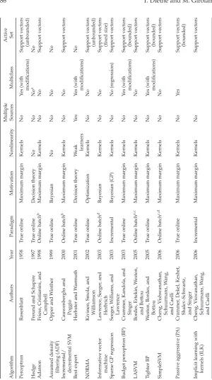
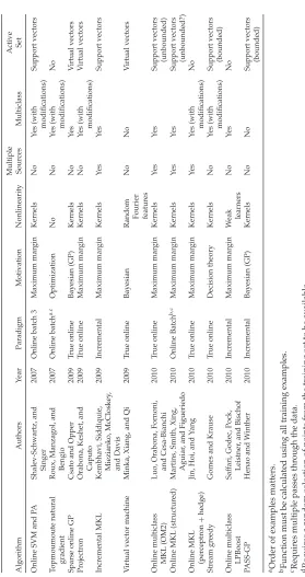
Table 1 gives a taxonomy of the methods discussed in (roughly) chrono-logical order.

3.6 Selection of Kernel Hyperparameters in Online Learning. If linear

kernels are being used, the kernel functionκ is simply the inner product between data examples, so there is no problem using this form of kernel in online learning. However, when nonlinear mappings are used, such as those defined by the RBF kernel functionκ_γas defined in equation 1.3, usually one or more hyperparameters need to be chosen. In the batch learning setting, a heuristic method such asκ-fold cross-validation is performed on the training set, and then the best parameter over thek-folds is used to retrain the model before testing on a separate test set. With no such deliniation between training and testing phases, the choice of kernel hyperparameters is clearly a tricky problem in the online learning setting. Among the several possible approaches to this problem are these:

r

be run using a range of parameters, and the model chosen would be the one with the highest cumulative accuracy aftermsteps. The problem with this method is that without knowing which model will be selected, the predictions for the firstmpoints will have to be made by randomly choosing a classifier from the pool of classifiers, arbritarily selecting one of them, using a voting scheme, or some other classifier combination method.

r

range of kernel functions for each feature space and each parameter setting. The algorithm would then select from among these automat-ically to find the best hyperparameters. This would lead to a large number of possibly redundant kernels and, consequently, a large number of unnecessary kernel evaluations.

r

more recent Bernstein races (Heidrich-Meisner & Igel, 2009) are a technique for finding a good model from a selection of models by quickly discsarding bad models and concentrating the computational resources on differentiating among the better ones. These methods provide a more principled approach than the pseudo-validation set and offer a promising avenue of research.

r

learning (RL) develops replacing-kernel RL (RKRL) (Reisinger et al., 2008), an online model selection method for gaussian process tempo-ral difference (GPTD: a Bayesian RL model by Engel, Engel, Mannor, & Meir, 2005) using sequential Monte Carlo (SMC) methods Doucet, De Freitas, & Gordon, 2001). SMC is used to select good kernel hy-perparameter settings by choosing models according to their relative predictive likelihood instead of the true model likelihood. As a result, RKRL devotes more time to evaluating hyperparameter settings that correspond to areas with high predictive likelihood (i.e., maximizes online reward). When GPTD is used, the current value function esti-mate is formed from the combination of the kernel parameterization determining the prior covariance function and the dictionary gath-ered incrementally from observing state transitions. Each sampling step increases information about the predictive likelihood in the sam-ple (exploitation), while sampling from the transition kernel reduces such information (exploration). This approach is certainly promising for the gaussian process–based approaches.

r

introduced (Zhuang, Tsang, & Hoi, 2009). It would be interesting to investigate possible online extensions of this methodology.

The application of these methods is outside of the scope of this study but offers several potential avenues for further research.

3.7 Normalization. Normalizing features (so that each feature has₂ -norm one across all training examples) or standardizing them (so that each feature has mean 0 and standard deviation 1 across all training examples) is known to be important for regularized linear classifiers or kernel classifiers (Duda & Hart, 1973; Shawe-Taylor & Cristianini, 2004). Empirically this has been shown to be especially important for MKL (Bach et al., 2004; Lanckriet et al., 2004), whether the kernels are linear or nonlinear. Kloft et al. (2011) suggest that the importance of normalization is owed to the bias introduced by regularization. As the optimal feature and kernel weights are requested to be small by imposing penalties on their norms, it stands to reason that this will be easier to achieve for features (or entire feature spaces, as implied by kernels) that are scaled to be of large magnitude, while downscaling them would require a correspondingly upscaled weight for representing the same predictive model. Hence the upscaling or downscaling of features is equivalent to modifying regularizers such that they penalize those features less or more. Generally the solution to this is to use isotropic regularizers, which penalize all dimensions uniformly. As a result, the kernels should be normalized (or standardized) in a sensible way in order to represent an isotropic prior over the features and the feature spaces, one that penalizes all weights in the same way.

Kloft et al. (2011) describe several approaches to normalization and use two particular types in their empirical analysis. They describe these methods:

1. Multiplicative normalization. As described by Shawe-Taylor and

Cristianini (2004) and examined empirically by Zien and Ong (2007), this involves normalizing the kernels to have uniform variance of data points in the features space. Normally this method is combined with centering (the empirical mean of the data points in the feature space lies on the origin), which simplifies the normalization rule.

2. Spherical normalization.Each data point is rescaled to lie on the

unit sphere. This may also have an effect on the scale of the fea-tures, as a spherically normalized and centered kernel is also always multiplicatively normalized.

3. Input space normalization. Each data point is normalized in the

original space.

5. Incremental standardization.The mean and standard deviation of each feature within each feature space are updated incrementally using the update equations (see equation 3.1). Note, however, that the active set needs to be restandardized at each step as well,8_leading

to additional computational burden not found in methods 3 and 4:

μt=

t−1

t μt−1+

1

txt,

σt=

t−1

t σ

2 t−1+

t−1

t2

x_t−μ_t−12. (3.1)

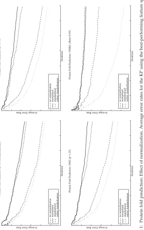
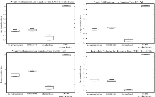
However, in online learning, where the full kernels are not observed be-forehand, methods 1 and 2 are clearly not possible, even where the explicit feature space is available (as in the case of linear kernels for example), since it requires the entire training set to be present. Since normalization is impor-tant for (most) multiple kernel methods, this poses a problem. Methods 3 to 5 are the only possibilities available, but they represent a weaker com-promise. Normalization or standardization in the input space clearly does not imply normalization or standardization in the feature space. However, it does represent a form of control over the vector sizes in the feature space and, as seen in the experimental section, does improve performance over no normalization.

The final method on the surface appears to make sense for linear kernels, as it should asymptotically converge to the standardization of the entire data set in the original space. We present experimental results for methods 3 to 5, as well as using no normalization.

Note also that it is possible to design online algorithms that automatically adapt to the norm of the samples observed up to any given time point. For example, Figures 5.2 and 5.3 of Shalev-Shwartz (2007) describe self-adaptive variants of the Winnow algorithm and aggressive quasi-additive family of algorithms, respectively, for binary classification. More recent approaches to solving this problem include an algorithm that adaptively chooses its regularization function based on the loss functions observed so far (McMahan & Streeter, 2010) and a new family of subgradient methods that dynamically incorporate the geometry of the data observed in earlier iterations to perform more informative gradient-based learning (Duchi, Hazan, & Singer, 2011). However, these methods are much more complex and are outside of the scope of this study.

8_{The restandardization of the active set can be ignored but will lead to poor}

4 Experiments

In this section, we present some empirical comparisons of a representative selection of the algorithms discussed earlier. In section 4.2, we present the analysis of a relatively small (in online learning terms) protein fold predic-tion data set. Due to the fact that multiple feature spaces are available, this data set has been used to benchmark and develop various different multiple kernel learning algorithms. Its compact nature allows us to rapidly evalu-ate a wide range of algorithms, discarding any that are too computationally expensive or show poor performance. Following on from this, we narrow down our selection of algorithms and analyze two object categorization data sets in section 4.3.

4.1 Algorithms and Specific Implementation Issues. This section lists

the algorithms we evaluated, along with any specific implementation is-sues that arose with these algorithms. All algorithms were implemented in Matlab version 7.7 (R2008b).

Since the data sets we are using have multiple feature spaces, they natu-rally lend themselves to the application of multiple kernel learning (MKL) algorithms. Note, however, that most of the algorithms presented here are single kernel algorithms. Of course we can create MKL algorithms from any of the single kernel algorithms by using ad hoc kernel combination rules. One such rule is simply to use an (unweighted) sum of kernels, which cor-responds to concatenating the feature spaces before creating a single kernel. Other kernel combinations could be used, such as products of kernels or nonlinear combinations of kernels, but these are outside the scope of this study. In order to do a complete analysis, ideally we would test each of the kernels separately using the single kernel methods as well as the ker-nel combinations. However, to keep the analysis contained, we treat the kernel perceptron (KP) as the benchmark algorithm. In doing so, we ran KP on each of the kernels separately, as well as with an unweighted sum of kernels (KP-sum). We then ran each of the single kernel methods using the unweighted sum in order to compare them with both KP-sum and the MKL methods. Of course, updating the kernel weights as well as the (dual) weight vectors in an online fashion is the ultimate goal, which at present only the OM-2 and OMKL methods attempt to do. Similar approaches could be taken to each of the single kernel methods, leading to many variants of online MKL, but that is outside of the scope of this work:

r

performing poorly (while this effectively turns this into the budget perceptron, this budget is not reached for any “useful” kernels).

r

variant, which throws away existing support vectors at random when the budget is exceeded. This method is seemingly naive but has good performance bounds and is extremely efficient. We used a maximum active set size of 200 samples.

r

DOGMA toolbox. The η (sparseness) parameter was set to its de-fault value. We found that the algorithm was very insensitive to this parameter.

r

de-fault is p= 1

1− 1

2 log(k). In the experiments that follow, this is

approxi-mately 1.25. We also tried the valuesp=1.01 andp=1.99 to approx-imate the ₁ and₂ norms (these will sometimes be referred to as

p=1 andp=2 for simplicity).

r

a discount (inverse sparsity) parameter 0< β <1. We used the set-tingsβ=0.1,0.5,0.9,0.99,0.999, since small values enforce sparsity over the kernel weights extremely quickly.

r

of 20 points (EP updates are performed only when 20 points are received). The buffer was chosen because if the initial EP did not include all of the classes, the future EP updates would never give posterior mass to those classes not included. We set the number of EP optimization iterations to 5.

r

window size to be the same as the IVM. Following Henao and Winther (2010), we set the inclusion parameter to 0.1, 0.3, and 0.6 and left the exclusion parameter at 0.99 after some experimenation.

Of course, we could have used any number of other possible choices of the various hyperparameters; these should be taken only as a representative sample rather than a definitive coverage of the various parameter spaces.

4.2 Protein Fold Prediction. The original data set from Ding and

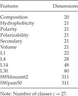
Table 2: Dimensionality of the Feature Spaces: Protein Fold Data.

Features Dimensions

Composition 20

Hydrophobicity 21

Polarity 21

Polarizability 21

Secondary 21

Volume 21

L1 22

L4 28

L14 48

L30 80

SWblosum62 311

SWpam50 311

Note: Number of classesc=27.

feature spaces in Ding and Dubchak (2001), the four proposed by Shen and Chou (2006) that describe pseudo–amino acid compositions (PseAA) estimated on different intervals of the protein sequence, and the two lo-cal alignment Smith-Waterman (SW)–based feature spaces, with different scoring matrices from Damoulas and Girolami (2008). The sizes of feature spaces are given in Table 2.

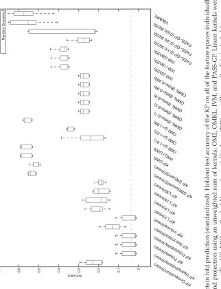
In order to calculate the holdout test accuracy, we stop the online algo-rithms after the first 313 examples have been seen and evaluate the resulting decision functions on the remaining 385 examples using the online-to-batch conversion described in section 1.1. To calculate the final cumulative accu-racy, we run the online algorithms through the whole data set (train and test) and calculate the number of online errors made during learning. Note that the two metrics therefore have different training set sizes.

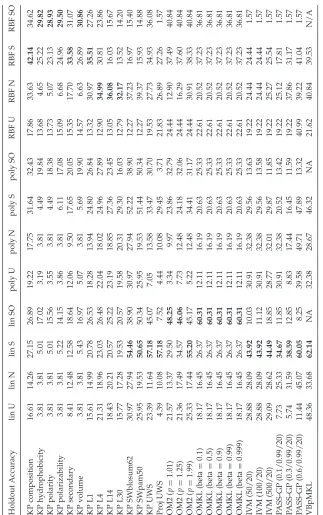
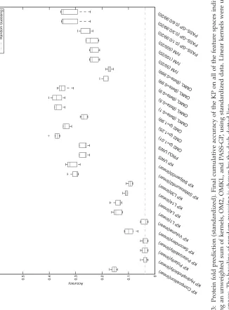
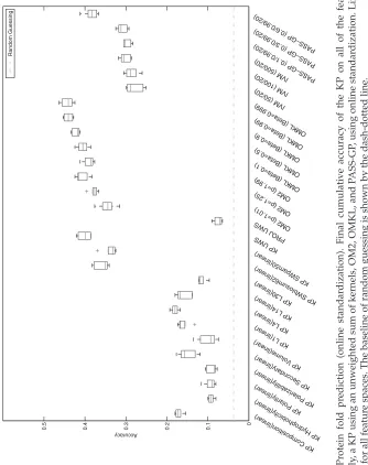
Tables 3 and 4 give holdout test accuracy and final cumulative (online) accuracy of the KP on all of the feature spaces individually, a KP using an unweighted sum of kernels, OM2, OMKL, and PASS-GP. In the columns are three kernel types:

r

r

lin-ear for local characteristics (SW) following Damoulas and Girolami (2008)

r

n as the width

parameter.9

9_{This is by no means optimal but serves as a simple heuristic method for choosing the}

The experiments were run using no normalization (lin U, poly/lin U, and RBF U), normalizing each example to be norm 1 (lin N, poly/lin N, RBF N), standardizing each example (lin S, poly/lin S, and RBF S), and online standardization (lin SO, poly/lin SO, and RBF SO). The results are reasonably consistent for both holdout test accuracy and cumulative accu-racy. For the KP on individual feature spaces, the RBF kernel performed best for all feature spaces except for the local characteristics (SW), where linear kernels performed best. In both cases, standardizing each example before computing kernels performed better than normalizing or no nor-malization. For KP on the unweighted sum of kernels, linear kernels on standardized data performed best under both metrics, and the same is true for the OM2 algorithm and PASS-GP. For OMKL, linear kernels on stan-dardized data were best in terms of cumulative accuracy, but RBF kernels on standardized data performed better in terms of holdout test accuracy.

The best method overall in terms of holdout test accuracy was the OMKL algorithm using linear kernels and the online standardization method (60.31%) for all values of the discount parameter β, followed closely by PASS-GP with the inclusion parameter at 0.6 (60.05%), both of which are close to the accuracy achived by the the variational Bayes probalistic mul-tiple kernel learning (VBpMKL) method of Damoulas and Girolami (2008) (an offline method), which was included for comparison (62.14%). For refer-ence, the KP and the projectron on the unweighted sum of kernels (KP UWS and Proj UWS) performed best using linear kernels on standardized data, and both achieved an accuracy of 57.18%; the OM2 followed behind this at 55.20%, withp=1.99. The best-performing single kernel was SWblosum62 (linear kernel, standardized) at 54.46%. The IVM performed worse than the best single kernel.

The best method overall in terms of cumulative test accuracy was again OMKL (β=0.999) with 44.31%, followed by OM2 with the least sparse setting (p=1.99) with 40.71% (both using linear kernels and the online standardization method). In terms of cumulative accuracy, KP UWS was close behind at 40.13%, and PASS-GP was further behind still (38.39%). The best single kernel was again SWblosum62 (linear kernel, online standard-ization). The projectron performed poorly according to this metric, as did the IVM.