http://go.warwick.ac.uk/lib-publications
Original citation:Khovanova, N. A., Khovanov, I. A., Sbano, L., Griffiths, F. and Holt, T. A.. (2012) Characterisation of linear predictability and non-stationarity of subcutaneous glucose profiles. Computer Methods and Programs in Biomedicine . (in press)
Permanent WRAP url:
http://wrap.warwick.ac.uk/52582 Copyright and reuse:
The Warwick Research Archive Portal (WRAP) makes the work of researchers of the University of Warwick available open access under the following conditions. Copyright © and all moral rights to the version of the paper presented here belong to the individual author(s) and/or other copyright owners. To the extent reasonable and practicable the material made available in WRAP has been checked for eligibility before being made available.
Copies of full items can be used for personal research or study, educational, or not-for-profit purposes without prior permission or charge. Provided that the authors, title and full bibliographic details are credited, a hyperlink and/or URL is given for the original metadata page and the content is not changed in any way.
Publisher’s statement:
“NOTICE: this is the author’s version of a work that was accepted for publication in Computer Methods and Programs in Biomedicine. Changes resulting from the publishing process, such as peer review, editing, corrections, structural formatting, and other quality control mechanisms may not be reflected in this document. Changes may have been made to this work since it was submitted for publication. A definitive version was subsequently published in Computer Methods and Programs in Biomedicine. http://dx.doi.org/10.1016/j.cmpb.2012.11.009
A note on versions:
The version presented here may differ from the published version or, version of record, if you wish to cite this item you are advised to consult the publisher’s version. Please see the ‘permanent WRAP url’ above for details on accessing the published version and note that access may require a subscription.
Characterization of Linear Predictability and Non-stationarity of Subcutaneous Glucose Profiles
N. A. Khovanova1, I. A. Khovanov1, L. Sbano2,3, F. Griffiths4,3, T.A. Holt5,4
1
School of Engineering, University of Warwick, Coventry, CV4 7AL, UK
2
Istituto Vincenzo Gioberti, Rome, 00153, Italy
3
Centre for Complexity Science, University of Warwick, Coventry, CV4 7AL, UK
4
Health Sciences Research Institute, University of Warwick, Coventry, CV4 7AL, UK
5
Department of Primary Care, University of Oxford, OX1 2ET, UK
Abstract—Continuous glucose monitoring is increasingly used in the management of diabetes.
Subcutaneous glucose profiles are characterized by a strong non-stationarity, which limits the
application of correlation-spectral analysis. We derived an index of linear predictability by
calculating the autocorrelation function of time series increments and applied detrended
fluctuation analysis to assess the non-stationarity of the profiles. Time series from volunteers
with both type 1 and type 2 diabetes and from control subjects were analysed. The results
suggest that in control subjects, blood glucose variation is relatively uncorrelated, and this
variation could be modelled as a random walk with no retention of ‘memory’ of previous values.
In diabetes, variation is both greater and smoother, with retention of inter-dependence between
neighboring values. Essential components for adequate longer term prediction were identified via
a decomposition of time series into a slow trend and responses to external stimuli. Implications
for diabetes management are discussed.
Keywords — Autocorrelation, Continuous glucose monitoring systems, Detrended fluctuation analysis, Diabetes Mellitus, Non-stationarity.
Corresponding author: Dr N. Khovanova, School of Engineering, University of Warwick,
Coventry, CV4 7AL, UK, Tel: +44(0)2476528242, Fax: +44(0)2476418922, e-mail:
I. INTRODUCTION
iabetes mellitus is a state of relative or absolute insulin deficiency, with or without insulin
resistance [1]. Insulin is the hormone that controls blood glucose levels (glycaemia), and
untreated diabetes is characterised by chronic hyperglycaemia (high levels of blood glucose).
Control of hyperglycaemia is important to prevent long term complications, including effects on
the eyes, kidneys, peripheral nerves, and cardiovascular system. Reduction of blood glucose
levels through both lifestyle and pharmacological interventions is the main therapeutic goal in
the management of diabetes. However, low levels (hypoglycaemia) are also dangerous, setting
patients and their clinicians a difficult challenge: the achievement and maintenance of glycaemic
stability.
People with diabetes are broadly categorised into ‘type 1’ and ‘type 2’. Individuals with type 1
become dependent on injected insulin at or soon after diagnosis and they have no tissue
resistance to insulin. For type 1 diabetes the artificial pancreas approach (automated closed loop
feedback between blood or subcutaneous glucose and insulin delivery) has attracted much
attention with significant progress but many remaining challenges [2]. ‘Type 2’ is typically
associated with obesity and insulin resistance, usually treatable without insulin but requiring
insulin in a proportion of patients. The rising global prevalence of type 2 diabetes, due both to
changes in lifestyle patterns and increasing life expectancy emphasizes the need for early
detection and intervention in individual patients. In contrast to type 1 diabetes (where the
artificial pancreas approach is of increasing interest), type 2 requires attention to the insulin
resistance element which can be modified by lifestyle changes as well as drug therapy.
Glycaemic stability requires a satisfactory mean glucose value, a reasonably narrow range
(typically between about 4.0 and 7 mmol L-1), and additionally, an adequate time horizon over
which blood glucose behaviour may be predicted into the future. This time horizon is related to
Understanding the interconnection of glucose values in a profile and the predictability of future
values are therefore important aspects of glycaemic control, enabling the individual to take
appropriate corrective action.
Glycosylated haemoglobin (HbA1c) is the most commonly used index to characterize
glycaemic control, and reflects average blood glucose values over 2-3 months [3]. However
patients with similar HbA1c values may display very different dynamical patterns. Therefore,
HbA1c is not an adequate measure of glycaemic stability and variability [3]. Determinants of
glycaemic variation include carbohydrate intake, exercise, insulin levels, insulin sensitivity, and
other factors.
Continuous monitoring [4] of subcutaneous glucose values taken every 3-5 minutes over
several days provides a detailed picture of glucose variability. Such profiles have been shown to
correlate well with blood glucose levels [3], although there is a lag between a change in blood
value (e.g. after food intake) and the response of the subcutaneous value [3, 5].
The main obstacles to statistical analysis are that subcutaneous glucose time series are
relatively short (few days), and their statistical characteristics demonstrate behaviour typical for
non-stationary processes [6]. As a result, certain measures including power spectrum and
autocorrelation function (ACF) [7, 8] are associated with significant errors and their use is
questionable [9]. The term stationarity/non-stationarity refers to the underlying process, not to a
particular realisation of it. Therefore, the property of ergodicity is usually assumed which
considers a single realization (time series) to be representative of the entire stochastic process [6,
7, 10]. In order to characterize these properties, however such a single time series must be much
longer than the longest characteristic time scale [6]. An obvious time scale in glucose profiles is
diurnal periodicity, therefore typically available 24-72 hour time series cannot be used to assess
the non-stationarity of the process in full. For such short realizations it is only possible to define
In this paper we consider glucose time-series as realizations of a non-stationary stochastic
process with stationary increments[7, 8, 10, 11]. This enables us to remove non-stationarity and
assess dynamical characteristics of the profiles. The aim is to develop descriptive non-parametric
tools that are universally applicable to characterize linear predictability in subcutaneous profiles
both of people with diabetes and controls. The non-stationarity itself is assessed through the use
of detrended fluctuation analysis (DFA) [12].
Recent studies have used techniques in the frequency domain to take the non-stationarity of
glucose profiles into account [13-15]. The Wigner-Ville distribution has been used [13] to
illustrate the difference in time-frequency patterns for 24-hour profiles of 4 diabetic patients and
1 control. The wavelet based time-scale distribution has been presented [14] for two non-diabetic
24-hour profiles with different meal regimens. An interesting parametric technique involving
frequency band decomposition and short-term forecasting using an autoregressive model has
been applied to the 72-hour profiles of nine type 1 diabetic patients [15]. We will consider a
non-parametric approach to assess data interconnections and predictability in thetimedomain.
DFA is a non-linear tool applicable to both stationary and non-stationary time series, and was
initially suggested to characterize so-called long range correlation for processes with algebraic
power-law ACF [12]: ), in the limit , i.e. when short-range correlation, for
example, exponential form )ex p() of ACF is not applicable [11, 16]. DFA leads to a
scaling index, , which is less than 1 for a stationary process and greater than 1 for
non-stationary [12]. Ogata et al [17] showed that DFA is able to discriminate healthy and diabetic
groups and they concluded that glucose profiles show negative long-range correlation for healthy
individuals and positive long-range correlation for diabetic patients (largely treated with insulin).
While this result and others [18] confirm the usefulness of DFA for characterizing the
a controversial issue [16]. We investigated the presence of long-range correlation in our glucose
profiles by verifying power-law scaling in the ACF of increments of time-series.
A different use of DFA for characterizing the amplitude of fluctuations versus diffusion
velocity of the non-stationary data has been suggested [19]. In this case, the value of is
compared with Brownian motion [19], an integrated white noise with uncorrelated increments
for which the DFA index is =1.5. Values of index 1 . 5 indicate the presence of a fast
fluctuating irregular component in the data, and 1 . 5 indicates the presence of a slower
stochastic component and stronger regularity.
Finally, we discuss possible origins and corresponding features of non-stationarity in glucose
dynamics as well as essential components for adequate longer term prediction by decomposing
the time series into the slow trend and meal time (prandial) events.
II. MATERIALS ANDMETHODS
A. Data Collection
We collected data from 15 volunteers, including patients with type 1 and type 2 diabetes, and
from controls with no diagnosis of diabetes. Recruitment was purposive to ensure a diverse
sample of ages and treatment regimens. Baseline biographical data were obtained on age, sex,
body mass index, type of diabetes, treatment regimen, and recent Hba1c value. Subcutaneous
glucose values were taken every five minutes over 72 hours using the Medtronic Minimed
CGMS (Continuous Glucose Monitoring System) [20]. Time series G(ti)=Gi are available for
each volunteer. Gi mmol L-1 is the glucose concentration at time moments ti=ih, where h=5
minutes is the sampling interval, i=1,2,…N and N specifies the length of time series. The
participants were asked to keep a diary recording the timing of food intake and exercise. No
B. Descriptive Statistics of Glucose Time-Series
Each individual was identified as type 1, type 2, or control (without diabetes) based on their
known diagnosis and treatment regimen. Continuous glucose monitoring gave us a detailed
picture of glucose variability and was used to derive various indices [21]. One of them - standard
deviation Gstdcharacterises the amplitude of glucose level fluctuations with respect to the mean
value, and has been used for diabetes diagnosis on basis of CGMS [21], although not in clinical
practice. We consider Gstd as a reference index and it was obtained using standard Matlab
functionstd.
The Mann Whitney U test (matlab function ranksum) was performed to assess whether data
from the different groups had similar values. The null hypothesis of no difference was tested [22]
at the 5% level of significance.
C. The Autocorrelation Function of Differential Increments
ACF is a function that characterises a linear statistical dependence (correlation) between
present and past values, defining a memory in the data [7, 8]. The strength of statistical
dependence specifies a probability of a given value in future taking into account the prehistory,
i.e. it reflects predictability. ACF has been applied to blood glucose time series [9, 23] to analyse
linear predictability, but as mentioned above, a major obstacle is the existence of non-stationary
behaviour.
To overcome the non-stationarity we considered each glucose profile as a realization of a
stochastic process with stationary increments [7, 8, 10, 11]. This approach is an established
technique for analysis of time series with a varying (non-stationary) mean value [7, 8]. However,
it is very rarely used for characterization of bio-medical data. Because the first difference is a
linear operation, the increments (and their ACF) preserve information about the trend. For
power-law scaling for long-range correlated processes will be observed in the ACFs of both
initial time-series and time-series of first-differences.
As the first step, the presence of a trend in the initial time series and the stationarity of
increments are confirmed via a corresponding statistical test of inversion [6], and by DFA. The
presence of the trend can also be demonstrated via a decomposition approach described below.
The second step involves representing the values from a glucose profile in the form Gi
GiGi, where differential increments Gi=Gi–Gi-1 correspond to the first differences of Gi,.
Since these incrementsGiare stationary, calculation of their ACF is straightforward.
ACF is defined by the following expression [6]
2
i mean i j mean j
std
X X X X
X
, (1)
where the bracketsmean time averaging, j=jh, j=0,1,2…,his the sampling period, andXiis
analysed time-series with mean value Xmean. This was calculated using the standard Matlab
functionxcorr. The resulting function j) belongs to the range [1:1]: values close to 1 suggest
a strong correlation between subsequent points separated by time interval (lag) j, and values
close to zero suggest an absence of correlations.
Exponential function (j)= exp(-j) was used to fit an initial decay of ACF and to
determine the ACF decay exponent . The initial decay relates to an interval ofj[0:30h]. The
exponent was then used to characterize the strength of correlation in the time series of
increments Gi. Smaller values of correspond to less rapid decay and hence stronger
D. Detrended Fluctuation Analysis
DFA exploits several parameters which can be varied and the choice of parameters
influences the final results and their interpretation. A detailed analysis of applicability of these
parameters and ways to interpret the DFA outputs are outside the scope of the current paper.
Here we follow an established numerical scheme [17]. A general calculation scheme for DFA
index has been published [12, 19] and the corresponding code is freely available [24]. This
involves scaling of detrended fluctuations of amplitudeF(n) as a function of window sizen:F(n)
n.
For a meaningful comparison between our results and those of Ogata et al [17], each glucose
profile was divided into non-overlapping 24 hour segments. This led to 15 segments for the
control group, and 13 and 12 segments for type 1 and type 2 diabetes groups respectively.
Following Ogata et al [17] the function F(n) was calculated for n[8:70] using a third order
detrending polynomial and overlapping windows. For some profiles there is a crossover point,
nc, where F(n) changes its scaling, and therefore two scaling indices 1 and 2 were used for
fitting:F(n)nfor short rangen[8:nc] andF(n)nfor long rangen[nc:70]. A minimum
of the error between piece-wise two-line fitting and F(n) has been used to determine the
crossover point nc. Thus, the outputs of the procedure are the presence/absence of the crossover
point and its location nc (if present); two scaling indices 1 and 2, which were considered as
equal if there was no crossover effect.
E. Trend Extraction
To consider long term prediction (usually defined as beyond one hour [4, 17]) and dynamic
behaviour, we decomposed the glucose time series into two parts. One part is a trend, and
another part corresponds to meal time (prandial) events. The data did not include an accurate
The trend was derived as a level connecting local minima and by taking into account the fact
that there is no food intake during night time. Prandial events can be considered as responses to
glucose intake and a number of mathematical models exist [25,26] for describing glucose-insulin
dynamics in such situations. A comprehensive discussion of the prandial events is beyond the
scope of this paper. The events were fitted for the purpose of illustration by the function
G(tte)=B1(exp[1(tte)]exp[2(tte)])-G(te), wheretecorresponds to the onset of the event, and
B1, 1 and 2 are constants. The first term is a particular solution of a linear second order
differential equation. This solution describes the impulse response of a linear system, i.e. a
response to an external perturbation changing G t( )e at a given time moment te. The solution
corresponds to a linearized version of a glucose homeostatic model recently suggested by
Watson et al [25]. Matlab function nlinfit, which performs nonlinear square regression, was used
for fitting.
III. RESULTS
A. Data collection and descriptive statistical analysis
The CGMS device was well tolerated with only minor problems reported, for instance keeping
the probe attached during very hot weather. In two cases the device was removed before
completing the 72 hours, but these nevertheless contained 648 and 674 consecutive glucose
measurements. There were no missing values in any of the profiles apart from profile 14, in
which there were difficulties with initial attachment of the monitoring system. Because this
interruption would have affected the analysis, the first 38 minutes of data were excluded prior to
an interlude of 19 minutes, still leaving a continuous series of 797 data points. In one participant
(profile 1) the device was kept on voluntarily (on the independent advice of the patient’s
The biographical data are given in Table 1. The 15 participants had a median age of 57 years,
range 22-74 years. Twelve were women. Five were controls with no diagnosis of diabetes, four
had type 1 diabetes and six had type 2. Two of the type 1 participants were using an insulin
pump; the other two were using a regimen of glargine (basal) and aspart (bolus) insulin
analogues. Of the six type 2 participants, one was using glargine in addition to metformin, all the
others were using oral medications only except for participant No 15, who was diagnosed with
diabetes at entry to the study and was not using any medication for diabetes. Hba1c
measurements ranged from 38 to 89mmol/mol, with median 53mmol/mol. The approximate
mapping [3] of HbA1c values to mean glucose level gives the range 6.3 to 13.8 mmol L-1with
median 8.5 mmol L-1.
TABLE 1
FIGURE 1.
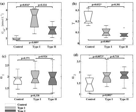
Figure 1 shows boxplots withp-values for calculated characteristics of all 15 profiles. If there is
a significant difference in medians between any two groups then the values are marked by a star.
It can be seen that standard deviation Gstd(Fig. 1, b) differs significantly between diabetes and
controls, as expected.
FIGURE 2.
B. ACF Analysis
Fig. 1, b shows box plots for ACF exponents, but before we discuss them, let us give an
illustration of ACF shapes and reaffirm the case for using the increments G(ti) instead of initial
time seriesG(ti) in the correlation analysis. In Figure 2,a, ACFs calculated for initial time series
component, related to diurnal activities, is clearly seen for glucose time-series G(ti), but not for
G(ti), where ACF has a non-oscillatory shape. Another example of ACF is shown in Figure 2, b
for a person from the control group (profile 3). In contrast to the first case, this graph does not
show a clear diurnal oscillatory component and the shape of ACF is typical for a long-range
correlation process. However ACF obtained using differential increments looks similar to the
diabetes case and both cases show fast decay to zero indicating only short-range memory. Let us
stress that a power-scaling in the case of long-range correlation must be observed for both the
initial data G(ti), and for increments G(ti) [11]. Therefore, these two pictures demonstrate the
absence of long-range memory. This demonstrates the limitations of using ACF for analysis of
time-series G(ti) and its applicability to increments G(ti). However, if the focus of interest is
specifically to identify periodicities, then spectral analysis [13, 14] of the original time series
may also be useful.
The box plots shown in Fig. 1, b demonstrate that ACF exponent is smaller in the diabetic
groups, indicating stronger correlation of data with time, and higher in the control group
indicating uncorrelated dynamics.
C. Detrended Fluctuation analysis
The DFA indices and (Fig. 1, c, and d) are greater than1 for all profiles indicating the
presence of non-stationary behaviour in the time series.
The crossover effect has been observed in most of the segments (39 out of 47). The index1
for the short range is not statistically different (Fig. 1, c), whereas the index 2 is statistically
different for control and diabetes groups (Fig. 1, d). For a comparison to the previous
investigation by Ogata et al [17], results of both type 1 and type 2 diabetes groups were
Ogata et al [17] gave the following results: 1=1.77±0.32, 2=1.25±0.29 for the control group;
1=1.72±0.21, 2=1.65±0.30 for the diabetes group. Our results are the following:
1=1.84±0.23, 2=1.44±0.30 for the control group; 1=1.95±0.36, 2=1.83±0.31 for the
combined diabetes group. There is a qualitative correspondence between these two investigations
since both show that the difference is not significant for 1 (p=0.278 for our data) but it is
significant for 2(p=0.0004 for our data). However, values of indices1 and2for our data are
larger than in Ogata et al’s study [17]. Several factors may explain this difference. Their
participants were asked to follow certain prescriptions for food intake, refraining from all forms
of caffeine, limitations on physical activity and scheduled times to wake up and go to sleep. Our
participants had no such restrictions. Perhaps more importantly, fourteen of their fifteen
participants with diabetes were using insulin. Our sample included more diverse treatment
regimens: five using insulin, four using tablet treatment alone, and one using neither (Table 1).
Index2as already mentioned is significantly different for control and diabetic groups. The
value of 2 is close to 1.5 for controls which in combination with the ACF index, allows us to
present the dynamics as a random walk with independent increments, i.e. as Brownian motion.
For diabetic groups,2is higher than 1.5, suggesting a slow variation of the corresponding time
series.
FIGURE 3.
D. Glucose Variation as a Stochastic Process
Thus, ACF exponent DFA index and standard deviation all show clear differences between
control and diabetes groups. Figure 3 suggests monotonic nonlinear dependences between the 3
parameters meaning that any one of them is sufficient for differentiation between the diabetes
reflect different properties of the glucose profiles: linear predictability (), non-stationary
behaviour () and amplitude of variation (Gstd). Interestingly, the combination of two indices,
Gstd and leads to a two-dimensional map (Fig. 3, a). Here, indices of control and diabetic
groups form distinct clusters with a hypothetical boundary represented by a dashed line whereas
we see overlap of values if only one of the indices is considered at a time (Fig 1 and Fig 3),
particularly for.
FIGURE 4.
E. Decomposition and Trend Extraction
Figure 4 demonstrates the presence of prandial excursions in the profiles (two profiles for type
2 diabetes are shown as examples) superimposed on a slow component, a trend, and this is
typical for all our time series. There are no clear regular patterns in the slow components and the
predictability of the trends is an open question.
In each profile several peaks corresponding to prandial events were chosen and fitted (red thin
lines in Figure 4) as described in the Methods section. The fit in the form of the impulse response
of a linear system works well for all control cases, however it gives inconsistent results for
diabetic time series of both type 1 and type 2. In our example in Figure 4 the fit is good forabut
poor for b: peaks in a have an asymmetric shape, whereas peaks are more symmetrical in b.
Values of the fitting coefficients vary from peak to peak for each profile indicating a strong
nonlinear dependence on the amplitude of external stimuli. Therefore, for the control group and
for some of the participants with diabetes the response to food intake can be effectively modelled
by a second order linear equation, however specific non-linear and/or high dimensional models
IV. DISCUSSION
A. Summary of Principal Findings
Our results suggest that subcutaneous glucose variation can be modeled as a stochastic process
with stationary increments. ACF analysis of the increments indicates the presence of short-range
memory using an exponential decay function for ACF fitting. Long-range trends in the original
glucose profiles are removed effectively by this technique, enabling comparison between
diabetic and control profiles, and the value of DFA is confirmed.
We found that 3 characteristics (standard deviationGstd, ACF exponent and DFA index
differentiate between control and diabetic groups, and uniquely define independent properties of
the glucose profiles. These complementary parameters suggest that in the control state, blood
glucose variations are small in amplitude and relatively uncorrelated over time scales of 10 to 20
minutes, during which ACF decays rapidly. These variations could be modelled as a random
walk, with no retention of ‘memory’ of previous values, i.e. Brownian motion. In diabetes, by
contrast, variation is greater in amplitude and smoother, with retention of inter-dependence
between neighbouring values in a profile; ACF decays less abruptly, suggesting persistence of
correlated structure over short time scales of 30 minutes to one hour. ACF exponent is shown
to be a qualitative indicator of linear predictability.
Our use of increments rather than the original time series enables us to compare the glucose
dynamics of both healthy individuals and diabetic patients. Further natural extension of this
technique is an application ofspectralanalysis and probability measures of the increments.
The decomposition of time series to the slow trend related to intrinsic dynamics and responses
to external stimuli has demonstrated an event-driven character of glucose variation, highlighting
the importance of explicit inclusion of external stimuli into prediction models, as is used in
artificial pancreas systems [2]. Additionally, it suggests that long term predictions (beyond one
well with a previously published finding [4] that the use of short time windows can support
simple auto-regressive models for short-term forecasting [4, 23]. Longer term prediction may
require a better understanding of the slow trend. For some time series the trend can be
represented by an oscillatory function related to a diurnal component, but for most of the profiles
in our study a clear diurnal periodicity was absent.
B. Limitations of the Study
This is an exploratory study investigating the potential for time series analysis to support a
dynamical definition of glycaemic stability. It is inevitably limited by the relatively small sample
of profiles available, but has confirmed the ability of such data to support this approach in the
clinical setting. A larger study would involve more participants preferably using a broader range
of therapies including different insulin replacement regimens, as well as newer anti-diabetic
agents such as GLP-1 analogues, which were not included in our study. This would identify the
effects of different therapies on the glucose dynamics. Longer time series (over weeks or months
rather than days) would allow the detection of longer term patterns (including weekly and
monthly periodicities [28]) but are more difficult to collect unless the sampling frequency is
significantly reduced or new technologies emerge [29].
ACKNOWLEDGMENT
This work was supported in part by EPSRC (EP/C53932X/2). The study was approved by
Coventry Local Research Ethics Committee reference 06/Q2802/1. We thank Rachel Potter for
gathering the data using the CGMS device.
REFERENCES
[1] L. Poretsky (Ed.), Principles of Diabetes Mellitus, 2nd Ed (New York: Springer 2010).
[2] R. Hovorka, Closed-loop insulin delivery: from bench to clinical practice, Nat. Rev.
[3] D. M. Nathan, J. Kuenen, R. Borg, H. Zheng, D. Schoenfeld, R. J. Heine, and for the
A1c-Derived Average Glucose (ADAG) Study Group, Translating the A1C Assay Into Estimated
Average Glucose Values, Diabetes Care 31 (2008) 1473-1478.
[4] G. Sparacino, A. Facchinetti and C. Cobelli, Smart continuous glucose monitoring sensors:
On-line signal processing issues, Sensors,10 (2010) 6751-6772.
[5] K. Sikaris, The correlation of hemoglobin A1c to blood glucose, J. Diabetes Sci. Technol. 3
(2009) 429-438.
[6] J.S. Bendat and A. G. Piersol, Random Data: Analysis and Measurement Procedures, (New
York; Chichester: Wiley, 1986).
[7] S. M. Rytov, Y. A. Kravtsov and V. I. Tatarskii, Principles of Statistical Radiophysics, Vol.
2, Correlation Theory of Random Processes, (Berlin: Springer, 1988).
[8] A. M. Yaglom, An Introduction to the Theory of Stationary Random Functions, (Englewood
Cliffs, NJ: Prentice-Hall, 1962).
[9] T. Bremer and D. A. Gough, Is blood glucose predictable from previous values? A
solicitation for data, Diabetes 48 (1999) 445-451.
[10] N. A. Khovanova, I. A. Khovanov, Methods of analysis of time series. (Saratov. Izdatelstvo
GosUNC "Kolledg", 2001, in Russian).
[11] I. I Eliazar and M. F. Shlesinger, Langevin unification of fractional motions, J. Phys. A:
Math. Theor. 45 (2012) 162002.
[12] C. K. Peng, S. Havlin, H. E. Stanley and A. L. Goldberger, Quantification of scaling
exponents and crossover phenomena in nonstationary heartbeat time series, Chaos 5 (1995) 82–
87.
[13] I. Iancu, M. Mota and E. Iancu, Method for the analysing of blood glucose dynamics in
diabetes mellitus patients, in Automation, Quality and Testing, Robotics, 2008. AQTR 2008.
[14] F. N. Rahaghi and D. A. Gough, Blood glucose dynamics, Diabetes Technol. Ther. 10
(2008) 81-94.
[15] Y. Lu, A. Gribok, K. Ward and J. Reifman, The importance of different frequency bands in
predicting subcutaneous glucose concentration in type 1 diabetic patients, IEEE Trans. Biomed.
Eng. 57 (2010) 1839-1846.
[16] D. Maraun, H. W. Rust and J. Timmer, Tempting long-memory – on the interpretation of
DFA results, Nonlinear Processes in Geophysics, 11 (2004) 495-503.
[17] H. Ogata, K. Tokuyama, S. Nagasaka, A. Ando, I. Kusaka, N. Sato, A. Goto, S. Ishibashi,
K. Kiyono, Z. R. Struzik and Y. Yamamoto, Long-range negative correlation of glucose
dynamics in humans and its breakdown in diabetes mellitus, Am. J. Physiol. Regul. Integr.
Comp. Physiol., 291 (2006) R1638–R1643.
[18] J. Churruca, L. Vigil, E. Luna, J. Ruiz-Galiana, M. Varela, The route to diabetes: Loss of
complexity in the glycemic profile from health through the metabolic syndrome to type 2
diabetes, Diabetes, Metabolic Syndrome and Obesity 1 (2008) 3–11.
[19] I. A. Khovanov, N. A. Khovanova, P. V. E. McClintock and A. Stefanovska, Intrinsic
dynamics of heart regulatory systems on short time-scales: from experiment to modeling, J. Stat.
Mech. (2009) p01016.
[20] B. Wilhelm, S. Forst, M. M. Weber, M. Larbig, A. Pfutzner, T. Forst, Evaluation of CGMS
during rapid blood glucose changes in patients with type 1 diabetes, Diabetes Technol. Ther., 8
(2006) 146-155.
[21] L. Monnier, C. Colette and D. R. Owens, Glycemic variability: The third component of the
dysglycemia in diabetes. Is it important? How to measure it? J. Diabetes Sci. Technol. 2, (2008)
1094-1100.
[23] A. Gani, A. V. Gribok, S. Rajaraman, W. K. Ward and J. Reifman, Predicting subcutaneous
glucose concentration in humans: data-driven glucose modeling, IEEE Trans. Biomed. Eng. 56
(2009) 246-254.
[24] PHYSIONET web site athttp://www.physionet.org/physiotools/dfa/
[25] E. M. Watson, M. J. Chappell, F. Ducrozet, S. M. Poucher, J. W. T. Yates, A new general
glucose homeostatic model using a proportional-integral-derivative controller, Computer
Methods and Programs in Biomedicine 102 (2011) 119-129.
[26] R. Burattini and M. Morettini, Identification of an integrated mathematical model of
standard oral glucose tolerance test for characterization of insulin potentiation in health,
Computer Methods and Programs in Biomedicine 107 (2012) 248-261.
[27] A. Duggento, D. G. Luchinsky, V. N. Smelyanskiy, I. Khovanov and P. V. McClintock,
Inferential framework for nonstationary dynamics. II. Application to a model of physiological
signaling, Phys. Rev. E 77 (2008) 061106.
[28] J. J. Liszka-Hackzell, Prediction of blood glucose levels in diabetic patients using a hybrid
AI technique, Comput. Biomed. Res. 32 (1999) 132-144.
[29] N. S. Oliver, C. Toumazou, A. E. G. Cass, D. G. Johnston, Glucose sensors: a review of
approximate glucose levels [3] of participants
Profile
No.
Age
(years)
Sex BMI
(kg/m2)
Diabetes
status
Treatment regimen HbA1c
(mmol/mol)
Glucose level
(mmol L-1)
1 57 F 20.5 Type 1 Basal bolus (glargine
plus aspart)
63 10.0
2 27 F 19.2 Control N/A N/A N/A
3 59 F 27.3 Control N/A N/A N/A
4 49 F 21.9 Control N/A N/A N/A
5 32 F 29.4 Type 1 Insulin pump 55 9.0
6 74 M 20.5 Type 2 Metformin, gliclazide
and rosiglitazone
61 9.7
7 66 F 25.9 Type 1 Insulin pump 38 6.3
8 75 M 23.4 Type 2 Metformin 46 7.6
9 68 F 32.7 Type 1 Basal bolus (glargine
plus aspart)
48 7.8
10 39 F 21.3 Control N/A N/A N/A
11 61 F 32.6 Type 2 Metformin 52 8.4
12 56 M 30.0 Type 2 Metformin and gliclazide 68 10.8
13 52 F 44.5 Type 2 Metformin and glargine 89 13.8
14 22 F 19.6 Control N/A N/A
15 63 F 27.0 Type 2 Newly diagnosed diet
only
[image:20.595.69.582.135.709.2]3). The solid blue and dashed red lines correspond to ACF calculated for time series G(ti) and
[image:22.595.81.483.23.603.2]Gstd(x-axis) versus DFA index,cACF decay exponent,(x-axis) versus DFA indexThe
results are shown by green circles, red squares and blue pluses for the control, type1 and type 2
groups respectively. Dash-dot lines show boundaries for one parametric analysis; the dashed line
group. The solid thick black line corresponds to the trend; measured glucose values are shown by
circles; fitting curves are shown by thin red lines. The dashed and solid vertical lines correspond
[image:24.595.105.484.34.563.2]