Attention is not Explanation

Proceedings of NAACL-HLT 2019, pages 3543–3556 3543

Attention is not Explanation

Sarthak Jain

Northeastern University

[email protected]

Byron C. Wallace

Northeastern University

[email protected]

Abstract

Attention mechanisms have seen wide adop-tion in neural NLP models. In addition to improving predictive performance, these are often touted as affording transparency: mod-els equipped with attention provide a distribu-tion over attended-to input units, and this is often presented (at least implicitly) as com-municating the relative importance of inputs. However, it is unclear what relationship ex-ists between attention weights and model out-puts. In this work we perform extensive exper-iments across a variety of NLP tasks that aim to assess the degree to which attention weights provide meaningful “explanations" for predic-tions. We find that they largely do not. For example, learned attention weights are fre-quently uncorrelated with gradient-based mea-sures of feature importance, and one can iden-tify very different attention distributions that nonetheless yield equivalent predictions. Our findings show that standard attention mod-ules do not provide meaningful explanations and should not be treated as though they do. Code to reproduce all experiments is avail-able athttps://github.com/successar/

AttentionExplanation.

1 Introduction and Motivation

Attention mechanisms(Bahdanau et al.,2014) in-duce conditional distributions over input units to compose a weighted context vector for down-stream modules. These are now a near-ubiquitous component of neural NLP architectures. Attention weights are often claimed (implicitly or explic-itly) to afford insights into the “inner-workings” of models: for a given output one can inspect the inputs to which the model assigned large attention weights. Li et al. (2016) summarized this com-monly held view in NLP: “Attention provides an important way to explain the workings of neural models". Indeed, claims that attention provides

after 15 minutes watching the movie i was asking myself what to do leave the theater sleep or try to keep watching the movie to see if there was anything worth i finally watched the movie what a waste of time maybe i am not a 5 years old kid anymore

original adversarial after 15 minutes watching the movie i was asking myself what to do leave the theater sleep or try to keep watching the movie to see if there was anything worth i finally watched the movie what a waste of time maybe i am not a 5 years old kid anymore

f(x|↵, ✓) = 0.01 f(x|↵, ✓˜ ) = 0.01

↵ ↵˜

Figure 1: Heatmap of attention weights induced over a negative movie review. We show observed model tention (left) and an adversarially constructed set of at-tention weights (right). Despite being quite dissimilar, these both yield effectively the same prediction (0.01).

interpretability are common in the literature, e.g., (Xu et al.,2015;Choi et al.,2016;Lei et al.,2017;

Martins and Astudillo,2016;Xie et al.,2017).1 Implicit in this is the assumption that the input units (e.g., words) accorded high attention weights are responsible for model outputs. But as far as we are aware, this assumption has not been for-mally evaluated, and our findings here suggest that it is problematic. More specifically, we empir-ically investigate the relationship between atten-tion weights, inputs, and outputs. Assuming at-tention provides an explanation for model predic-tions, we might expect the following properties to hold. (i) Attention weights should correlate with feature importance measures (e.g., gradient-based measures); (ii) Alternative (orcounterfactual) at-tention weight configurations ought to yield corre-sponding changes in prediction (and if they do not then are equally plausible as explanations). We re-port that neither property is consistently observed by standard attention mechanisms in the context of text classification, question answering (QA), and Natural Language Inference (NLI) tasks when RNN encoders are used.

Consider Figure 1. The left panel shows the original attention distributionαover the words of a particular movie review using a standard atten-tive BiLSTM architecture for sentiment analysis. It is tempting to conclude from this that the token

wasteis largely responsible for the model coming to its disposition of ‘negative’ (yˆ= 0.01). But one can construct an alternative attention distribution

˜

α(right panel) that attends to entirely different to-kens yet yields an essentially identical prediction (holding all other parameters off,θ, constant).

Such counterfactual distributions imply that ex-plaining the original prediction by highlighting attended-to tokens is misleading insofar as alter-native attention distributions would have yielded an equivalent prediction (e.g., one might conclude from the right panel that model output was due pri-marily towasrather than waste). Further, the at-tention weights in this case correlate only weakly with gradient-based measures of feature impor-tance (τg = 0.29). And arbitrarily permuting the

entries in α yields a median output difference of 0.006 with the original prediction.

These and similar findings call into question the view that attention provides meaningful insight into model predictions. We thus caution against using attention weights to highlight input tokens “responsible for” model outputs and constructing just-so stories on this basis, particularly with com-plex encoders.

Research questions and contributions. We ex-amine the extent to which the (often implicit) nar-rative that attention provides modeltransparency2

holds across tasks by exploring the following em-pirical questions.

1. To what extent do induced attention weights correlate with measures of feature impor-tance – specifically, those resulting from gra-dients andleave-one-outmethods?

2. Would alternative attention weights (and hence distinct heatmaps/“explanations”) nec-essarily yield different predictions?

Our findings with respect to these questions (as-suming a BiRNN encoder) are summarized as fol-lows: (1) Only weakly and inconsistently, and, (2) No; it is very often possible to construct adver-sarialattention distributions that yield effectively

2_{Defined as per (Lipton, 2016); we are interested in} whether attended-to features are responsible for outputs.

equivalent predictions as when using the origi-nally induced attention weights, despite attending to entirely different input features. Further, ran-domly permuting attention weights often induces only minimal changes in output.

2 Preliminaries and Assumptions

We consider exemplar NLP tasks for which atten-tion mechanisms are commonly used: classifica-tion, natural language inference (NLI), and ques-tion answering.3 We adopt the following general modeling assumptions and notation.

We assume model inputs x ∈ RT×|V|,

com-posed of one-hot encoded words at each position.

These are passed through an embedding matrixE

which provides dense (ddimensional) token repre-sentationsxe∈RT×d. Next, an encoderEnc

con-sumes the embedded tokens in order, producing T m-dimensional hidden states: h = Enc(xe) ∈

RT×m. We predominantly consider a Bi-RNN

as the encoder module, but for completeness we also analyze convolutional and (unordered) ‘aver-age embedding’ variants.4

A similarity function φ maps h and a query

Q∈Rm(e.g., hidden representation of a question

in QA, or the hypothesis in NLI) to scalar scores, and attention is then induced over these: αˆ =

softmax(φ(h,Q)) ∈ RT. In this work we

con-sider two common similarity functions: Additive φ(h,Q) = vTtanh(W1h +W2Q) (Bahdanau et al., 2014) andScaled Dot-Product φ(h,Q) =

hQ √

m (Vaswani et al.,2017), wherev,W1,W2are

model parameters.

Finally, a dense layer Dec with parameters θ

consumes a weighted instance representation and yields a predictionyˆ = σ(θ·hα) ∈ R|Y|, where hα =PTt=1αˆt·ht;σis an output activation

func-tion; and|Y|denotes the label set size.

3 Datasets and Tasks

Forbinary text classification, we use:

Stanford Sentiment Treebank (SST) (Socher et al.,2013). 10,662 sentences tagged with senti-ment on a scale from 1 (most negative) to 5 (most positive). We filter out neutral instances and di-chotomize the remaining sentences into positive (4, 5) and negative (1, 2).

3_{While attention is perhaps most common in seq2seq} tasks like translation, our impression is that interpretability is not typically emphasized for such tasks, in general.

4_{In the latter case,h}

Dataset |V| Avg. length Train size Test size Test performance

SST 16175 19 3034 / 3321 863 / 862 0.81

IMDB 13916 179 12500 / 12500 2184 / 2172 0.88

ADR Tweets 8686 20 14446 / 1939 3636 / 487 0.61

20 Newsgroups 8853 115 716 / 710 151 / 183 0.94

AG News 14752 36 30000 / 30000 1900 / 1900 0.96

Diabetes (MIMIC) 22316 1858 6381 / 1353 1295 / 319 0.79

Anemia (MIMIC) 19743 2188 1847 / 3251 460 / 802 0.92

CNN 74790 761 380298 3198 0.64

bAbI (Task 1 / 2 / 3) 40 8 / 67 / 421 10000 1000 1.0 / 0.65 / 0.64

SNLI 20982 14 182764 / 183187 / 183416 3219 / 3237 / 3368 0.78

Table 1: Dataset characteristics. For train and test size, we list the cardinality for each class, where applicable:

0/1for binary classification (top), and 0 / 1 / 2 for NLI (bottom). Average length is in tokens. Test metrics are F1 score, accuracy, and micro-F1 for classification, QA, and NLI, respectively; all correspond to performance using a BiLSTM encoder. We note that results using convolutional and average (i.e., non-recurrent) encoders are comparable for classification though markedly worse for QA tasks.

IMDB Large Movie Reviews Corpus (Maas et al., 2011). Binary sentiment classification dataset containing 50,000 polarized (positive or negative) movie reviews, split into half for train-ing and testtrain-ing.

Twitter Adverse Drug Reactiondataset ( Nikfar-jam et al., 2015). A corpus of ∼8000 tweets re-trieved from Twitter, annotated by domain experts as mentioning adverse drug reactions.

20 Newsgroups (Hockey vs Baseball).

Col-lection of ∼20,000 newsgroup correspondences,

partitioned (nearly) evenly across 20 categories.

We extract instances belonging to baseball and

hockey, which we designate as 0 and 1, respec-tively, to derive a binary classification task.

AG News Corpus (Business vs World).5496,835

news articles from 2000+ sources. We follow

(Zhang et al.,2015) in filtering out all but the top 4 categories. We consider the binary classification task of discriminating betweenworld(0) and busi-ness(1) articles.

MIMIC ICD9 (Diabetes)(Johnson et al.,2016). A subset of discharge summaries from the MIMIC III dataset of electronic health records. The task is to recognize if a given summary has been labeled with the ICD9 code for diabetes (or not).

MIMIC ICD9 (Chronic vs Acute Anemia)( John-son et al., 2016). A subset of discharge sum-maries from MIMIC III dataset (Johnson et al.,

2016) known to correspond to patients with mia. Here the task to distinguish the type of ane-mia for each report –acute(0) orchronic(1).

ForQuestion Answering (QA):

CNN News Articles (Hermann et al., 2015). A corpus of cloze-style questions created via

auto-5_{http://www.di.unipi.it/~gulli/AG_}

corpus_of_news_articles.html

matic parsing of news articles from CNN. Each instance comprises a paragraph-question-answer triplet, where the answer is one of the anonymized entities in the paragraph.

bAbI (Weston et al., 2015). We consider the three tasks presented in the original bAbI dataset paper, training separate models for each. These entail finding (i) a single supporting fact for a question and (ii) two or (iii) three supporting state-ments, chained together to compose a coherent line of reasoning.

Finally, forNatural Language Inference(NLI):

TheSNLI dataset(Bowman et al.,2015). 570k human-written English sentence pairs manually labeled for balanced classification with the labels

neutral,contradiction, andentailment, supporting the task of natural language inference (NLI). In this work, we generate an attention distribution over premise words conditioned on the hidden rep-resentation induced for the hypothesis.

We restrict ourselves to comparatively sim-ple instantiations of attention mechanisms, as de-scribed in the preceding section. This means we do not consider recently proposed ‘BiAttentive’ architectures that attend to tokens in the respec-tive inputs, conditioned on the other inputs (Parikh et al.,2016;Seo et al.,2016;Xiong et al.,2016).

Table 1 provides summary statistics for all

datasets, as well as the observed test performances for additional context.

4 Experiments

We run a battery of experiments that aim to ex-amine empirical properties of learned attention weights and to interrogate their interpretability

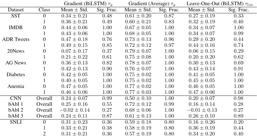
Gradient (BiLSTM)τg Gradient (Average)τg Leave-One-Out (BiLSTM)τloo Dataset Class Mean±Std. Sig. Frac. Mean±Std. Sig. Frac. Mean±Std. Sig. Frac.

SST 0 0.34±0.21 0.48 0.61±0.20 0.87 0.27±0.19 0.33 1 0.36±0.21 0.49 0.60±0.21 0.83 0.32±0.19 0.40 IMDB 0 0.44±0.06 1.00 0.67±0.05 1.00 0.34±0.07 1.00 1 0.43±0.06 1.00 0.68±0.05 1.00 0.34±0.07 0.99 ADR Tweets 0 0.47±0.18 0.76 0.73±0.13 0.96 0.29±0.20 0.44 1 0.49±0.15 0.85 0.72±0.12 0.97 0.44±0.16 0.74 20News 0 0.07±0.17 0.37 0.79±0.07 1.00 0.06±0.15 0.29 1 0.21±0.22 0.61 0.75±0.08 1.00 0.20±0.20 0.62 AG News 0 0.36±0.13 0.82 0.78±0.07 1.00 0.30±0.13 0.69 1 0.42±0.13 0.90 0.76±0.07 1.00 0.43±0.14 0.91 Diabetes 0 0.42±0.05 1.00 0.75±0.02 1.00 0.41±0.05 1.00 1 0.40±0.05 1.00 0.75±0.02 1.00 0.45±0.05 1.00 Anemia 0 0.47±0.05 1.00 0.77±0.02 1.00 0.46±0.05 1.00 1 0.46±0.06 1.00 0.77±0.03 1.00 0.47±0.06 1.00 CNN Overall 0.24±0.07 0.99 0.50±0.10 1.00 0.20±0.07 0.98 bAbI 1 Overall 0.25±0.16 0.55 0.72±0.12 0.99 0.16±0.14 0.28 bAbI 2 Overall −0.02±0.14 0.27 0.68±0.06 1.00 −0.01±0.13 0.27 bAbI 3 Overall 0.24±0.11 0.87 0.61±0.13 1.00 0.26±0.10 0.89 SNLI 0 0.31±0.23 0.36 0.59±0.18 0.80 0.16±0.26 0.20 1 0.33±0.21 0.38 0.58±0.19 0.80 0.36±0.19 0.44 2 0.31±0.21 0.36 0.57±0.19 0.80 0.34±0.20 0.40

Table 2: Mean and std. dev. of correlations between gradient/leave-one-out importance measures and attention weights. Sig. Frac. columns report the fraction of instances for which this correlation is statistically significant; note that this largely depends on input length, as correlation does tend to exist, just weakly. Encoders are denoted parenthetically. These are representative results; exhaustive results for all encoders are available to browse online.

learned attention weights agree with alternative, natural measures of feature importance? And,

Had we attended to different features, would the prediction have been different?

More specifically, in Section 4.1, we empir-ically analyze the correlation between gradient-based feature importance and learned attention weights, and between ‘leave-one-out’ (LOO) mea-sures and the same. In Section4.2 we then con-sider counterfactual (to those observed) attention distributions. Under the assumption that atten-tion weights are explanatory, such counterfactual distributions may be viewed as alternative poten-tial explanations; if these do not correspondingly change model output, then the original attention weights do not provide unique explanation for predictions, i.e., attending to other features could have resulted in the same output.

To generate counterfactual attention distribu-tions, we first consider randomly permuting ob-served attention weights and recording associated changes in model outputs (4.2.1). We then pro-pose explicitly searching for “adversarial” atten-tion weights that maximally differ from the ob-served attention weights (which one might show in a heatmap and use to explain a model prediction), and yet yield an effectively equivalent prediction (4.2.2). The latter strategy also provides a use-ful potential metric for the reliability of attention weights as explanations: we can report a measure

quantifying how different attention weights can be for a given instance without changing the model output by more than some threshold.

All results presented below are generated on test sets. We present results for Additive

atten-tion below. The results for Scaled Dot Product

in its place are comparable. We provide a web interface to interactively browse the (very large set of) plots for all datasets, model variants, and

experiment types: https://successar.github.

io/AttentionExplanation/docs/.

In the following sections, we use Total Vari-ation Distance (TVD) as the measure of change between output distributions, defined as follows. TVD(ˆy1,yˆ2) = 1₂P

|Y|

i=1|yˆ1i − yˆ2i|. We use

the Jensen-Shannon Divergence (JSD) to quan-tify the difference between two attention dis-tributions: JSD(α1, α2) = 1₂KL[α1||α1+₂α2] +

1

2KL[α2||

α1+α2

2 ].

4.1 Correlation Between Attention and Feature Importance Measures

We empirically characterize the relationship be-tween attention weights and corresponding fea-ture importance scores. Specifically we measure correlations between attention and: (1) gradient based measures of feature importance (τg), and,

(2) differences in model output induced by leav-ing features out (τloo). While these measures are

neu-1.0 0.5 0.0 0.5 1.0 0.000

0.025 0.050 0.075 0.100 0.125

(a) SST (BiLSTM)

1.0 0.5 0.0 0.5 1.0 0.000

0.025 0.050 0.075 0.100 0.125 0.150

(b) SST (Average)

1.0 0.5 0.0 0.5 1.0 0.0

0.1 0.2 0.3 0.4 0.5 0.6

(c) Diabetes (BiLSTM)

1.0 0.5 0.0 0.5 1.0 0.0

0.2 0.4 0.6 0.8

(d) Diabetes (Average)

1 0 1

0.000 0.025 0.050 0.075 0.100 0.125

1 0 1

0.00 0.05 0.10 0.15

0.0 0.2 0.4 0.6 0.8 1.0 0.0

0.2 0.4 0.6 0.8 1.0

(e) SNLI (BiLSTM)

1 0 1

0.0 0.1 0.2 0.3

1 0 1

0.00 0.05 0.10 0.15

0.0 0.2 0.4 0.6 0.8 1.0 0.0

0.2 0.4 0.6 0.8 1.0

(f) SNLI (Average)

1 0 1

0.00 0.05 0.10 0.15 0.20 0.25 0.30

1 0 1

0.0 0.1 0.2 0.3

0.0 0.2 0.4 0.6 0.8 1.0 0.0

0.2 0.4 0.6 0.8 1.0

(g) CNN-QA (BiLSTM)

1 0 1

0.00 0.05 0.10 0.15

1 0 1

0.00 0.05 0.10 0.15 0.20

0.0 0.2 0.4 0.6 0.8 1.0 0.0

0.2 0.4 0.6 0.8 1.0

(h) BAbI 1 (BiLSTM)

Figure 2: Histogram of Kendallτ between attention and gradients. Encoder variants are denoted parenthetically; colors indicate predicted classes. Exhaustive results are available for perusal online. Best viewed in color.

ral model behavior (Feng et al., 2018), they do provide measures of individual feature importance with known semantics (Ross et al.,2017). It is thus instructive to ask whether these measures correlate with attention weights.

The process we follow to quantify this is de-scribed in Algorithm1. We denote the input re-sulting from removing the word at positiontinx

byx−t. Note that we disconnect the computation

graph at the attention module so that the gradient does not flow through this layer.

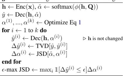
Algorithm 1Feature Importance Computations

h_←Enc(x),αˆ _←softmax(φ(h,Q)) ˆ

y _←Dec(h, α)

gt← |P

|V|

w=11[xtw= 1]_∂∂y_xtw|,∀t∈[1, T] τg←Kendall-τ(α, g)

∆ˆyt←TVD(ˆy(x−t),yˆ(x)),∀t∈[1, T] τloo←Kendall-τ(α,∆ˆy)

Table 2 reports summary statistics of Kendall τ correlations for each dataset. Full distributions are shown inFigure 2, which plots histograms of τg for every data point in the respective corpora.

(Corresponding plots for τloo are similar and the

full set can be browsed via the online supplement.) We plot these separately for each class: orange () represents instances predicted as positive, and pur-ple () those predicted to be negative. For SNLI, colors,andcode for contradiction, entail-ment, and neutral respectively.

In general, observed correlations are modest

(recall: 0 indicates no correspondence, 1

im-plies perfect concordance) for the BiRNN encoder. The centrality of observed densities hovers around or below 0.5 in most of the corpora considered. Moreover, as per Table2, correlation is sufficiently weak that a statistically significant correlation be-tween attention weights and feature importance scores (both gradient and feature erasure based) cannot consistently be established across corpora.

In contrast, gradients in “average” embedding based models show very high degree of correspon-dence with attention weights – on average across corpora, correlation between LOO scores and at-tention weights is ∼0.375 points higher for this encoder, compared to the BiLSTM. These results suggest that, in general, attention weights do not strongly or consistently agree with such feature importance scores in models with contextualized embeddings. This is problematic for the view of attention weights as explanatory, given the face validity of input gradient/erasure based explana-tions (Ross et al.,2017;Li et al.,2016). On some datasets — notably the MIMIC tasks, and to a lesser extent the QA corpora — this correlation is consistently significant but remains relatively weak. This could be attributed to increased length of documents for these datasets providing stronger signal to standard hypothesis testing methods.

either feature importance score for the recurrent (BiLSTM) encoder. These exhibit, on average, a (i)0.2and (ii)_∼0.25greater correlation with each other than BiLSTM attention and (i) LOO and (ii) gradient scores.

4.2 Counterfactual Attention Weights

We next considerwhat-if scenarios corresponding to alternative (counterfactual) attention weights. The idea is to investigate whether the prediction would have been different, had the model empha-sized (attended to) different input features. More precisely, suppose αˆ = _{αˆt}Tt=1 are the atten-tion weights induced for an instance, giving rise to model outputyˆ. We then consider counterfac-tual distributions overy, under alternativeα.

We experiment with two means of construct-ing such distributions. First, we simply scram-ble the original attention weights αˆ, re-assigning each value to an arbitrary, randomly sampled in-dex (input feature). Second, we generate an ad-versarial attention distribution: this is a set of at-tention weights that is maximally distinct fromαˆ

but that nonetheless yields an equivalent predic-tion (i.e., predicpredic-tion within someofyˆ).

4.2.1 Attention Permutation

To characterize model behavior when attention weights are shuffled, we follow Algorithm2.

Algorithm 2Permuting attention weights

h_←Enc(x),αˆ _←softmax(φ(h,Q)) ˆ

y _←Dec(h,αˆ)

forp←1to100do αp _{←Permute(ˆα)}

ˆ

yp_{←Dec(h, α}p_{) .Note :his not changed}

∆ˆyp _←TVD[ˆyp_,yˆ] end for

∆ˆymed_←Median

p(∆ˆyp)

Figure 3 depicts the relationship between the maximum attention value in the originalαˆand the median induced change in model output (∆ˆymed₎

across instances in the respective datasets. Colors again indicate class predictions, as above.

We observe that there exist many points with small ∆ˆymed _{despite large magnitude attention}

weights. These are cases in which the attention weights might suggest explaining an output by a small set of features (this is how one might reasonably read a heatmap depicting the atten-tion weights), but where scrambling the attenatten-tion

makes little difference to the prediction.

In some cases, such as predicting ICD codes from notes using the MIMIC dataset, one can see different behavior for the respective classes. For the Diabetes task, e.g., attention behaves intu-itively for at least the positive class; perturbing attention in this case causes large changes to the prediction. We again conjecture that this is due to a few tokens serving as high precision indicators for the positive class; in their absence (or when they are not attended to sufficiently), the predic-tion drops considerably. However, this is the ex-ception rather than the rule.

4.2.2 Adversarial Attention

We next propose a more focused approach to counterfactual attention weights, which we will re-fer to asadversarial attention. The intuition is to explicitly seek out attention weights that differ as much as possible from the observed attention dis-tribution and yet leave the prediction effectively unchanged. Such adversarial weights violate an intuitive property of explanations: shifting model attention to very different input features should yield corresponding changes in the output. Alter-native attention distributions identified adversari-ally may then be viewed as equadversari-ally plausible ex-planations for the same output.

Operationally, realizing this objective requires specifying a valuethat defines what qualifies as a “small” difference in model output. Once this is specified, we aim to find k adversarial distri-butions{α(1)_{, ..., α}(k)_{}, such that eachα}(i) max-imizes the distance from original αˆ but does not change the output by more than. In practice we simply set this to0.01 for text classification and

0.05for QA datasets.6

We propose the following optimization problem to identify adversarial attention weights.

maximize

α(1)_,...,α(k) f({α

(i)_}k

i=1)

subject to ∀iTVD[ˆy(x, α(i)),yˆ(x,αˆ)]≤ (1)

Wheref(_{α(i)_}k i=1)is:

k X

i=1

JSD[α(i),αˆ] + 1

k(k₋1)

X

i<j

JSD[α(i), α(j)]

(2)

0.0 0.5 1.0 Median Output Difference [0.00,_0.25)

[0.25, 0.50) [0.50, 0.75) [0.75, 1.00)

Max attention

(a) SST (BiLSTM)

0.0 0.5 1.0

Median Output Difference [0.00,_0.25)

[0.25, 0.50) [0.50, 0.75) [0.75, 1.00)

Max attention

(b) SST (CNN)

0.0 0.5 1.0

[0.00,_0.25)

[0.25, 0.50) [0.50, 0.75) [0.75, 1.00)

(c) Diabetes (BiLSTM)

0.0 0.5 1.0

[0.00,_0.25)

[0.25, 0.50) [0.50, 0.75) [0.75, 1.00)

(d) Diabetes (CNN)

0.0 0.5 1.0

[0.00, 0.25) [0.25,_0.50)

[0.50, 0.75) [0.75,_1.00)

(e) CNN-QA (BiLSTM)

0.0 0.5 1.0

[0.00, 0.25) [0.25,_0.50)

[0.50, 0.75) [0.75,_1.00)

(f) bAbI 1 (BiLSTM)

0.0 0.5 1.0

[0.00, 0.25) [0.25,_0.50)

[0.50, 0.75) [0.75,_1.00)

(g) SNLI (BiLSTM)

0.0 0.5 1.0

[0.00, 0.25) [0.25,_0.50)

[0.50, 0.75) [0.75,_1.00)

(h) SNLI (CNN)

Figure 3: Median change in output (∆ˆymed_{) (x-axis) densities in relation to the max attention (max ˆα) (y-axis)} obtained by randomly permuting instance attention weights. Encoders denoted parenthetically. Plots for all corpora and using all encoders are available online.

In practice we maximize a relaxed version of this objective via the Adam SGD opti-mizer (Kingma and Ba, 2014): f({α(i)_}k

i=1) + λ

k

Pk

i=1max(0,TVD[ˆy(x, α(i)),yˆ(x,αˆ)]−).7 Equation1attempts to identify a set of new at-tention distributions over the input that is as far

as possible from the observed α (as measured

by JSD) and from each other (and thus diverse),

while keeping the output of the model within

of the original prediction. We denote the

out-put obtained under theith_{adversarial attention by}

ˆ

y(i)_{. Note that the JS Divergence between any two} categorical distributions (irrespective of length) is bounded from above by 0.69.

One can view an attentive decoder as a func-tion that maps from the space of latent input repre-sentations and attention weights over input words

∆T−1 _{to a distribution over the output space Y.} Thus, for any outputyˆ, we can define how likely each attention distributionαwill generate the out-put as inversely proportional to TVD(y(α),yˆ).

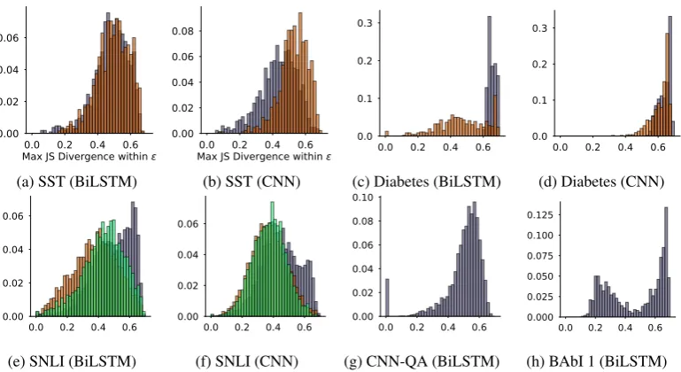
Figure 4 depicts the distributions of max JSDs realized over instances with adversarial attention weights for a subset of the datasets considered. Colors again indicate predicted class. Mass toward the upper-bound of 0.69 indicates that we are fre-quently able to identify maximally different atten-tion weights that hardly budge model output. We observe that one can identify adversarial attention weights associated with high JSD for a significant number of examples. This means that is often the

7_{We setλ= 500.}

Algorithm 3Finding adversarial attention weights

h_←Enc(x),αˆ ←softmax(φ(h,Q)) ˆ

y←Dec(h,αˆ)

α(1)_{, ..., α}(k) _{←Optimize Eq1} fori←1tokdo

ˆ

y(i)_{←Dec(h, α}(i)_{) .his not changed}

∆ˆy(i) _{←TVD[ˆy,yˆ}(i)_]

∆α(i)_{←JSD[ˆα, α}(i)_] end for

-max JSD_←maxi1[∆ˆy(i)≤]∆α(i)

case that quite different attention distributions over inputs would yield essentially the same (within) output.

In the case of the diabetestask, we again ob-serve a pattern of low JSD for positive examples (where evidence is present) and high JSD for neg-ative examples. In other words, for this task, if one perturbs the attention weights when it is inferred that the patient is diabetic, this does change the output, which is intuitively agreeable. However, this behavior again is an exception to the rule.

0.0 0.2 0.4 0.6 Max JS Divergence within 0.00

0.02 0.04 0.06

0.0 0.2 0.4 0.6 Max JS Divergence within [0.00, 0.25) [0.25, 0.50) [0.50, 0.75) [0.75, 1.00) Max Attention

(a) SST (BiLSTM)

0.0 0.2 0.4 0.6 Max JS Divergence within 0.00

0.02 0.04 0.06 0.08

0.0 0.2 0.4 0.6 Max JS Divergence within [0.00, 0.25) [0.25, 0.50) [0.50, 0.75) [0.75, 1.00) Max Attention

(b) SST (CNN)

0.0 0.2 0.4 0.6 0.0

0.1 0.2 0.3

0.0 0.2 0.4 0.6 Max JS Divergence within [0.00, 0.25) [0.25, 0.50) [0.50, 0.75) [0.75, 1.00) Max Attention

(c) Diabetes (BiLSTM)

0.0 0.2 0.4 0.6 0.0

0.1 0.2 0.3

0.0 0.2 0.4 0.6 Max JS Divergence within [0.00, 0.25) [0.25, 0.50) [0.50, 0.75) [0.75, 1.00) Max Attention

(d) Diabetes (CNN)

0.0 0.2 0.4 0.6 0.00

0.02 0.04 0.06

0.0 0.2 0.4 0.6 Max Attention [0.00, 0.25) [0.25, 0.50) [0.50, 0.75) [0.75, 1.00) Ma x J S Di ve rg en ce w ith in

(e) SNLI (BiLSTM)

0.0 0.2 0.4 0.6 0.00

0.02 0.04 0.06

0.0 0.2 0.4 0.6 Max Attention [0.00, 0.25) [0.25, 0.50) [0.50, 0.75) [0.75, 1.00) Ma x J S Di ve rg en ce w ith in

(f) SNLI (CNN)

0.0 0.2 0.4 0.6 0.00 0.02 0.04 0.06 0.08 0.10

0.0 0.2 0.4 0.6 Max Attention [0.00, 0.25) [0.25, 0.50) [0.50, 0.75) [0.75, 1.00) Ma x J S Di ve rg en ce w ith in

(g) CNN-QA (BiLSTM)

0.0 0.2 0.4 0.6 0.000 0.025 0.050 0.075 0.100 0.125

0.0 0.2 0.4 0.6 Max Attention [0.00, 0.25) [0.25, 0.50) [0.50,_0.75) [0.75, 1.00) Ma x J S Di ve rg en ce w ith in

(h) BAbI 1 (BiLSTM)

Figure 4: Histogram of maximum adversarial JS Divergence (-max JSD) between original and adversarial atten-tions over all instances. In all cases shown,_|yˆadv

−yˆ_|< . Encoders are specified in parantheses. Best viewed in color.

would be more difficult to identify.

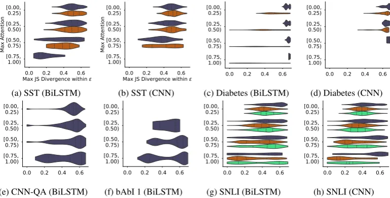
Figure 5 illustrates that while there is a nega-tive trend to this effect, it is realized only weakly. Put another way: there exist many cases (in all datasets) in which despite a high attention weight, an alternative and quite different attention config-uration over inputs yields effectively the same out-put. In light of this, presenting a heatmap implying that a particular set of features is primarily respon-sible for an output would seem to be misleading.

5 Related Work

We have focused on attention mechanisms and the question of whether they afford transparency, but a number of interesting strategies unrelated to atten-tion mechanisms have been recently proposed to provide insights into neural NLP models. These include approaches that measure feature impor-tance based on gradient information (Ross et al.,

2017;Sundararajan et al.,2017) (aligned with the gradient-based measures that we have used here), and methods based on representation erasure(Li et al., 2016), in which dimensions are removed and then the resultant change in output is recorded (similar to our experiments with removing tokens from inputs, albeit we do this at the input layer).

Comparing such importance measures to atten-tion scores may provide addiatten-tional insights into the working of attention based models (Ghaeini et al., 2018). Another novel line of work in this direction involves explicitly identifying explana-tions of black-box predicexplana-tions via a causal

frame-work (Alvarez-Melis and Jaakkola, 2017). We

also note that there has been complementary work demonstrating correlation between human atten-tion and induced attenatten-tion weights, which was rel-atively strong when humans agreed on an explana-tion (Pappas and Popescu-Belis, 2016). It would be interesting to explore if such cases present plicit ‘high precision’ signals in the text (for ex-ample, the positive label in diabetes dataset).

More specific to attention mechanisms, re-cent promising work has proposed more princi-pled attention variants designed explicitly for in-terpretability; these may provide greater trans-parency by imposinghard,sparseattention. Such instantiations explicitly select (modest) subsets of inputs to be considered when making a predic-tion, which are then by construction responsible for model output (Lei et al., 2016; Peters et al.,

2018). Structured attention models (Kim et al.,

2017) provide a generalized framework for

de-scribing and fitting attention variants with explicit probabilistic semantics. Tying attention weights to human-provided rationales is another potentially promising avenue (Bao et al., 2018). We hope our work motivates further development of these methods, resulting in attention variants that both improve predictive performance and provide in-sights into model predictions.

6 Discussion and Conclusions

(in-0.0 0.2 0.4 0.6 Max JS Divergence within 0.00

0.02 0.04 0.06

0.0 0.2 0.4 0.6 Max JS Divergence within [0.00, 0.25) [0.25, 0.50) [0.50, 0.75) [0.75, 1.00) Max Attention

(a) SST (BiLSTM)

0.0 0.2 0.4 0.6 Max JS Divergence within 0.00 0.02 0.04 0.06 0.08 0.10

0.0 0.2 0.4 0.6 Max JS Divergence within [0.00, 0.25) [0.25, 0.50) [0.50, 0.75) [0.75, 1.00) Max Attention

(b) SST (CNN)

0.0 0.2 0.4 0.6 0.0

0.1 0.2 0.3

0.0 0.2 0.4 0.6 [0.00, 0.25) [0.25, 0.50) [0.50, 0.75) [0.75, 1.00)

(c) Diabetes (BiLSTM)

0.0 0.2 0.4 0.6 0.0

0.1 0.2 0.3

0.0 0.2 0.4 0.6 [0.00, 0.25) [0.25, 0.50) [0.50, 0.75) [0.75, 1.00)

(d) Diabetes (CNN)

0.0 0.2 0.4 0.6 0.00 0.02 0.04 0.06 0.08 0.10

0.0 0.2 0.4 0.6 [0.00, 0.25) [0.25, 0.50) [0.50,_0.75) [0.75, 1.00)

(e) CNN-QA (BiLSTM)

0.0 0.2 0.4 0.6 0.000 0.025 0.050 0.075 0.100 0.125

0.0 0.2 0.4 0.6 [0.00, 0.25) [0.25, 0.50) [0.50, 0.75) [0.75,_1.00)

(f) bAbI 1 (BiLSTM)

0.0 0.2 0.4 0.6 0.00

0.02 0.04 0.06

0.0 0.2 0.4 0.6 [0.00, 0.25) [0.25, 0.50) [0.50,_0.75) [0.75, 1.00)

(g) SNLI (BiLSTM)

0.0 0.2 0.4 0.6 0.00

0.02 0.04 0.06

0.0 0.2 0.4 0.6 [0.00, 0.25) [0.25, 0.50) [0.50,_0.75) [0.75, 1.00)

(h) SNLI (CNN)

Figure 5: Densities of maximum JS divergences (-max JSD) (x-axis) as a function of the max attention (y-axis) in each instance for obtained between original and adversarial attention weights.

cluding gradient and feature erasure approaches) and learned attention weights is weak when using

a BiRNN encoder (Section 4.1). We also

estab-lished that counterfactual attention distributions — which would tell a different story about why a model made the prediction that it did — often have no effect on model output (Section4.2).

These results suggest that while attention mod-ules consistently yield improved performance on NLP tasks, their ability to provide transparency for model predictions is (in the sense of point-ing to inputs responsible for outputs) questionable. More generally, how one is meant to interpret the ‘heatmaps’ of attention weights placed over inputs that are commonly presented is unclear. These seem to suggest a story about how a model arrived at a particular disposition, but the results here in-dicate that the relationship between this and atten-tion is not obvious, at least for RNN encoders.

There are important limitations to this work

and the conclusions we can draw from it. We have reported the (generally weak) correlation between learned attention weights and various alternative measures of feature importance, e.g., gradients. We do not imply that such alternative measures are necessarily ideal or should be considered ‘ground truth’. While such measures do enjoy a clear in-trinsic (to the model) semantics, their interpreta-tion for non-linear neural networks can nonethe-less be difficult for humans (Feng et al., 2018). Still, that attention consistently correlates poorly withmultiplesuch measures ought to give pause to practitioners. That said, exactly how strong such correlations ‘should’ be to establish reliability as

explanation is an admittedly subjective question. We note that the counterfactual attention ex-periments demonstrate the existence of alternative heatmaps that yield equivalent predictions; thus one cannot conclude that the model made a partic-ular predictionbecauseit attended over inputs in a specific way. But these adversarial weights may themselves be unlikely under the attention module parameters. Further, it may be that multiple plau-sible explanations exist, complicating interpreta-tion. We would maintain that in such cases the model should highlight all plausible explanations, but one may instead view a model that provides ‘sufficient’ explanation as reasonable.

An additional limitation is that we have only considered a handful of attention variants, selected to reflect common module architectures for the respective tasks included in our analysis. Alter-native attention specifications may yield different conclusions; and indeed we hope this work moti-vates further development of principled attention mechanisms (or encoders). Finally, we have lim-ited our evaluation to tasks with unstructured out-put spaces, i.e., we have not considered seq2seq tasks, which we leave for future work. However we believe interpretability is more often a consid-eration in, e.g., classification than in translation.

Acknowledgements

We thank Zachary Lipton for insightful feedback on a preliminary version of this manuscript.

References

David Alvarez-Melis and Tommi S Jaakkola. 2017. A causal framework for explaining the predictions of black-box sequence-to-sequence models. arXiv preprint arXiv:1707.01943.

Dzmitry Bahdanau, Kyunghyun Cho, and Yoshua Ben-gio. 2014. Neural machine translation by jointly learning to align and translate. arXiv preprint arXiv:1409.0473.

Yujia Bao, Shiyu Chang, Mo Yu, and Regina Barzilay. 2018. Deriving machine attention from human ra-tionales. arXiv preprint arXiv:1808.09367.

Samuel R Bowman, Gabor Angeli, Christopher Potts, and Christopher D Manning. 2015. A large anno-tated corpus for learning natural language inference. arXiv preprint arXiv:1508.05326.

Edward Choi, Mohammad Taha Bahadori, Jimeng Sun, Joshua Kulas, Andy Schuetz, and Walter Stewart. 2016. Retain: An interpretable predictive model for healthcare using reverse time attention mechanism. InAdvances in Neural Information Processing Sys-tems, pages 3504–3512.

Shi Feng, Eric Wallace, Alvin Grissom II, Pedro Rodriguez, Mohit Iyyer, and Jordan Boyd-Graber. 2018. Pathologies of neural models make interpreta-tion difficult. InEmpirical Methods in Natural Lan-guage Processing.

Reza Ghaeini, Xiaoli Fern, and Prasad Tadepalli. 2018. Interpreting recurrent and attention-based neural models: a case study on natural language inference. In Proceedings of the 2018 Conference on Empiri-cal Methods in Natural Language Processing, pages 4952–4957.

Karl Moritz Hermann, Tomas Kocisky, Edward Grefenstette, Lasse Espeholt, Will Kay, Mustafa Su-leyman, and Phil Blunsom. 2015. Teaching ma-chines to read and comprehend. InAdvances in Neu-ral Information Processing Systems, pages 1693– 1701.

Alistair EW Johnson, Tom J Pollard, Lu Shen, H Lehman Li-wei, Mengling Feng, Moham-mad Ghassemi, Benjamin Moody, Peter Szolovits, Leo Anthony Celi, and Roger G Mark. 2016. Mimic-iii, a freely accessible critical care database. Scientific data, 3:160035.

Yoon Kim, Carl Denton, Luong Hoang, and Alexan-der M Rush. 2017. Structured attention networks. arXiv preprint arXiv:1702.00887.

Diederik P Kingma and Jimmy Ba. 2014. Adam: A method for stochastic optimization. arXiv preprint arXiv:1412.6980.

Tao Lei, Regina Barzilay, and Tommi Jaakkola. 2016. Rationalizing neural predictions. arXiv preprint arXiv:1606.04155.

Tao Lei et al. 2017. Interpretable neural models for natural language processing. Ph.D. thesis, Mas-sachusetts Institute of Technology.

Jiwei Li, Will Monroe, and Dan Jurafsky. 2016. Un-derstanding neural networks through representation erasure. arXiv preprint arXiv:1612.08220.

Zachary C Lipton. 2016. The mythos of model inter-pretability. arXiv preprint arXiv:1606.03490.

Andrew L. Maas, Raymond E. Daly, Peter T. Pham, Dan Huang, Andrew Y. Ng, and Christopher Potts. 2011. Learning word vectors for sentiment analy-sis. InProceedings of the 49th Annual Meeting of the Association for Computational Linguistics: Hu-man Language Technologies, pages 142–150, Port-land, Oregon, USA. Association for Computational Linguistics.

Andre Martins and Ramon Astudillo. 2016. From soft-max to sparsesoft-max: A sparse model of attention and multi-label classification. In International Confer-ence on Machine Learning, pages 1614–1623.

Azadeh Nikfarjam, Abeed Sarker, Karen Oâ ˘A ´ ZCon-nor, Rachel Ginn, and Graciela Gonzalez. 2015.

Pharmacovigilance from social media: mining ad-verse drug reaction mentions using sequence

label-ing with word embeddlabel-ing cluster features. Journal

of the American Medical Informatics Association, 22(3):671–681.

Nikolaos Pappas and Andrei Popescu-Belis. 2016. Hu-man versus machine attention in document classifi-cation: A dataset with crowdsourced annotations. In Proceedings of The Fourth International Workshop on Natural Language Processing for Social Media, pages 94–100.

Ankur P Parikh, Oscar Täckström, Dipanjan Das, and Jakob Uszkoreit. 2016. A decomposable attention model for natural language inference. arXiv preprint arXiv:1606.01933.

Ben Peters, Vlad Niculae, and André FT Martins. 2018. Interpretable structure induction via sparse atten-tion. InProceedings of the 2018 EMNLP Workshop BlackboxNLP: Analyzing and Interpreting Neural Networks for NLP, pages 365–367.

Andrew Slavin Ross, Michael C Hughes, and Finale Doshi-Velez. 2017. Right for the right reasons: Training differentiable models by constraining their explanations. arXiv preprint arXiv:1703.03717.

Minjoon Seo, Aniruddha Kembhavi, Ali Farhadi, and Hannaneh Hajishirzi. 2016. Bidirectional attention flow for machine comprehension. arXiv preprint arXiv:1611.01603.

empirical methods in natural language processing, pages 1631–1642.

Mukund Sundararajan, Ankur Taly, and Qiqi Yan. 2017. Axiomatic attribution for deep networks. arXiv preprint arXiv:1703.01365.

Ashish Vaswani, Noam Shazeer, Niki Parmar, Jakob Uszkoreit, Llion Jones, Aidan N Gomez, Łukasz Kaiser, and Illia Polosukhin. 2017. Attention is all you need. InAdvances in Neural Information Pro-cessing Systems, pages 5998–6008.

Jason Weston, Antoine Bordes, Sumit Chopra, Alexan-der M Rush, Bart van Merriënboer, Armand Joulin, and Tomas Mikolov. 2015. Towards ai-complete question answering: A set of prerequisite toy tasks. arXiv preprint arXiv:1502.05698.

Qizhe Xie, Xuezhe Ma, Zihang Dai, and Eduard Hovy. 2017. An interpretable knowledge transfer model for knowledge base completion. arXiv preprint arXiv:1704.05908.

Caiming Xiong, Victor Zhong, and Richard Socher. 2016. Dynamic coattention networks for question answering. arXiv preprint arXiv:1611.01604.

Kelvin Xu, Jimmy Ba, Ryan Kiros, Kyunghyun Cho, Aaron Courville, Ruslan Salakhudinov, Rich Zemel, and Yoshua Bengio. 2015. Show, attend and tell: Neural image caption generation with visual at-tention. In International Conference on Machine Learning, pages 2048–2057.

Xiang Zhang, Junbo Zhao, and Yann LeCun. 2015. Character-level convolutional networks for text clas-sification. In Advances in neural information pro-cessing systems, pages 649–657.

Ye Zhang, Iain Marshall, and Byron C Wallace. 2016. Rationale-augmented convolutional neural networks for text classification. InProceedings of the Con-ference on Empirical Methods in Natural Language Processing (EMNLP), volume 2016, pages 795–804.

Appendices

A Model details

For all datasets, we use spaCy for tokenization. We map out of vocabulary words to a special

<unk> token and map all words with numeric characters to ‘qqq’. Each word in the vocabulary was initialized to pretrained embeddings. For gen-eral domain corpora we used either (i) FastText Embeddings (SST, IMDB, 20News, and CNN) trained on Simple English Wikipedia, or, (ii)

GloVe 840B embeddings (AGNews and SNLI). For the MIMIC dataset, we learned word embed-dings usingGensimover all discharge summaries

in the corpus. We initialize words not present

in the vocabulary using samples from a standard Gaussian_N(µ= 0,σ2 _{= 1).}

A.1 BiLSTM

We use an embedding size of 300 and hidden size of 128 for all datasets except bAbI (for which we use 50 and 30, respectively). All models were reg-ularized using `2 regularization (λ = 10−5) ap-plied to all parameters. We use a sigmoid activa-tion funcactiva-tions for binary classificaactiva-tion tasks, and a softmax for all other outputs. We trained the model using maximum likelihood loss using the Adam Optimizer with default parameters in Py-Torch.

A.2 CNN

We use an embedding size of 300 and 4 kernels of sizes [1, 3, 5, 7], each with 64 filters, giving a final hidden size of 256 (for bAbI we use 50 and 8 re-spectively with same kernel sizes). We use ReLU activation function on the output of the filters. All other configurations remain same as BiLSTM.

A.3 Average

We use the embedding size of 300 and a projection size of 256 with ReLU activation on the output of the projection matrix. All other configurations re-main same as BiLSTM.

B Further details regarding attentional module of gradient

In the gradient experiments, we made the decision to cut-off the computation graph at the attention module so that gradient does not flow through this layer and contribute to the gradient feature im-portance score. For the sake of gradient calcula-tion this effectively treats the attencalcula-tion as a sepa-rate input to the network, independent of the input. We argue that this is a natural choice to make for our analysis because it calculates:how much does the output change as we perturb particular inputs (words) by a small amount, while paying the same amount of attention to said word as originally es-timated and shown in the heatmap?

C Correlations between Feature Importance measures

A question one might have here is how well cor-related LOO and gradients are withone another. We report such results in their entirety on the pa-per website, and we summarize their correlations relative to those realized by attention in a

BiL-STM model with LOO measures in Figure6. This

0.1 0.0 0.1 0.2 0.3 0.4

Mean Difference between Correlations

SST IMDB ADR AG News 20 News Sports Diabetes Anemia CNN bAbI 1 bAbI 2 bAbI 3 SNLI

Dataset

Figure 6: Mean difference in correlation of (i) LOO vs. Gradients and (ii) Attention vs. LOO scores using BiLSTM Encoder + Tanh Attention. On average the former is more correlated than the latter by>0.2τloo.

0.0 0.1 0.2 0.3 0.4

Mean Difference between Correlations

SST IMDB ADR AG News 20 News Sports Diabetes Anemia CNN bAbI 1 bAbI 2 bAbI 3 SNLI

Dataset

Figure 7: Mean difference in correlation of (i) LOO vs. Gradients and (ii) Attention vs. Gradients using BiLSTM Encoder + Tanh Attention. On average the former is more correlated than the latter by_∼0.25τg.

and LOO correlations, and (ii) attention and LOO correlations. As expected, we find that these ex-hibit, in general, considerably higher correlation with one another (on average) than LOO does with attention scores. (The lone exception is on SNLI.) Figure7 shows the same for gradients and atten-tion scores; the differences are comparable. In the

ADRand Diabetescorpora, a few high precision tokens indicate (the positive) class, and in these cases we see better agreement between LOO/gra-dient measures with attention; this is consistent with Figure4 which shows that it is difficult for the BiLSTM variant to find adversarial attention distributions forDiabetes.

A potential issues with using Kendallτ as our metric here is that (potentially many) irrelevant features may add noise to the correlation mea-sures. We acknowledge that this as a shortcoming of the metric. One observation that may mitigate this concern is that we might expect such noise to depress the LOO and gradient correlations to the same extent as they do the correlation between

at-0.0 0.1 0.2 0.3 0.4 0.5 0.6 0.7

Mean Difference between Correlations

SST IMDB ADR AG News 20 News Sports Diabetes Anemia CNN bAbI 1 bAbI 2 bAbI 3 SNLI

Dataset

Figure 8: Difference in mean correlation of attention weights vs. LOO importance measures for (i) Av-erage (feed-forward projection) and (ii) BiLSTM En-coders with Tanh attention. Average correlation (ver-tical bar) is on average _∼0.375 points higher for the simple feedforward encoder, indicating greater corre-spondence with the LOO measure.

tention and feature importance scores; but as per Figure7, they do not. We also note that the cor-relations between the attention weights on top of feedforward (projection) encoder and LOO scores are much stronger, on average, than those be-tween BiLSTM attention weights and LOO. This is shown in Figure8. Were low correlations due simply to noise, we would not expect this.8

D Graphs

To provide easy navigation of our (large set

of) graphs depicting attention weights on

various datasets/tasks under various model

configuration we have created an interactive interface to browse these results, accessible

at: https://successar.github.io/

AttentionExplanation/docs/.

E Adversarial Heatmaps

SST

Original: reggio falls victim to relying on the very digital technology that he fervently scorns creating a meandering inarticulate and ultimately disappointing film

Adversarial: reggio falls victim to relying on the very digital technology that he fervently scorns creating a meandering inarticulate and ultimately disappointing film∆ˆy:0.005

IMDB

Original: fantastic movie one of the best film noir movies ever made bad guys bad girls a jewel heist a twisted morality a kidnapping everything is here jean has a face that would make bogart proud and the rest of the cast is is full of character actors who seem to to know they’re onto something good get some popcorn and have a great time

Adversarial: fantastic movie one of the best film noir movies ever made bad guys bad girls a jewel heist a twisted morality a kidnapping everything is here jean has a face that would make bogart proud and the rest of the cast is is full of character actors who seem to to know they’re onto something good get some popcorn and have a great time∆ˆy:0.004

20 News Group - Sports

Original:i meant to comment on this at the time there ’ s just no way baserunning could be that important if it was runs created would n ’ t be nearly as accurate as it is runs created is usually about qqq qqq accurate on a team level and there ’ s a lot more than baserunning that has to account for the remaining percent .

Adversarial:i meant to comment on this at the time there ’ s just no way baserunning could be that important if it was runs created would n ’ t be nearly as accurate as it is runs created is usually about qqq qqq accurate on a team level and there ’ s a lot more than baserunning that has to account for the remaining percent .∆ˆy:0.001

ADR

Original:meanwhile wait for DRUG and DRUG to kick in first co i need to prep dog food etc . co omg<UNK>.

Adversarial:meanwhile wait for DRUG and DRUG to kick in first co i need to prep dog food etc . co omg<UNK>.∆ˆy:0.002

AG News

Original:general motors and daimlerchrysler say they # qqq teaming up to develop hybrid technology for use in their vehicles . the two giant automakers say they have signed a memorandum of understanding

Adversarial:general motors and

daimlerchrysler say they # qqq teaming up to develop hybrid technology for use in their vehicles . the two giant automakers say they have

signed a memorandum of understanding . ∆ˆy:

0.006

SNLI

Hypothesis:a man is running on foot

Original Premise Attention:a man in a gray shirt and blue shorts is standing outside of an old fashioned ice cream shop named sara ’s old fashioned ice cream , holding his bike up , with a wood like table , chairs , benches in front of him .

Adversarial Premise Attention:a man in a gray shirt and blue shorts is standing outside of an old fashioned ice cream shop named sara ’s old fashioned ice cream , holding his bike up , with a wood like table , chairs , benches in front of him .

∆ˆy:0.002

Babi Task 1

Question: Where is Sandra ?

Original Attention:John travelled to the garden . Sandra travelled to the garden

Adversarial Attention:John travelled to the garden . Sandra travelled to the garden∆ˆy:0.003

CNN-QA

Question:federal education minister @place-holder visited a @entity15 store in @entity17 , saw cameras

with investigators , according to the company . " @entity15 is deeply concerned and shocked at this allegation , " the company said in a statement . " we are in the process of investigating this internally and will be cooperating fully with the police . "