A k Nearest Neighbor Approach towards Multi level Sequence Labeling

149

A k-Nearest Neighbor Approach towards Multi-level Sequence Labeling

Yue Chen Interactions LLC Indiana University

ychen@interactions.com yc59@indiana.edu

John Chen Interactions LLC

jchen@interactions.com

Abstract

In this paper we present a new method for spoken language understanding to support a spoken dialogue system handling complex di-alogues in the food ordering domain. Using a small amount of authentic food ordering dia-logues yields better results than a large amount of synthetic ones. The size of the data makes this approach amenable to cold start projects in the multi-level sequence labeling domain. We used windowed word n-grams, POS tag sequences and pre-trained word embeddings as features. Results show that a heteroge-neous feature set with the k-NN learner per-forms competitively against the state-of-the-art results and achieve an F-score of 60.71.

1 Introduction

Handling complex dialogues between customers and agents is hard, especially in the food order-ing domain where there are a lot of hesitations and noise involved. A sample dialogue with only the customer side available is shown in Figure1. The agent side is not available since our software setup does not include an Automatic Speech Recogni-tion (ASR) component on the agent side. The complexity stems from the fact that food ordering dialogues are mixed initiative, and individual cus-tomer utterances may contain multiple intents and refer to food items with complex structure. For ex-ample, a customer might say “Can I get a deluxe burger with large fries and oh put extra mayo on the burger would you?” Since essentially we are trying to give each word an IOB tag with some sub-label referring to a specific class, it is natu-ral that we approach this task as a multi-level se-quence labeling problem. Additionally, this must be performed with limited authentic training data, since we are starting from scratch and not many dialogues have been collected from our customers yet.

uh give me a medium order of onion rings and i ’d like to have them well done

no tartar no lettuce but i ’d like to have uh mustard pickles on

yes that ’s it

Figure 1: A Sample Dialogue with only the Customer Side Available

Both traditional methods such as Hidden Markov Models (HMMs), Maximum Entropy Markov Models (MEMMs), or Conditional Ran-dom Fields (CRFs) and newer methods like Deep Neural Networks (DNNs) or Bi-directional Long Short-Term Memories (BiLSTMs) typically use only homogeneous feature sets. Here homoge-neous feature set refers to the type of feature set within which there is only one type of fea-ture, for example, the presence/absence word n-grams. Heterogeneous feature set, on the other hand, refers to the type of feature set within which at least more than one type of feature are used, for example, the presence/absence of word n-grams and pre-trained word embeddings, one being sym-bolic and the other being vectorized. Newer meth-ods perform better but also require considerably more data. Previous research has synthesized data to obtain the required amounts for training.

word n-grams, POS tag sequences and pre-trained word embeddings as features. We performed ex-periments comparing the use of synthetic and au-thentic customer data while also performing semi-supervised self-training to obtain additional la-beled data.

2 Related Work

Many techniques from slot filling and information retrieval have been adopted for the understanding task in dialogues. For example, (Xu and Sarikaya, 2013) implement a CNN-CRF that performs joint intent detection and slot filling over user utter-ances in the ATIS corpus. (Hakkani-T¨ur et al., 2016) explore the use of bi-directional RNNs for extraction of domain type, intent, and slot-fillers from the users of a virtual assistant when they booked flights. (El Asri et al.,2017) implement a pipeline of DNNs to perform intent and slot filler extraction over user utterances in the Frames cor-pus for a travel planning task. Unlike the current work, the understanding task is simpler. Whereas we focus on hierarchical structure, previous work has focused on fillers for flat structures.

Traditional methods like HMMs, MEMMs or CRFs mostly typically take only homogeneous feature set where only one type of feature (e.g., words or POS tags) can be used. The accuracy of such methods is also no longer the state of the art. Newer methods like DNNs and BiLSTMs make use of the recent advances in feature representa-tion, like word embeddings, but are usually con-fined to use homogeneous features, since using heterogenous features would go against the design philosophy of DNNs of not needing feature engi-neering. They also require a much larger training data set that sometimes we do not have to achieve the state-of-the-art accuracy.

A lack of a large amount of hand annotated data hampers the effectiveness of these methods. Even leaving aside the matter of annotated data, for cer-tain applications, it is difficult to even obcer-tain a set of raw utterances. In this kind of situation, one approach that is still feasible is to synthesize data from hand generated templates, an instantiation of which has been applied to sentence planning (Walker et al.,2001).

We use TiMBL as the implementation of the k-NN classifier (Daelemans et al.). It is one of the most widely-used k-NN classifiers. The im-plemented algorithms have in common that they

store some representation of the training set ex-plicitly in memory. During testing, new cases are classified by extrapolation from the most similar stored cases. For over fifteen years TiMBL has been mostly used in natural language processing as a machine learning classifier component. Due to its particular decision-tree-based implementa-tion, TiMBL is in many cases far more efficient in classification than a standard k-nearest neigh-bor algorithm would be.

3 Methodology 3.1 Data Set

In this project, we the (Chen et al., 2018) data set. In that paper, an annotation scheme is de-scribed that is suitable for describing food order-ing intents for a target restaurant, but can also be customized to describe ordering at other types of restaurants or even to describe ordering products in general. The annotation scheme is applied to a corpus of human-human dialogs in the food order-ing domain from an undisclosed restaurant loca-tion. The resulting data set consists of 95 dialogs out of which all of the customer utterances, 462 of them, have been annotated with food item men-tions and intents.

This data set has been annotated with three lev-els of annotation: entity, item and intent. Entities are atomic elements of orderable food items. One or more entities can be composed into an item, representing something that may be ordered by the customer. In general, intents represent the com-municative goals of the customer. For our domain, these primarily involve adding, modifying, and re-moving food items from the customer’s order.

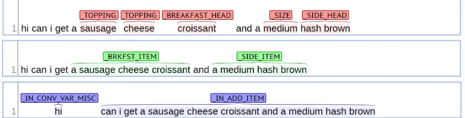
Figure2 is an example of an utterance labeled with the three levels of our annotation scheme. In this example, there are two items, a sausage cheese croissant and a medium hash brown, which can be decomposed into five entities, sausage, cheese, croissant, medium, and hash brown. Thus, it shows the compositional nature of of food item specification in this annotation scheme.

Figure 2: Annotation on the Three Levels

entity/item/intent and it is possible, even likely, that there is more than one span in each utter-ance. For example, in Figure2, the example utter-ance contains two intents, IN CONV MISC and

IN ADD ITEM.

3.2 Synthetic Data Set

The synthetic data generator consists of a context free grammar that generates not only customer ut-terances but also the entities, items, and intents that go with each utterance. The grammar con-sists of rules each having nonzero positive inte-ger weights. Rules to generate entities correspond to menu items and ways to specify variations of menu items (e.g. small versus large). Customer utterances are generated by randomly selecting rules from the grammar, simulating a context free derivation.

There are 170 rules to generate intent se-quences, 1275 rules to generate items, and 450 rules to generate entities. For our experiments, the data generator was run so that 55,000 synthetic ut-terances were generated.

3.3 Sequence Labeling as a Classification Task

Sequence labeling can be treated as a set of in-dependent classification tasks, one per member of the sequence. We acknowledge that the accuracy is generally improved by making the optimal la-bel for a given element dependent on the choices of nearby elements, using special algorithms to choose the globally best set of labels for the en-tire sequence at once (Erdogan,2010).

However, we would like to present our k-NN classification appproach. With the help of post-processing, our approach yields better results compared to classic MEMMs, CRFs or neural net-works.

In our approach, each word in the utterance is labeled independently. Post-processing is per-formed for each utterance after all the words are labeled. The post-processing step contains two ac-tions:

1. If an N-word span does not begin with a be-ginning (B-) tag, correct it to be a bebe-ginning tag.

2. In an N-word span, if several enti-ties/items/intents are identified, per-form a majority vote to unify the enti-ties/items/intents.

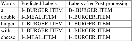
Table 1is a comparison between the predicted labels and the labels after post-processing. For ex-ample, the predicted label for a certain span may look like the second column in Table1. There are two obvious prediction mistakes we can systemat-ically correct without introducing new ones. The first IOB tag can be corrected from ”I-” to ”B-” since it is the beginning of the chunk. Since there is a two-to-three split in the item labels, we can also unify the labels by taking a majority vote to make them all ” BURGER ITEM”.

We will show in Section4that post-processing will improve upon the classification results.

3.4 Experiment Setup

Our series of experiment contains four subsets of experiments. The results are presented in Section 4and discussed in Section5.

Words Predicted Labels Labels after Post-processing a I- BURGER ITEM B- BURGER ITEM

double I- MEAL ITEM I- BURGER ITEM burger I- BURGER ITEM I- BURGER ITEM with I- BURGER ITEM I- BURGER ITEM cheese I- MEAL ITEM I- BURGER ITEM

Table 1: Predicted and Post-processed Labels

We tested on both human transcribed and ASR data.

In the third set of experiments, we investi-gate how semi-supervised training can help with the classification task. We obtained additional unannotated but human transcribed data only one eighth the size of our synthesized data. We used the annotated human transcribed data, which is identical to the training set in the second set, as our seeding data and performed prediction on our additional data set. We use the distance as a con-fidence measure, so we could set multiple thresh-olds and add the prediction as additional training data to our training set. The thresholds were set at the first, second and third quartile. We also ex-perimented with only using the predictions of the additional data as our training set. In this exper-iment setting, all the predictions that have a dis-tance of zero, which is a confidence of 100%, are also removed to increase the diversity of the train-ing set as this kind of predictions are simply exact matches to the seeding training set.

In the fourth set of experiments, we moved back to using only the annotated human transcribed training data. However, with the help of ASR im-provement, we tested on a more accurate test set. We performed post-processing in this set of exper-iments as well.

In experiments comparing TiMBL with the use of other classifiers, we specifically compare against MEMM (McCallum et al., 2000) and BiLSTM-CRF with ELMO embeddings (Peters et al., 2018). For the BiLSTM-CRF we use the Baseline open source software package (Pressel et al.,2018).

All experiments include parameter optimization in reported results.

3.5 Features

Most machine learning models prefer homoge-neous data. We usually use data of the same type in one feature matrix. For example, in

bag-of-words (BOW) approach towards text classifi-cation, we fill in every cell of the matrix with a Boolean value (present/absent) of a certain word or character n-gram. Another example would be, for image classification, we pass the raw pixel value to a deep neural network. Such vector rep-resentations of words and sentences are also com-mon acom-mong recent works in natural language pro-cessing. Word2vec, GloVe and ELMO word em-beddings are especially popular in recent years. These kind of vector representations are generally used with a neural network classifier too (Peters et al.,2018).

To the best of our knowledge, no previous re-search has investigated using both symbolic fea-tures and vector representations in a single k-NN classifier for sequence labeling. We present this new feature vector, the concatenation of two types of features. In our approach, we use three kinds of features, two of them being symbolic and one of them being a vector representation. Our features are:

1. Windowed left and right 5 word unigrams

2. Windowed left and right 5 part-of-speech (POS) tag unigrams

3. 25-dimensional GloVe word embedding vec-tors

Windowed word unigrams refer to a sequence of words like this: For a given word w, the win-dowed word unigrams are w-4, w-3, w-2, w-1, w, w+1, w+2, w+3, and w+4. Here we are using the window size of 5. This parameter was optimized in our pilot study.

GloVe vectors are designed to capture a word as its relation to its co-occurrent words in the global corpus (Pennington et al., 2014). Since k-NN classifiers are better at handling fewer number of symbolic and abstract features, we chose the 25-dimensional word vector. This is also under the consideration that k-NN classifier will weigh fea-tures and we would like to maintain enough weight for our symbolic features. We also did pilot study to determine the best dimensionality and the re-sult is consistant with our observation. All hyper-parameters of the classifier are optimized using leave-one-out method on the training set.

4 Results

In this section we present our evaluation results. All the numbers are calculated using the labeled bracketed score. For example, if a n-word span is labeled as N, the predictions need to match both the left and the right boundaries and the label N unanimously to be counted as one correct predic-tion. If the predictions have the wrong word span or at least one wrong label, the entire chunk is con-sidered incorrect.

4.1 Experiment Results

The results are shown in Table3.

In the Experiment I, using synthesized training data and human transcribed (HT in Table 3) test data produced the best result. Overall we achieved an F-score of 41.25.

In the Experiment II, the leave-one-out experi-ment performed on human transcribed data is used to show the upper bound of the task (italicized in Table3). This is the ideal situation in which we do not introduce errors from automatic speech recog-nition. The distribution of training set and the test set is identical. In this best scenario, our classifier achieved an F-score of 61.33.

In the Experiment III, we have two different set-tings. One of them is to use both human tran-scribed data and additional self-training labeled data, the other is to only use human transcribed data as the seed while the training set itself is the sole self-training labeled data. The second setting is closer to real world scenario especially when we are dealing with situations like a cold start. In this set, human transcribed data plus additional self-training labeled data reached an F-score of 48.30, outperforming only the additional data by slightly over four points.

In the Experiment IV, we show that with the ac-curacy improvement from ASR, our F-score is im-proving as well. By performing post-processing, which is a process that is designed strictly to cor-rect errors without compromising the performance in the long run, we manage to achieve close to up-per bound up-performance with an F-score of 60.71.

4.2 Multilevel Results

The best performance for all levels is achieved when we have improved ASR output and perform post-processing to correct the errors caused by the nature of classification.

However, the results in the third set of experi-ment show some interesting trends. When training with human transcribed data, the best performance is achieved with the least additional data. Mean-while, when training without human transcribed data, the best performance is achieved with the most additional data. Even this cannot produce comparable results to the experiments with human transcribed data.

4.3 Results of Using Other Classifiers

Overall we achieve 60.71 F measure on ASR input using TiMBL. In comparison, as shown in Figure 4, two previous systems, MEMM and BiLSTM-CRF, achieved 48.26 and 47.75 respec-tively. When hand transcribed text is input, BiLSTM-CRF performs the best, 69.15 F, fol-lowed by MEMM and TiMBL at 67.37 F and 61.3 F, respectively.

4.4 Running Times

The running times for different classifiers are shown in Figure5. It can be seen that while the BiLSTM-CRF may be a better classifier than the MEMM in terms of accuracy, there is a trade-off in terms of running time. It may be noted, how-ever, that degradation of performance at test time for BiLSTM-CRF is not as severe as the perfor-mace drop during training.

5 Discussion

In this section we discuss our findings from our experiments.

5.1 Experiment I

Training Set Size Test Set Size Experiment I Synthesized 464,675 Human Transcription (HT) 3,610 Synthesized 464,675 Automatic Speech Recognition 3,336 Experiment II Human Transcription 3,610 HT leave-one-out 3,610 Human Transcription 3,610 Automatic Speech Recognition 3,336 Experiment III (1) HT + 25% Additional 17,134 Automatic Speech Recognition 3,336 HT + 50% Additional 30,657 Automatic Speech Recognition 3,336 HT + 75% Additional 44,180 Automatic Speech Recognition 3,336 HT + 100% Additional 57,703 Automatic Speech Recognition 3,336 Experiment III (2) Seeded 25% 14,617 Automatic Speech Recognition 3,336 Seeded 50% 29,223 Automatic Speech Recognition 3,336 Seeded 75% 43,849 Automatic Speech Recognition 3,336 Seeded 100% 58,465 Automatic Speech Recognition 3,336 Experiment IV Human Transcription 3,715 Automatic Speech Recognition 3,509 Human Transcription 3,715 ASR + Post-processing 3,509

Table 2: Experiment Setup

Training / Test Entity Item Intent All Experiment I Synthesized / HT 65.59 23.24 33.60 41.25 Synthesized / ASR 51.14 12.81 19.39 27.51 Experiment II HT leave-one-out 80.11 43.25 53.30 61.33 HT / ASR 66.53 37.70 38.07 48.76 Experiment III (1) HT + 25% / ASR 66.26 37.06 37.65 48.30 HT + 50% / ASR 65.60 36.55 37.08 47.75 HT + 75% / ASR 66.31 35.31 36.71 47.44 HT + 100% / ASR 66.26 35.38 37.18 47.68 Experiment III (2) Seeded 25% / ASR 48.53 20.71 32.07 35.59 Seeded 50% / ASR 60.04 27.10 33.39 41.89 Seeded 75% / ASR 62.95 30.52 33.87 43.91 Seeded 100% / ASR 64.29 30.70 33.61 44.28 Experiment IV HT / Better ASR 75.39 51.37 45.03 57.87 HT / ASR + Post-processing 75.46 52.84 49.66 60.71

Table 3: Experiment Results (F-score)

later. Compared to testing on human transcribed data, testing on ASR data performed much worse with a decrease of almost fourteen points in terms of F-score. Human transcribed data tend to be more grammatical and relevant. As we can see in our first example, ASR data has a lot more noise. The word sequences occurred in the sentence are also less common. Words that sound similar can be mistaken from each other. However, this poses some difficulty on the POS tagger when it tries to tag the words based on the left and right context. We believe this is one of the reasons we saw a big performance difference here.

5.2 Experiment II

The leave-one-out experiment with the human transcribed data serves as the upper bound, the ideal situation where the distribution is identical and no error is introduced externally. However, it is unlikely to achieve such result in real life sce-nario since user input is noisy and external errors will be introduced along the pipeline inevitably.

Model Training / Test Entity Item Intent All MEMM HT 10-fold CV 73.22 55.22 67.21 67.37 HT / Better ASR 60.87 32.97 42.92 48.26 BiLSTM-CRF HT 10-fold CV 77.16 59.12 66.54 69.15 HT / Better ASR 62.97 33.90 39.45 47.57

Table 4: Comparable Results (F-score)

Model Training Time Test Time MEMM 18.00 seconds 10.00 seconds BiLSTM-CRF 1 hour 27.80 seconds TiMBL 0.19 second 3.05 seconds

Table 5: Times taken to train and test different classi-fiers over one fold of the test corpus.

this shows that with very little training data we can still achieve rather decent results. The closer the distribution of both data sets have, the more likely we can achieve higher accuracy. Having just a lit-tle bit of human transcribed and annotated data is a reasonable cost for higher quality prediction.

5.3 Experiment III

This is a set of experiment that is rather a rein-forcement of the second experiment. Though the F-score dropped minimally due to the added noise from the additional data, it is still obvious that by using real world data we are improving the accu-racy.

The second half of this set of experiment pro-vides a potential alternative to our approach. As much as the result is not as good as the first half of this experiment or the second set of experiments, it is still even more accurate than the first set of experiments. With better ASR quality we believe semi-supervised self-training can and should help.

5.4 Experiment IV

This is our best and state-of-the-art result of this task. With the help from ASR quality improve-ment, the classifier receives a significant boost in performance from an F-score of 48.76 to 57.87.

It is especially worth noticing that by post-processing we achieve 3 points even more. Post-processing is strictly used to correct the inconsis-tency in the predictions as each individual decision is made independent of each other. It will not hurt the performance in the long run.

5.5 Using Other Classifiers

It is interesting to note that the BiLSTM-CRF performs the worst on ASR input, perhaps be-cause the ELMO embeddings that are used by the BiLSTM-CRF are sensitive to the context of the whole utterance, and this context can differ quite a lot between the training utterances which are hand transcribed and the test utterances which are pro-vided by ASR.

6 Conclusion

In this paper we present a new method to perform multi-level sequence labeling. We show that this method actually outperforms other state-of-the-art methods for this task, showing k-NN is competi-tive with other methods in the not infrequent situ-ation where only a small amount of training data is available.

We achieved labeled bracketed F-scores of 75.46, 52.84 and 49.66 for the three levels of se-quence labeling. Overall we achieved 60.71 at all levels.

7 Future Work

We believe that the pipeline should be fully tomated for production purposes. We could au-tomate how the rules are obtained, or extend the rules to correct more mistakes.

As a future research direction for conversational AI, we think that to train and test a k-NN model for predicting which dialog move to take will be beneficial as well.

References

Steven Bird and Edward Loper. 2004. Nltk: the nat-ural language toolkit. In Proceedings of the ACL 2004 on Interactive poster and demonstration ses-sions, page 31. Association for Computational Lin-guistics.

nlu for customer ordering dialogs. InProceedings of IEEE SLT 2018 Workshop on Spoken Language Technology, Athens, Greece.

Walter Daelemans, Jakub Zavrel, Kurt Van Der Sloot, and Antal Van den Bosch. Timbl: Tilburg memory-based learner.

Layla El Asri, Hannes Schulz, Shikhar Sharma, Jeremie Zumer, Justin Harris, Emery Fine, Rahul Mehrotra, and Kaheer Suleman. 2017. Frames: A corpus for adding memory to goal-oriented dialogue systems. InProceedings of the SIGDIAL 2017 Con-ference, pages 207–219, Saarbr¨ucken, Germany.

Hakan Erdogan. 2010. Sequence labeling: Generative and discriminative approaches. iCMLA.

Dilek Hakkani-T¨ur, Gokhan T¨ur, Asli Celikyilmaz, Yun-Nung Vivian Chen, Jianfeng Gao, Li Dung, and Ye yi Wang. 2016. Multi-domain joint semantic frame parsing using bi-directional rnn-lstm. In Pro-ceedings of The 17th Annual Meeting of the Interna-tional Speech Communication Association (INTER-SPEECH 2016).

Charles T Hemphill, John J Godfrey, and George R Doddington. 1990. The ATIS spoken language sys-tems pilot corpus. InSpeech and Natural Language: Workshop Proceedings, Hidden Valley, Pennsylva-nia.

Mitchell P Marcus, Mary Ann Marcinkiewicz, and Beatrice Santorini. 1993. Building a large annotated corpus of english: The penn treebank. Computa-tional linguistics, 19(2):313–330.

Andrew McCallum, Dayne Freitag, and Fernando CN Pereira. 2000. Maximum entropy markov models for information extraction and segmentation. In

Icml, volume 17, pages 591–598.

Jeffrey Pennington, Richard Socher, and Christopher Manning. 2014. Glove: Global vectors for word representation. InProceedings of the 2014 confer-ence on empirical methods in natural language pro-cessing (EMNLP), pages 1532–1543.

Matthew E Peters, Mark Neumann, Mohit Iyyer, Matt Gardner, Christopher Clark, Kenton Lee, and Luke Zettlemoyer. 2018. Deep contextualized word rep-resentations. arXiv preprint arXiv:1802.05365.

Daniel Pressel, Sagnik Ray Choudhury, Brian Lester, Yanjie Zhao, and Matt Barta. 2018. Baseline: A library for rapid modeling, experimentation and development of deep learning algorithms targeting NLP. In Proceedings of Workshop for NLP Open Source Software, pages 34–40.

Marilyn A. Walker, Owen Rambow, and Monica Ro-gati. 2001. SPoT: A trainable sentence planner. In Proceedings of the second meeting of the North American Chapter of the Association for Computa-tional Linguistics on Language technologies.