Proceedings of NAACL-HLT 2019, pages 3784–3794 3784
Continuous Learning for Large-scale Personalized Domain Classification
Han Li1,Jihwan Lee2,Sidharth Mudgal2,Ruhi Sarikaya2, andYoung-Bum Kim2
1University of Wisconsin, Madison
2Amazon Alexa AI
{jihwl, sidmsk, rsarikay, youngbum}@amazon.edu
Abstract
Domain classification is the task of mapping spoken language utterances to one of the natu-ral language understanding domains in intelli-gent personal digital assistants (IPDAs). This is a major component in mainstream IPDAs in industry. Apart from official domains, thou-sands of third-party domains are also created by external developers to enhance the capa-bility of IPDAs. As more domains are de-veloped rapidly, the question of how to con-tinuously accommodate the new domains still remains challenging. Moreover, existing con-tinual learning approaches do not address the problem of incorporating personalized infor-mation dynamically for better domain classi-fication. In this paper, we propose CONDA, a neural network based approach for domain classification that supports incremental learn-ing of new classes. Empirical evaluation shows that CONDA achieves high accuracy and outperforms baselines by a large margin on both incrementally added new domains and existing domains.
1 Introduction
Domain classification is the task of mapping spo-ken language utterances to one of the natural lan-guage understanding (NLU) domains in intelligent personal digital assistants (IPDAs), such as Ama-zon Alexa, Google Assistant, and Microsoft
Cor-tana, etc. (Sarikaya,2017). Here a domain is
de-fined in terms of a specific application or function-ality such as weather, calendar or music, which narrows down the scope of NLU. For example,
given an utterance “Ask Uber to get me a ride”
from a user, the appropriate domain would be one that invokes the “Uber” app.
Traditionally IPDAs have only supported dozens of well-separated domains, where each is defined in terms of a specific application or
func-tionality such as calendar and weather (Sarikaya
et al., 2016; Tur and De Mori, 2011; El-Kahky et al.,2014). In order to increase the domain cov-erage and extend the capabilities of the IPDAs, mainstream IPDAs released tools to allow
third-party developers to build new domains.
Ama-zons Alexa Skills Kit, Googles Actions and Mi-crosofts Cortana Skills Kit are examples of such tools. To handle the influx of new domains,
large-scale domain classification methods like SHORT
-LISTER (Kim et al., 2018b) have been proposed and have achieved good performance.
As more new domains are developed rapidly, one of the major challenges in large-scale domain classification is how to quickly accommodate the new domains without losing the learned predic-tion power on the known ones. A straightforward solution is to simply retraining the whole model whenever new domains are available. However, this is not desirable since retraining is often time consuming. Another approach is to utilize con-tinual learning where we dynamically evolve the model whenever a new domain is available. There is extensive work on the topic of continual learn-ing, however there is very little on incrementally adding new domains to a domain classification system.
To mitigate this gap, in this paper we propose
the CONDA solution for continuous domain
adap-tation. Given a new domain, we keep all learned parameters, but only add and update new parame-ters for the new domain. This enables much faster model updates and faster deployment of new fea-tures to customers. To preserve the learned knowl-edge on existing domains to avoid the notorious
catastrophic forgetting problem (Kemker et al.,
2018), we propose cosine normalization for output
with the new domain data for continuous domain adaptation. This is shown to further alleviate the
overfitting on the new domain data. Empirical
evaluation on real data with 900 domains for initial training and 100 for continuous adaptation shows
that CONDA out performs the baselines by a large
margin, achieving 95.6% prediction accuracy on average for the 100 new domains and 88.2% accu-racy for all seen domains after 100 new domains have been accommodated (only 3.6% lower than the upperbound by retraining the model using all domain data). To summarize, we make the follow-ing contributions in this paper:
• We introduce the problem of continuous
do-main adaptation for large-scale personalized domain classification.
• We describe CONDA, a new solution for
continuous domain adaptation with Cosine normalization, domain embedding regular-ization and negative exemplar sampling tech-niques. Our solution advances the research in continuous domain adaptation.
• We conduct extensive experiments showing
that CONDA achieves good accuracy on both
new and existing domains, and outperforms the baselines by a large margin.
2 Background and Problem Definition
2.1 Domain Classification
Domain classification is the task of mapping spo-ken language utterances to one of the NLU do-mains in IPDAs. A straightforward solution to tackle this problem is to ask users to explicitly mention the domain name with a specific
invoca-tion pattern. For example, for the utterance “Ask
Uber to get me a ride”, the invocation pattern is “Ask {domain} to {perform action}”. While it makes things much simpler for the domain clas-sifier, this significantly limits natural interaction with IPDAs as users need to remember the do-main names as well as the invocation pattern. To
address this limitation, name-free domain
classi-fication methods were developed for more user
friendly interactions, and have been getting more attention recently. We specifically focus on the name-free scenario in this paper.
2.2 The Shortlister System
To our knowledge, the state-of-the-art for
name-free domain classification is SHORTLISTER (Kim
et al., 2018b), which leverages personalized user provided information for better classification
per-formance. Specifically, it contains three main
modules.
The first module is the LSTM-based encoder to map an utterance to a dimension-fixed vector representation. Given an utterance, each word is first represented as dense vectors using word
em-beddings, then a bidirectional LSTM (Graves and
Schmidhuber,2005) is be used to encode the full utterance.
The second module is the personalized domain summarization module. For each utterance from an IPDA user, a list of domains have been enabled by the user. These enabled domains can be viewed as user-specific personalized information. It has been shown that the domain classification accu-racy can be significantly improved by leveraging
information about enabled domains (Kim et al.,
2018b). To represent the domain enablement in-formation, first each enabled domain is mapped to a fixed-dimensional embedding, then a summa-rization vector is generated by taking an attention
weighted sum (Luong et al., 2015) over the
en-abled domain embeddings.
Once the utterance representation and the en-abled domain summarization are calculated, we concatenate the two vectors as the final represen-tation. Then the third module, a feed-forward net-work, is used to predict the confidence score with a sigmoid function for each domain.
2.3 Continuous Domain Adaptation
As more new domains are developed, a major challenges in large-scale domain classification is quickly accommodating the new domains into the live production domain classification model with-out having to perform a full retrain. We refer to
this problem as Continuous Domain Adaptation
(CDA). In this paper, we specifically focus on the case of purely online learning where new domains where added one by one, since in practice we want to quickly integrate a new domain into the system as soon as it becomes available. We formally de-fine the problem below.
Definition 1 (Online continuous domain
adapta-tion) Given a collection of k domains Sk =
{s1, s2, . . . , sk}, suppose we have a dataset Dk
the enabled domainsE ⊆ Sk. DenoteP(Sk) as the powerset ofSk, a modelMk :U × P(Sk) →
Skhas been trained onDkfor domain classifica-tion with the accuracy Mk(Dk). At some point, a new domain sk+1 is available with the
corre-sponding dataset Dk+1 = {(u, sk+1, E) | E ⊆
Sk+1}withSk+1 = Sk∪ {sk+1}. Taking
advan-tage ofDk+1, the continuous adaptation forsk+1
is to updateMktoMk+1:U× P(Sk+1)→Sk+1
so that the model can make predictions forsk+1,
with the goal of maximizing Mk+1(Dk+1) and
minimizingMk(Dk)−Mk+1(Dk).
3 The CoNDA Solution
We introduce CONDA (Continuous Neural
DomainAdaptation), a variation of SHORTLISTER
that is capable of handling online CDA decribed
in Definition1. Similar to SHORTLISTER, it has
three main modules.
The first module is the LSTM-based utterance encoder which shares the same architecture as the
one used in SHORTLISTER, that maps an input
ut-terance into a dense vector. After the training on
the initialk-domain dataDk, we freeze all
param-eters (i.e., the word embedding lookup and the bi-LSTM parameters) of this module from changing for the subsequent online domain adaptation tasks.
Usually the value ofk is large enough (hundreds
or even thousands in real-world, at least 100 in our experiments), thus it is safe to assume that the pa-rameters have been tuned sufficiently well to en-code utterances from all existing and future do-mains. In this work we treat new words in the new domains as unknown and leave the problem of vocabulary expansion as future work.
The second module is the personalized domain summarization module which will map the en-abled domains of an input utterance to a dense vector representation. It is also similar to the one in SHORTLISTER, except we will evolve the mod-ule as we are adding new domains. Specifically,
given datasetDkonkdomains for initial training,
a domain embedding table Tk ∈ Rk×ds will be
learned wheredsis the size of the domain
embed-dings. When a new domainsk+1 is available, we
expandTktoTk+1 ∈ R(k+1)×ds by: (1) freezing
the learned embeddings for all known domains;
(2) adding a new row tk+1 ∈ Rds to Tk as the
domain embedding forsk+1and updating the new
parameters tk+1 using all available training data
at hand (i.e., the dataset Dk+1 and the negative
samples which will be discussed later in this sec-tion). We repeat this procedure whenever a new
domain is available. To avoid over-fitting ontk+1,
we introduce a new regularization term into the loss function. We describe the details in Section
3.2.
The third module is a two-layer feed-forward
network as the classifier. The first layer f(1) :
Rdu+ds →Rdh maps the concatenation of the
ut-terance embedding (in sizedu) and domain
sum-marization (in sizeds) into fix-sized hidden
repre-sentation (in sizedh) using a fully connected layer
followed by SELU activation (Klambauer et al.,
2017), which is identical to the one in SHORTLIS
-TER. Then the prediction layerf(2) :Rdh → Rk
maps the hidden representation to the final domain
prediction scores. Unlike SHORTLISTER where
the final prediction score is the dot product of the weight vector and the hidden representation, we choose to use the cosine score of the two,
re-ferred to ascosine normalization. To support
on-line CDA when a new domain is available, we ap-ply a similar approach to the domain embedding expansion described above to expand the
predic-tion layer. Specifically, denote Wk(2) ∈ Rk×dh
be the weights for the prediction layer that has
been trained on the initialkdomains. To adapt the
new domain dk+1, we expand Wk(2) to W
(2)
k+1 ∈
R(k+1)×dh by first freezing all learned
parame-ters and adding a new row of learnable parameparame-ters
wk+1∈RdhtoW
(2)
k .
As each time we only add one new domain, all training utterances during the update will have the same label. Thus, it’s easy to overfit the new data such that catastrophic forgetting occurs. Inspired by (Rebuffi et al., 2017), we also propose a neg-ative sampling procedure to leverage (limited) in-formation on the known domains to alleviate the catastrophic forgetting problem. For the rest of the section, we will first talk about cosine normaliza-tion, and then domain embedding regularizanormaliza-tion, and finally negative sampling.
3.1 Cosine Normalization
As mentioned above, we use the cosine similarity of the weights and the hidden representation vec-tor instead of the linear dot product in the
predic-tion layer. Formally, letfk(2) :Rdh →[−1,1]kbe
the prediction layer forkdomains with parameters
Wk(2) ∈ Rk×dh. Given an input hidden
s1= “Weather”
sk+1= “Uber”
h
s1= “Weather”
sk+1= “Uber” h
θ2 θ1
[image:4.595.73.291.63.139.2](a) (b)
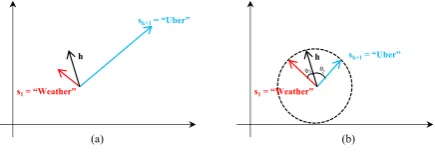
Figure 1: Cosine Example.
domain under cosine normalization is:
fk,i(2)(h) = cosh, Wk,i(2)= h·W
(2)
k,i
khk
W
(2)
k,i
(1)
To understand why cosine is better in the case of online CDA, let’s first see the problem with the dot-product method. Suppose we are
accommo-datingsk+1 with dataset Dk+1, because we train
the new parameters wk+1 only on Dk+1 where
all utterances have the same domain sk+1, the
model can easily get good training performance on
Mk+1(Dk+1)by simply maximizing the values in
wk+1such that the dot product of the hidden
repre-sentation withwk+1is larger than the dot product
with any other wi,1 ≤ i ≤ k. Effectively this
leads to the model predicting domainsk+1for any
given utterance. Using cosine normalization
in-stead as described in Eq. 1removes the incentive
to maximize the vector length ofwk+1.
Example 1 SupposeMkhas been initially trained
onDk, and domains1=“Weather”. Given an
ut-terance u = “What’s the weather today?”, Mk
correctly classifiesuintos1. Now a new domain
sk+1=“Uber” is coming and we evolve Mk to
Mk+1. As the norm of the weightswk+1could be
much larger thanw1 in the prediction layer, even
if the hidden representationhofuis closer tos1in
direction,Mk+1will classifieruintosk+1as it has
a higher score, shown in Figure1.a. However if we measure the cosine similarity,Mk+1 will
clas-sifyucorrectly because we now care more about the directions of the vectors, and the angleθ1
be-tween h and s1 is smaller (representing higher
similarity) than the angleθ2 betweenhandsk+1,
as shown in Figure1.b.
As we use the cosine normalization, all pre-diction scores are mapped into the range [-1, 1]. Therefore it’s not proper to use log-Sigmoid loss
function as in SHORTLISTER. So accompanying
with the cosine normalization, the following hinge
loss function has been used instead:
(2)
Lhinge=
n
X
i=1
yimax{∆pos−oi,0}
+
n
X
i=1
(1−yi) max{oi−∆neg,0}
wherenis the number of all domains,oiis the
pre-dicted score for each domain,yis an-dimensional
one-hot vector with 1 in the ground-truth label and
0 otherwise. ∆posand∆neg are the hinge
thresh-olds for the true and false label predictions respec-tively. The reason we use hinge loss here is that it can be viewed as another way to alleviate the over-fitting on new data, as the restrictions are less by only requiring the prediction for the ground-truth
to be above∆posand false domain predictions
be-low ∆neg. Our experiments show that this helps
the model get better performance on the seen do-mains.
3.2 Domain Embedding Regularization
In this section, we introduce the regularizations on the domain embeddings used in the personalized domain summarization module. Recall that given
an utterance u withhu as the hidden
representa-tion from the encoder and its enabled domainsE,
personalized domain summarization module first
compares u with each si ∈ E (by calculating
the dot product ofhu and the domain embedding
ti of si) to get a score ai, then gets the weight
ci = exp (ai)/Pajexp (aj)for domainsi, and
fi-nally computes the personalized domain summary
asP
ei∈Eci·ti. We observed that after training on
the initial datasetDk, the domain embedding
vec-tors tend to roughly cluster around a certain (ran-dom) direction in the vector space. Thus, when
we add a new domain embeddingsk+1to this
per-sonalization module, the model tends to learn to move this vector to a different part of the vector space such that its easier to distinguish the new domain from all other domains. Moreover, it also
increases the`2 norm of the new domain
embed-dingtk+1to win over all other domains.
Example 2 Suppose a similar scenario to
Exam-ple1where we haves1= “Weather” inSkand a
new domainsk+1 = “Uber”. As most utterances
inDk+1havesk+1as an enabled domain, it’s easy
for the model to learn to enlarge the norm of the
new domain embedding tk+1 as well as make it
can dominate the domain summarization. Then
coordinating with the new weights wk+1 in the
prediction layerfk(2)+1, the network can easily pre-dict high scores sk+1 and fit the dataset Dk+1.
However, when we have utterances belonging to
s1 with sk+1 as an enabled domain, sk+1 may
still dominate the summarization which makes the prediction layer tends to cast those utterances to sk+1. We don’t observe this on the initial training
on Dk becausesk+1 was not visible at that time,
thus cannot be used as an enabled domain. And it’s even worse ifs1is similar tosk+1in concept.
For example ifs1 = “Lyft”, in this case the
utter-ances of the two domains are also similar, making the dot product oftk+1and the hidden
representa-tions of thes1’s utterances even larger.
To alleviate this problem, we add a new domain embedding regularization term in the loss func-tion to constrain the new domain embedding vec-tor length and force it to direct to a similar area where the known domains are heading towards, so that the new domain will not dominate the domain summarization. Specifically,
(3)
Lder =
k
X
i=1
λimax{∆der−cos(tk+1, ti),0}
+λnorm
2 ktk+1k
2
We call the first part of Eq. 3 on the right
hand side as thedomain similarity losswhere we
ask the new domain embedding tk+1 to be
simi-lar to known domainti’s controlled by a
Cosine-based hinge loss. As we may not need tk+1 to
be similar to all seen domains, a coefficient λi is
used to weight the importance each similarity loss
term. In this paper we encouragetk+1 to be more
similar to the ones sharing similar concepts (e.g. “Uber” and “Lyft”). We assume all training data are available to us, and measure the similarity of two domains by comparing their average of utter-ance hidden representations.
Specifically, denote ϕ : U → Rdu as the
LSTM-encoder that will map an utterance to its
hidden representation with dimension du. For
each domainsi ∈Sk+1, we first calculate the
av-erage utterance representation onDi
e
hi =
X
(u,si,e)∈Di
ϕ(u)
|Di| (4)
Then we set λi = λdslmax{cos(ehi,ehk+1),0}
withλdslas a scaling factor.
Combining Eq. 2and3, the final loss function
for optimization is:Ltotal=Lhinge+Lder
3.3 Sampling Negative Exemplars
So far we developed our method by training only
on the new dataDk+1, and use regularizations to
prevent overfitting. However, in many real
appli-cations all of the training data, not onlyDk+1, is
actually available, but it’s not affordable to retrain
the full model using all data. Inspired by (Rebuffi
et al.,2017), we can select a set of exemplars from the previously trained data to further improve con-tinual adaptation.
Suppose we are handling the new domainsk+1
withDk+1, and all data trained previously isDk
on k domains Sk. For each known si ∈ Sk,
we pick N utterances from Di as the exemplars
for si. Denote Pi be the exemplar set forsi and
P = Sk
i=1Pi be the total exemplar set. To
gen-erate eachPi, we pick the top-N utterances that
are closest to the average of the utterance hidden
representation. Specifically, following Eq. 4, we
first get the average representation ehi, then Pi is
defined as follow:
Pi =Pi⊆Di,|Pi|=N X
(u,si,e)∈Pi
cosϕ(u),ehi
(5)
If multiple candidates satisfying Eq. 5forPi, we
randomly pick one asPito break the tie. Once the
domain adaptation forsk+1 is done, we similarly
generate Pk+1 and merge it toP. We repeat this
procedure for negative sampling whenever a new domain is coming later.
As we add more new domains, the exemplar set
P also grows. For some new domain Dk+1, we
may have |P| |Dk+1|. In this case, the
pre-diction accuracy on the new domain data could be very low as the model will tend to not making
mis-takes onP rather than fitting Dk+1. To alleviate
this problem, when|P|>|Dk+1|, we select a
sub-set P0 ⊆ P with |P0|= |Dk+1|, and P0 will be
used as the final exemplar set to train together with
Dk+1. To generateP0, we just randomly sample a
subset fromP, since it was observed to be
effec-tive in our experiments.
4 Empirical Evaluation
4.1 Experiment Setup
Dataset: We use a dataset defined on 1000
80 90 100
10 20 30 40 50 60 70 80 90 100
Accuracy on each new domain
-5 10 25 40 55 70 85 100
1 5 9 13 17 21 25 29 33 37 41 45 49 53 57 61 65 69 73 77 81 85 89 93 97
Accumulated accuracy on previously trained new domains
Ac
cu
ra
cy
Number of newdomains Number of new domains
-5 5 15 25 35 45 55 65 75 85 95
1 5 9 13 17 21 25 29 33 37 41 45 49 53 57 61 65 69 73 77 81 85 89 93 97
Accumulated accuracy on all previously known domains
linear-full-update linear cos cos+ns cos+der cos+der+ns upperbound
Number of new domains
[image:6.595.82.523.60.152.2](a) (b) (c)
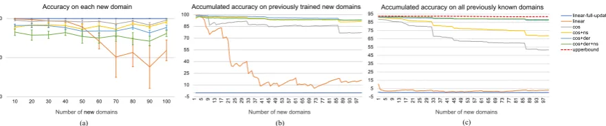
Figure 2: Overall evaluation. (a) shows the accuracy for new domains. (b) shows the accumulated accuracy for previous new domains that have been adapted to the model so far. (c) shows the accumulated accuracy for all known domains including the ones used for initial training and all previously adapted new domains.
80 82 84 86 88 90 92 94 96 98 100
1 5 9 13 17 21 25 29 33 37 41 45 49 53 57 61 65 69 73 77 81 85 89 93 97
Performance of 100 initial training domains
80 82 84 86 88 90 92 94 96 98 100
1 5 9 13 17 21 25 29 33 37 41 45 49 53 57 61 65 69 73 77 81 85 89 93 97
Performance of 500 initial training domains
Ac
cu
ra
cy
Number of new domains Number of new domains
80 82 84 86 88 90 92 94 96 98 100
1 5 9 13 17 21 25 29 33 37 41 45 49 53 57 61 65 69 73 77 81 85 89 93 97
Performance of 900 initial training domains
new domain accumu. new domains accumu. all upperbound
Number of new domains
[image:6.595.74.527.205.298.2](a) (b) (c)
Figure 3: The model performance on different number of initial training domains. The red dashed line shows the upperbound of the accumulated accuracy, which is generated by retraining the model on all domains seen so far.
part contains 900 domains where we use it for the initial training of the model. It has 2.06M utter-ances, and we split into training, development and test sets with ratio of 8:1:1. We refer to this dataset as “InitTrain”. The second part consists of 100 domains and is used for the online domain adap-tation. It has 478K utterances and we split into training, development and test sets with the same 8:1:1 ratio. We refer to this dataset as “IncTrain”.
Training Setup: We implement the model in
PyTorch (Paszke et al., 2017). All of the
ex-periments are conducted on an Amazon AWS
p3.16xlarge1cluster with 8 Tesla V100 GPUs. For
initial training, we train the model for 20 epochs with learning rate 0.001, batch size 512. For the continuous domain adaptation, we add the new do-mains in a random order. Each domain data will be trained independently one-by-one for 10 epochs, with learning rate 0.01 and batch size 128. For both training procedures, we use Adam as the op-timizer. The development data is used to pick the best model in different epoch runs. We evaluate the classification accuracy on the test set.
4.2 Overall Performance
We first talk about the overall performance. In our experiments we select two baselines. The first one
linear-full-updatewhich simply extends
1https://aws.amazon.com/ec2/instance-types/p3/
SHORTLISTERby adding new parameters for new domains and conducting full model updating. The
secondlinearis similar to the first baseline
ex-cept that we freeze all trained parameters and only allow new parameter updating. Both the two
base-lines update the model with Dk+1 dataset only.
To show the effectiveness of each component of
CONDA, we choose four variations. The first one
is cos where we apply the Cosine
Normaliza-tion (CosNorm). The second one cos+der
ap-plies CosNorm with the domain embedding
reg-ularization. The third one cos+ns uses both
CosNorm and negative exemplars. And the last
onecos+der+nsis the combination of all three
techniques, which is our CONDA model. For
hyperparameters, we pick ∆pos = 0.5,∆neg =
0.3,∆der = 0.1, λdsl= 5, andλnorm = 0.4.
Figure 2 shows the accuracy for new
do-main adaptations. From the figure, here are the main observations. First, without any constraints,
linear-full-updatecan easily overfits the
new data to achieve 100% accuracy as shown in
Figure 2(a), but it causes catastrophic forgetting
such that the accuracy on seen domains is (almost)
0 as shown in Figure2(b) and (c). By freezing the
all trained parameters, the catastrophic forgetting
problem is a bit alleviated forlinear, but the
ac-curacy on the seen domains is still very low as we
add more new domains. Second, cos produces
lower accuracy on each new domain, showing the effectiveness of the Cosine normalization. Third, as we add more regularizations to the model, we get better accuracy on the seen domains (Figure
2 (b) and (c)), at the cost of sacrificing a bit on
the new domain accuracy (Figure 2 (a)). Also,
cos+der+ns(the CONDA model) achieves the
best performance, with an average of 95.6% ac-curacy for each new domain and 88.2% acac-curacy for all previously seen domains after we add 100 new ones, which is only 3.6% lower than the up-perbound (by retraining the model on the whole dataset). These demonstrate the superiority of our method.
4.3 Micro-benchmarks
Using Different Number of Initial Domains: We vary the number of domains for initial train-ing to see if it will have a big impact on the model performance. Specifically, we pick 100 and 500 domains from InitTrain, and use the same IncTrain
data for domain adaptation. Figure3compares the
model performance on these three different num-ber (i.e., 100, 500, 900) of initial training domains. From the figure we can see that the curves share a similar pattern regardless of the number of initial domains, showing that our model is stable to the number of domains used for initial training.
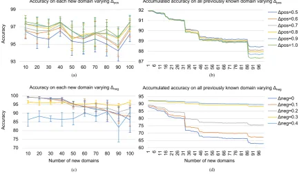
Varying the hinge loss thresholds: We vary the
classification hinge loss thresholds∆posand∆neg
to see how it will affect the performance.
Specif-ically, we fix∆neg = 0.3and vary∆pos from 0.5
to 1.0, and fix∆pos= 0.5and vary∆negfrom 0 to
0.4, respectively. For both of the them we use 0.1
as the step size. Figure4shows the model
perfor-mance. From the figures, we summarize the
fol-lowing observations. First, as we increase ∆pos,
on average the accuracy on each new domain gets
better (Figure 4(a)), but we loss performance on
all seen domains (Figure4(b)). This is in accord
with our intuition that a larger∆posputs more
con-straint on the new domain predictions such that it tends to overfit the new data and exacerbates catas-trophic forgetting on existing domains. Second, as
we increase∆neg, on average the accuracy on each
new domain gets worse (Figure 4(c)), but we get
better performance on existing domains. This is
because a larger ∆neg narrows down the
predic-tion “margin” between positive and negative
do-mains (similar to decreasing ∆pos), so that less
constraint has been put onto predictions to
allevi-ate overfitting on the new domain data.
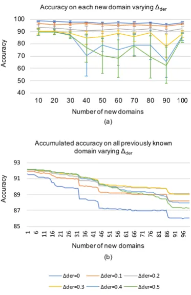
Varying the domain similarity loss threshold:
We vary the threshold∆der to see how it will
af-fect the model performance. Specifically, we vary
∆der from 0 to 0.5 with step size 0.1, and Figure
5shows the model performance. As we increase
∆der, the performance on the new domains gets
worse, and the drop is significant when ∆der is
large. On the other hand, the accumulated accu-racy on seen domains increases when we start to
increase∆der, and drops when∆der is too large.
This means we when we start to make the new domain embeddings to be similar to the existing ones, we alleviate the problem that the new do-main dominates the dodo-main summarization. Thus the accuracy on existing domains improves at the cost of sacrificing some accuracy on the new
do-mains. However, if we continue to increase∆der
to make it very similar to some of existing do-mains, the new domain will compete with some existing ones so that we loss accuracy on both new and existing domains.
Varying the weights for domain similarity loss: To see how the weighted domain similarity loss will affect the performance, we compare it against the plain version without the utterance
similar-ity weights. Specifically, we set eachλi = λdsl
having the same value. And our experiments
show that the plain version gets the average ac-curacy 94.1% on the new domains, which is 1.5% lower than the weighted version, and 88.7% ac-cumulated accuracy on all domains after adding 100 new domains, which is 0.5% higher than the weighted version. This means we can get a bit higher accumulated accuracy at the cost of sacri-ficing more new domain accuracy. In real appli-cations, the decision to whether use weighted do-main similarity loss should be made by trading off the importance of the new and existing domains.
Varying the number of used negative
exem-plars: As we mentioned before, we
down-sample the negative exemplar set P to reduce
93 95 97 99
10 20 30 40 50 60 70 80 90 100
Accuracy on each new domain varying Δpos
87 88 89 90 91 92
1 6 11 16 21 26 31 36 41 46 51 56 61 66 71 76 81 86 91 96 Accumulated accuracy on all previously known domain varying Δpos
Δpos=0.5 Δpos=0.6 Δpos=0.7 Δpos=0.8 Δpos=0.9 Δpos=1.0
70 75 80 85 90 95 100
10 20 30 40 50 60 70 80 90 100
Accuracy on each new domain varying Δneg
60 65 70 75 80 85 90 95
1 6 11 16 21 26 31 36 41 46 51 56 61 66 71 76 81 86 91 96 Accumulated accuracy on all previously known domain varying Δneg
Δneg=0 Δneg=0.1 Δneg=0.2 Δneg=0.3 Δneg=0.4
(a) (b)
(c) (d)
Ac
cu
ra
cy
Ac
cu
ra
cy
[image:8.595.82.516.64.317.2]Number of new domains Number of new domains
Figure 4: Model performance by varying the hinge loss thresholds. (a) and (b) shows accuracy on new domain and accumulated accuracy for all seen domains respectively by varying∆pos. Similarly, (c) and (d) shows the accuracy
performance by varying∆neg.
Prediction
Method 100 initial domains 500 initial domains 900 initial domains
Linear 95.2 93.9 93.4
Cosine 94.5 92.9 92.4
Table 1: Linear dot product versus Cosine normaliza-tion on initial training for different number of domains.
This means down-sampling effectively improve the model performance.
Effect of Cosine normalization in initial
train-ing: We have shown Cosine normalization with
hinge loss works better than linear dot product
with sigmoid loss (used in SHORTLISTER) for
CDA. Here we compare the two on the regular training setting where we train the model from scratch on a large dataset. Specifically, we com-pare the initial training performance on 100, 500, and 900 domains which are the same as we used
earlier. Table 1 shows the accuracy numbers.
From the table we see that Linear works better than Cosine by 0.7-1.0% across different number of domains. Though the difference is not large, this means Linear could be a better option than Cosine when we train the model from scratch.
Varying the order of the new domains: To see
if the incoming order of the new domains will af-fect the performance, we generate two different
or-ders apart from the one used in overall evaluation. The first one sorts the new domains on the num-ber of utterances in the decreasing order, and the second in the increasing order. Denote these three orders as “random”, “decreasing”, and “increas-ing”, and we conduct domain adaptation on these orders. Our experiments show that they achieve 95.6%, 95.5%, and 95.6% average accuracy on new domains respectively, and 88.2%, 88.2%, and 88.1% accumulated accuracy on all domains after accommodating all 100 new domains. This indi-cates that there is no obvious difference on model performance, and our model is insensitive to the order of the new domains.
Using more new domains: We also
experi-mented with adding a large number of new
do-mains to see the limit of CONDA. Figure6shows
85 87 89 91 93
1 6 11 16 21 26 31 36 41 46 51 56 61 66 71 76 81 86 91 96
Number of new domains (b)
Accumulated accuracy on all previously known domain varying Δder
Δder=0 Δder=0.1 Δder=0.2 Δder=0.3 Δder=0.4 Δder=0.5
A
ccu
ra
cy
40 50 60 70 80 90 100
10 20 30 40 50 60 70 80 90 100
Accuracy on each new domain varying Δder
(a)
A
ccu
ra
cy
[image:9.595.309.524.61.198.2]Number of new domains
Figure 5: Model performance by varying ∆der. (a)
shows the accuracy on new domains, and (b) shows the accumulated accuracy for all seen domains.
after adapting a certain number of new domains (e.g., 200 new domains), it’s more preferable to train the whole model from scratch.
5 Related Work
Domain Classification: Traditional domain
classifiers were built on simple linear models such as Multinomial logistic regression or Support
Vector Machines (Tur and De Mori,2011). They
were typically limited to a small number of domains which were designed by specialists to be well-separated. To support large-scale domain
classification, (Kim et al., 2018b) proposed
SHORTLISTER, a neural-based model. (Kim et al., 2018a) extended SHORTLISTER by using additional contextual information to rerank the
predictions of SHORTLISTER. However, none
of them can continuously accommodate new domains without full model retrains.
Continuous Domain Adaptation: To our
knowledge, there is little work on the topic of con-tinuous domain adaptation for NLU and IPDAs. (Kim et al., 2017) proposed an attention-based method for continuous domain adaptation, but it
Ac
cu
ra
cy
0 10 20 30 40 50 60 70 80 90 100
1 51 101 151 201 251 301 351 401 451 501 551 601 651 701 751 801 851
900 new domains for continual learning
new domain accumu. new domains accumu. all
Number of new domains
Figure 6: Using 900 new domains for continual learn-ing.
introduced a separate model for each domain and therefore is difficult to scale.
Continual Learning: Several techniques have
been proposed to mitigate the catastrophic
forget-ting (Kemker et al.,2018). Regularization
meth-ods add constraints to the network to prevent
im-portant parameters from changing too much (
Kirk-patrick et al.,2017;Zenke et al.,2017). Ensemble methods alleviate catastrophic forgetting by ex-plicitly or imex-plicitly learning multiple classifiers
and using them to make the final predictions (Dai
et al., 2009; Ren et al., 2017; Fernando et al.,
2017). Rehearsal methods use data from
exist-ing domains together with the new domain data being accommodated to mitigate the catastrophic
forgetting (Robins,1995;Draelos et al.,2017;
Re-buffi et al., 2017). Dual-memory methods intro-duce new memory for handling the new domain
data (Gepperth and Karaoguz,2016). Among the
existing techniques, our model is most related to the regularization methods. However, unlike ex-isting work where the main goal is to regularize the learned parameters, we focus on regulariza-tions on the newly added parameters. Our model
also shares similar ideas to (Rebuffi et al., 2017)
on the topic of negative exemplar sampling.
6 Conclusion and Future Work
In this paper, we propose CONDA for continuous
[image:9.595.86.273.64.353.2]References
Wenyuan Dai, Ou Jin, Gui-Rong Xue, Qiang Yang, and Yong Yu. 2009. Eigentransfer: a unified framework for transfer learning. InProceedings of the 26th An-nual International Conference on Machine Learn-ing, pages 193–200. ACM.
Timothy J Draelos, Nadine E Miner, Christopher C Lamb, Jonathan A Cox, Craig M Vineyard, Kristo-for D Carlson, William M Severa, Conrad D James, and James B Aimone. 2017. Neurogenesis deep learning: Extending deep networks to accommodate new classes. In Neural Networks (IJCNN), 2017 International Joint Conference on, pages 526–533. IEEE.
Ali El-Kahky, Xiaohu Liu, Ruhi Sarikaya, Gokhan Tur, Dilek Hakkani-Tur, and Larry Heck. 2014. Ex-tending domain coverage of language understand-ing systems via intent transfer between domains us-ing knowledge graphs and search query click logs. In 2014 IEEE International Conference on Acous-tics, Speech and Signal Processing (ICASSP), pages 4067–4071. IEEE.
Chrisantha Fernando, Dylan Banarse, Charles Blun-dell, Yori Zwols, David Ha, Andrei A Rusu, Alexan-der Pritzel, and Daan Wierstra. 2017. Pathnet: Evo-lution channels gradient descent in super neural net-works. arXiv preprint arXiv:1701.08734.
Alexander Gepperth and Cem Karaoguz. 2016. A bio-inspired incremental learning architecture for ap-plied perceptual problems. Cognitive Computation, 8(5):924–934.
Alex Graves and J¨urgen Schmidhuber. 2005. Frame-wise phoneme classification with bidirectional lstm and other neural network architectures. Neural Net-works, 18(5-6):602–610.
Ronald Kemker, Marc McClure, Angelina Abitino, Tyler L. Hayes, and Christopher Kanan. 2018. Mea-suring catastrophic forgetting in neural networks. In Proceedings of the Thirty-Second AAAI Conference on Artificial Intelligence, New Orleans, Louisiana, USA, February 2-7, 2018.
Young-Bum Kim, Dongchan Kim, Joo-Kyung Kim, and Ruhi Sarikaya. 2018a. A scalable neural shortlisting-reranking approach for large-scale do-main classification in natural language understand-ing. In Proceedings of the 2018 Conference of the North American Chapter of the Association for Computational Linguistics: Human Language Technologies, NAACL-HTL 2018, New Orleans, Louisiana, USA, June 1-6, 2018, Volume 3 (Indus-try Papers).
Young-Bum Kim, Dongchan Kim, Anjishnu Kumar, and Ruhi Sarikaya. 2018b. Efficient large-scale neu-ral domain classification with personalized attention. InProceedings of the 56th Annual Meeting of the As-sociation for Computational Linguistics (Volume 1: Long Papers), volume 1, pages 2214–2224.
Young-Bum Kim, Karl Stratos, and Dongchan Kim. 2017. Domain attention with an ensemble of ex-perts. InProceedings of the 55th Annual Meeting of the Association for Computational Linguistics, ACL 2017, Vancouver, Canada, July 30 - August 4, Vol-ume 1: Long Papers.
James Kirkpatrick, Razvan Pascanu, Neil Rabinowitz, Joel Veness, Guillaume Desjardins, Andrei A Rusu, Kieran Milan, John Quan, Tiago Ramalho, Ag-nieszka Grabska-Barwinska, et al. 2017. Overcom-ing catastrophic forgettOvercom-ing in neural networks. Pro-ceedings of the national academy of sciences, page 201611835.
G¨unter Klambauer, Thomas Unterthiner, Andreas Mayr, and Sepp Hochreiter. 2017. Self-normalizing neural networks. InAdvances in Neural Information Processing Systems, pages 971–980.
Minh-Thang Luong, Hieu Pham, and Christopher D Manning. 2015. Effective approaches to attention-based neural machine translation. arXiv preprint arXiv:1508.04025.
Adam Paszke, Sam Gross, Soumith Chintala, Gre-gory Chanan, Edward Yang, Zachary DeVito, Zem-ing Lin, Alban Desmaison, Luca Antiga, and Adam Lerer. 2017. Automatic differentiation in pytorch. InNIPS-W.
Sylvestre-Alvise Rebuffi, Alexander Kolesnikov, Georg Sperl, and Christoph H Lampert. 2017. icarl: Incremental classifier and representation learning. InProc. CVPR.
Boya Ren, Hongzhi Wang, Jianzhong Li, and Hong Gao. 2017. Life-long learning based on dy-namic combination model. Applied Soft Computing, 56:398–404.
Anthony Robins. 1995. Catastrophic forgetting, re-hearsal and pseudorere-hearsal. Connection Science, 7(2):123–146.
Ruhi Sarikaya. 2017. The technology behind personal digital assistants: An overview of the system archi-tecture and key components. IEEE Signal Process-ing Magazine, 34(1):67–81.
Ruhi Sarikaya, Paul A Crook, Alex Marin, Minwoo Jeong, Jean-Philippe Robichaud, Asli Celikyilmaz, Young-Bum Kim, Alexandre Rochette, Omar Zia Khan, Xiaohu Liu, et al. 2016. An overview of end-to-end language understanding and dialog man-agement for personal digital assistants. InSpoken Language Technology Workshop (SLT), 2016 IEEE, pages 391–397. IEEE.
Gokhan Tur and Renato De Mori. 2011. Spoken lan-guage understanding: Systems for extracting seman-tic information from speech. John Wiley & Sons.